Prediction and variable selection in sparse ultrahigh dimensional additive models

(1)

PREDICTION AND VARIABLE SELECTION IN SPARSE

ULTRAHIGH DIMENSIONAL ADDITIVE MODELS

by

GIRLY MANGUBA RAMIREZ

B.S., University of the Philippines Diliman, 2001

M.S., University of the Philippines Los Banos, 2008

AN ABSTRACT OF A DISSERTATION

submitted in partial fulfillment of the

requirements for the degree

DOCTOR OF PHILOSOPHY

Department of Statistics

College of Arts and Sciences

KANSAS STATE UNIVERSITY

Manhattan, Kansas

(2)

Abstract

The advance in technologies has enabled many fields to collect datasets where the num-ber of covariates (p) tends to be much bigger than the number of observations (n), the so-called ultrahigh dimensionality. In this setting, classical regression methodologies are invalid. There is a great need to develop methods that can explain the variations of the response variable using only a parsimonious set of covariates. In the recent years, there have been significant developments of variable selection procedures. However, these avail-able procedures usually result in the selection of too many false variavail-ables. In addition, most of the available procedures are appropriate only when the response variable is linearly asso-ciated with the covariates. Motivated by these concerns, we propose another procedure for variable selection in ultrahigh dimensional setting which has the ability to reduce the num-ber of false positive variables. Moreover, this procedure can be applied when the response variable is continuous or binary, and when the response variable is linearly or non-linearly related to the covariates. Inspired by the Least Angle Regression approach, we develope two multi-step algorithms to select variables in sparse ultrahigh dimensional additive mod-els. The variables go through a series of nonlinear dependence evaluation following a Most Significant Regression (MSR) algorithm. In addition, the MSR algorithm is also designed to implement prediction of the response variable. The first algorithm called MSR-continuous (MSRc) is appropriate for a dataset with a response variable that is continuous. Simulation results demonstrate that this algorithm works well. Comparisons with other methods such as greedy-INIS byFan et al.(2011) and generalized correlation procedure byHall and Miller (2009) showed that MSRc not only has false positive rate that is significantly less than both methods, but also has accuracy and true positive rate comparable with greedy-INIS. The

(3)

second algorithm called MSR-binary (MSRb) is appropriate when the response variable is binary. Simulations demonstrate that MSRb is competitive in terms of prediction accuracy and true positive rate, and better than GLMNET in terms of false positive rate. Application of MSRb to real datasets is also presented. In general, MSR algorithm usually selects fewer variables while preserving the accuracy of predictions.

KEY WORDS: Additive model; Smoothing; Sparsity; Ultrahigh dimensional; Variable selection.

(4)

PREDICTION AND VARIABLE SELECTION IN SPARSE

ULTRAHIGH DIMENSIONAL ADDITIVE MODELS

by

B.S., University of the Philippines Diliman, 2001

M.S., University of the Philippines Los Banos, 2008

A DISSERTATION

submitted in partial fulfillment of the

requirements for the degree

DOCTOR OF PHILOSOPHY

Department of Statistics

College of Arts and Sciences

KANSAS STATE UNIVERSITY

Manhattan, Kansas

2013

Approved by: Major Professor Haiyan Wang

(5)

Copyright

(6)

Abstract

The advance in technologies has enabled many fields to collect datasets where the num-ber of covariates (p) tends to be much bigger than the number of observations (n), the so-called ultrahigh dimensionality. In this setting, classical regression methodologies are invalid. There is a great need to develop methods that can explain the variations of the response variable using only a parsimonious set of covariates. In the recent years, there have been significant developments of variable selection procedures. However, these avail-able procedures usually result in the selection of too many false variavail-ables. In addition, most of the available procedures are appropriate only when the response variable is linearly asso-ciated with the covariates. Motivated by these concerns, we propose another procedure for variable selection in ultrahigh dimensional setting which has the ability to reduce the num-ber of false positive variables. Moreover, this procedure can be applied when the response variable is continuous or binary, and when the response variable is linearly or non-linearly related to the covariates. Inspired by the Least Angle Regression approach, we develope two multi-step algorithms to select variables in sparse ultrahigh dimensional additive mod-els. The variables go through a series of nonlinear dependence evaluation following a Most Significant Regression (MSR) algorithm. In addition, the MSR algorithm is also designed to implement prediction of the response variable. The first algorithm called MSR-continuous (MSRc) is appropriate for a dataset with a response variable that is continuous. Simulation results demonstrate that this algorithm works well. Comparisons with other methods such as greedy-INIS byFan et al.(2011) and generalized correlation procedure byHall and Miller (2009) showed that MSRc not only has false positive rate that is significantly less than both methods, but also has accuracy and true positive rate comparable with greedy-INIS. The

(7)

second algorithm called MSR-binary (MSRb) is appropriate when the response variable is binary. Simulations demonstrate that MSRb is competitive in terms of prediction accuracy and true positive rate, and better than GLMNET in terms of false positive rate. Application of MSRb to real datasets is also presented. In general, MSR algorithm usually selects fewer variables while preserving the accuracy of predictions.

KEY WORDS: Additive model; Smoothing; Sparsity; Ultrahigh dimensional; Variable selection.

(8)

List of Figures

3.1 MSRc algorithm for Example 1. The covariates were recruited in the following order: X3, X4, X2 and X70. The algorithm stopped when the |pvalue−pc|

≥ 0.0005. The p-value is the significance of f(xk) in predicting the current

residual, while pc is the significance of the current regression estimate of the

response. . . 32 3.2 MSRc algorithm for Example 2 (t=0). The covariates were recruited in

the following order: X4, X3, X1 and X2. The algorithm stopped when the

|pvalue−pc| ≥ 0.0005. The p-value is the significance of f(xk) in

predict-ing the current residual, while pc is the significance of the current regression

estimate of the response. . . 34 3.3 MSRc algorithm for Example 3 with t=0. The covariates were recruited in

the following order: X12, X8,X11, X7, X9, X10, X5, X4, X3, X6, X1 and

X2. The algorithm stopped when the |pvalue−pc| ≥ 0.0005. The p-value

is the significance of f(xk) in predicting the current residual, whilepc is the

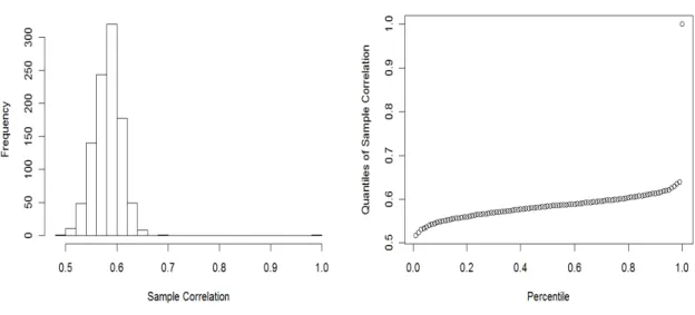
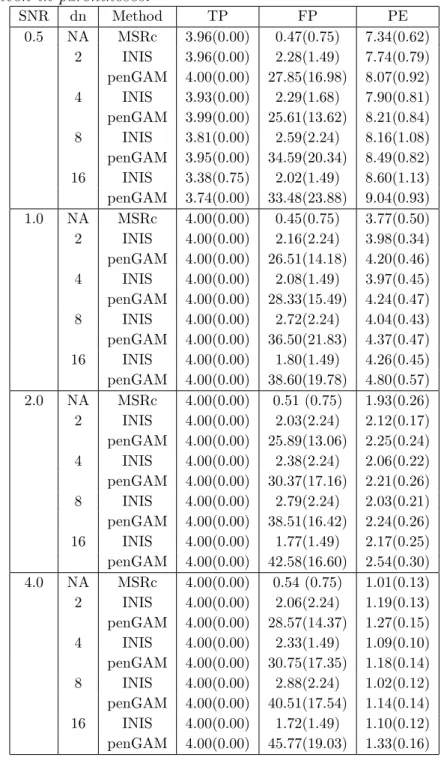
significance of the current regression estimate of the response. . . 36 3.4 Sample Correlation between X4 and Xj. Almost all correlations are smaller

(11)

List of Tables

3.1 Mean True Positive Rate and Mean False Positive Rate for Example 2. There are 100 simulations each of size 400, from which the mean true positive rate (TP) and mean false positive rate (FP) were computed. The prediction errors were computed from an independent test data of size 200 for each simulation. The mean prediction error (PE) was computed from the results of 100 simu-lations. Robust standard deviations are given in parentheses. . . 37 3.2 Mean True Positive Rate and Mean False Positive Rate for Example 3 from

100 runs. There are 100 simulations each of size 400, from which the mean true positive rate (TP) and mean false positive rate (FP) were computed. The prediction errors were computed from an independent test data of size 200 for each simulation. The mean prediction error (PE) was computed from the results of 100 runs. Robust standard deviations are given in parentheses. 38 3.3 Mean True Positive Rate and Mean False Positive Rate for Example 4. There

are 100 simulations each of size 400, from which the mean true positive rate (TP) and mean false positive rate (FP) were computed. The prediction errors were computed from an independent test data of size 200 for each simulation. The mean prediction error (PE) was computed from the results of 100 simu-lations. Robust standard deviations are given in parentheses. . . 39

(12)

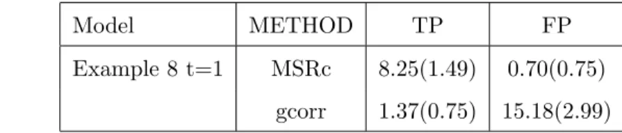
3.4 Mean True Positive Rate and Mean False Positive Rate under Different SNR in Example 5 with t=0. There are 100 simulations, each of size 400, from which the mean true positive rate (TP) and mean false positive rate (FP) were computed. The prediction errors were computed from an independent test data of size 200 for each simulation. The mean prediction error (PE) was computed from the results of 100 simulations. Robust standard deviations are given in parentheses. . . 41 3.5 Mean True Positive Rate and Mean False Positive Rate under Different SNR

in Example 5 with t=1. There are 100 simulations each of size 400, from which the mean true positive rate (TP) and mean false positive rate (FP) were computed. The prediction errors were computed from an independent test data of size 200 for each simulation. The mean prediction error (PE) was computed from the results of 100 simulations. Robust standard deviations are given in parentheses. . . 42 3.6 Comparison of MSRc and gcorr: Mean True Positive Rate and Mean False

Positive Rate. There are 100 simulations each of size 400, from which the mean true positive rate (TP) and mean false positive rate (FP) were com-puted. Robust standard deviations are given in parentheses. . . 44 3.7 Comparison of MSRc and gcorr: Mean True Positive Rate and Mean False

Positive Rate . There are 100 simulations each of size 400, from which the mean true positive rate (TP) and mean false positive rate (FP) were com-puted. Robust standard deviations are given in parentheses. . . 45 3.8 Predictive Mean Squared Errors (PMSE) on the Testing Set. Wheat data

was partitioned randomly into a training set (480 lines) and a test set (119 lines). This partitioning was repeated 50 times. PMSE for SVR models and Bayesian LASSO are fromLong et al. (2011) . . . 46

(13)

4.1 Performance Measures for Example 1. Withp= 1000, sample sizes of 60, 100, 200, and 300 were simulated 100 times, from which the mean true positive rate (TP), mean false positive rate (FP) and mean accuracy were computed. These performance measures were obtained via 3-fold CV. Robust standard deviations are given in parentheses. . . 58 4.2 Performance Measures for Example 2. Withp= 1000, sample sizes of 60, 100,

200, and 300 were simulated 100 times, from which the mean true positive rate (TP), mean false positive rate (FP) and mean accuracy were computed. These performance measures were obtained via 3-fold CV. Robust standard deviations are given in parentheses. . . 59 4.3 Performance Measures for Example 3. Withp= 1000, sample sizes of 60, 100,

200, and 300 were simulated 100 times, from which the mean true positive rate (TP), mean false positive rate (FP) and mean accuracy were computed. These performance measures were obtained via 3-fold CV. Robust standard deviations are given in parentheses. . . 61 4.4 Performance Measures with p = 12000, and n = 60,300 from simulation of

size 10. The mean true positive rate (TP), mean false positive rate (FP) and mean accuracy were computed. These performance measures were obtained via 3-fold CV. Robust standard deviations are given in parentheses. . . 62 4.5 Mean accuracy with robust standard deviations of different procedures

ob-tained from 10-fold CV with 10 runs. Performance measures for BMSF and GeneSrF are from Zhang et al.(2012). . . 65

(14)

Acknowledgments

First, I give thanks and praises to God for His marvelous work in my life during my five years of studies at Kansas State University. With that, I thank my major professor Dr. Haiyan Wang for her persistent efforts in guiding and helping me with this dissertation. My appreciation also to the committee members: Dr. Weixin Yao, Dr. Christopher Vahl, Dr. Zhijian Pei, Dr. Paul Nelson and the chair of the committee from the Math department, Dr. David Yetter. I also thank the faculty and staff of the Department of Statistics who have been very helpful throughout my studies at K-State. Thank you also to all graduate students for their friendship. Last but not the least, my sincere appreciation goes to my family members: Noel, Jaron, Mama, Papa, Manang Grace, Manung Jon, Ading Cj, Auntie Mercy and Lola for their love, encouragement and prayer support.

(15)

Chapter 1

Introduction

Given the remarkable advance in technologies and computing power, researchers are now capable of collecting very large and complex datasets. Some examples of these data are found in atmospheric science, microarrays, genomics, information technology, biogeochemical and large-scale e-commerce. In these examples, the number of covariates (p) tends to grow much faster than the number of observations (n), the so-called nonpolynomial (NP) dimensionality or ultrahigh dimensionality. The need to analyze these kinds of dataset poses a great challenge for those in the fields of statistics and machine learning. In recent years, there have been significant developments in the analysis of these datasets. But, there remains a great deal to do.

A typical problem in statistical inference is to select a parsimonious set from a large collection of covariates for the efficient prediction of the response. That is, suppose that we have a random sample (Xi, Yi),i= 1, . . . n from the population

Y =m(X) +ε (1.0.1)

in which Xi = (Xi1, . . . , Xip)T are random variables, ε is a random error with conditional

mean zero and cov(X, ε) = 0. The main objective is to estimate m(X) by minimizing the following function Σn

i=1(Yi−mb(Xi))

2_{, where} b

m(Xi) is an additive function of the components

(16)

described by the following nonlinear equation:

E(Y) = e

m(X)

1 +em(X) (1.0.2)

In this case, the main objective is to estimate m(X) such that the classification error is minimized, where m_b(X) is an additive function of the components of the argument.

Dimension reduction plays a vital role in NP or ultrahigh dimensional problems with the consideration of the sparsity assumption, which assumes that among the large number of independent variables, only a small set is related to the response variable. There exist numerous statistical procedures for data reduction and these include LARS by Efron et al. (2004), SCAD by Fan and Li (2001), and Dantzig selector by Candes and Tao (2007). However, these penalized methods are difficult to apply to ultrahigh dimensional datasets due to challenges in computational expediency, statistical accuracy and algorithmic stability. Fan and Lv (2008) proposed a two-stage screening method in which they first perform dimension reduction of the model and then apply penalized methods. This screening method called Sure Independence Screening (SIS) is successful in overcoming the aforementioned challenges. A great feature of SIS is that the dimensionality of the model is allowed to grow exponentially in the sample size. In addition, SIS requires normality of the response variable and is designed specifically for linear models. Fan and Lv (2008) also extended SIS to cover cases when the regularity conditions fail, and this methodological extension is called Iterated Sure Independence Screening (ISIS).Fan et al.(2009) developed two possible variants of SIS and ISIS that have attractive theoretical properties in terms of reducing the false selection rates. However, SIS-based screening methods are based on correlation which assumes that the response variable and covariates are normally distributed, and that the relationship of the covariates with the response is linear. Thus, SIS-based procedures are said to be methodologically challenged when the covariates are not jointly normal and when the marginal or joint regression of the covariates with the response is nonlinear. Thus, procedures for variable selection in nonparametric modeling is essential.

(17)

there is usually not enough prior information that the effects of the covariates take a linear form or belong to any parametric family. Sometimes, substantial improvements are pos-sible by using a more flexible class of nonparametric models, such as the additive model

Y =Pp

j=1mj(Xj) +ε, introduced by Stone (1985). Use of an additive model substantially

improves the flexibility of the ordinary linear model and allows transformed covariates to enter into the linear model. At present, the literature on variable selection utilizing nonpara-metric additive models is limited. Many of the available procedures are extensions of LASSO such as the sparse additive models (SpAM) by Ravikumar et al.(2009) and COSSO which is developed byLin and Zhang(2006). Another procedure is the work ofHuang et al.(2010) which is an extension of adaptive LASSO to additive models. A penalty that combines spar-sity and smoothness with a fixed design was proposed byMeier et al. (2009). Unfortunately, all of these procedures are extensions of penalized pseudolikelihood approaches to additive modeling, and hence, still suffer from the aforementioned three challenges in NP dimensional settings. A most recent screening method, Nonparametric Independence Screening (NIS), was developed by Fan et al. (2011) which is a variation of SIS based on nonparametric marginal regression. Fan et al. (2011) further improved the NIS procedure by developing the iterative NIS (INIS) and greedy-INIS. NIS-based methods consider correlation learning by ranking the magnitude of marginal estimators, nonparametric marginal correlations, and the marginal residual sum of squares. That is, one marginal nonparametric regression of the response Y are fitted against each covariate Xi separately and the importance of each

covariate to the joint model is based on a measure of the goodness of fit of their marginal models. The magnitude of these marginal utilities can preserve the non-sparsity of the joint additive models under some reasonable conditions, even with converging minimum strength of signals. NIS methods are two-stage procedures and can deal with the aforementioned three challenges better than the other methods. Nevertheless, NIS-based procedures have high false selection rate when the covariates are correlated with each other. This is because NIS-based procedures assume that the active covariates are independent of the nonactive

(18)

covariates.

The procedures that have been discussed are appropriate when the response variable is continuous. Variable selection and classification in datasets with a binary response variable is also very relevant to many fields such as in bioinformatics and image recognition. In bioinformatics, ultrahigh dimensional gene expression datasets are very common. For ex-ample, scientists want to know which of these genes have strong contribution to the binary response variable which assumes two values, namely, occurrence and non-occurrence of an event. Three of the current popular methods are Generalized Linear Models with Elastic Net (GLMNET), Binary Matrix Shuffling Filter (BMSF) and Gene Selection in Random Forest (GeneSrF). The procedure GLMNET is able to do variable selection and classification simul-taneously. On the other hand, BMSF and GeneSrF conducts variable selection. The latter two procedures are combined with classification techniques such as Support Vector machine (SVM), Naive Bayes (NB), linear discriminant analysis (LDA) and quadratic discriminant analysis (QDA) to perform classification of new observations. According to literature, the aforementioned procedures have very good performance in terms of accuracy in classifying new observations. However, GLMNET, BMSF and GeneSrF have the tendency to select many variables, which indicates that they also have the tendency to select too many false positive variables.

In general, existing procedures for both continuous and binary response variables may have the problem of selecting too many false positive variables. Motivated by this concern, this paper proposes the Most Significant Regression (MSR) algorithm which can be used for variable selection and prediction. With the high false selection rates in existing procedures, MSR algorithm aims to reduce the false selection rates.

MSR algorithm relates to the Least Angle Regression (LARS) byEfron et al. (2004) but taking into consideration the possibility of nonlinear relationships between the response and the covariates. In addition, MSR, unlike the NIS-based procedures, BMSF and GeneSrF, simultaneously conducts variable selection and response estimation. As demonstrated in

(19)

Monte Carlo simulations, results of MSR when the response variable is continuous resulted in smaller false selection rates and better predictive ability than NIS-based procedures. In addition, results of MSR when the response variable is binary showed that MSR always selects fewer variables than existing procedures while maintaining comparable classification accuracy.

(20)

Chapter 2

Literature Review

In the last decade, large data sets with large numbers of variables are more and more common. This has stimulated the development of procedures that can perform variable selection and data reduction on large data sets. Specifically, reviews of variable selection procedures and prediction techniques are discussed in this chapter.

2.1

Problems of ultrahigh dimensional setting

Richard Bellman (1961) coined the term “curse of dimensionality” which in statistics, refers to the issues caused by the rapid increase in the number of covariatespgiven a fixed sample size n. Due to the curse of dimensionality, the data are very scattered and thus, it is quite difficult to achieve accurate predictions of the response. With a very large number of covariates, unnecessary predictors may be present and will add noise to the estimation of the response. Collinearity among the predictors is also likely to exist. In addition, with very large p, the computational cost in model building is very expensive.

To avoid the curse of dimensionality, several techniques have been proposed and two of these are variable selection and additive modeling. The main goal in variable selection is to select the best subset of covariates. “Best” refers to a parsimonious model that has small sum of square error, or large adjusted R2, or low prediction error and other criteria

(21)

available in literature. Selection of the best subset of covariates can improve significantly the computational cost in estimation. On the other hand, additive modeling which was introduced by Stone(1985) can significantly improve the flexibility of the variable selection procedure.

2.2

Continuous Case

2.2.1

Variable Selection for Parametric Models

In this section, procedures for variable selection in parametric models, those that assume a linear relationship between response and predictors are discussed. Initiated by Donoho and Johnstone (1994), and following the Least Absolute Shrinkage and Selection Operator (LASSO) by Tibshirani (1996), many penalized pseudo-likelihood procedures and related methods have been studied in the literature in the setting of parametric models assuming a linear or generalized linear relationship between the response and predictors. A recent advance in ultrahigh dimensional variable selection is the development of screening methods which are deemed better than the penalized procedures in terms of statistical accuracy, computational expediency and algorithmic stability. Procedures for variable selection in the parametric setting are discussed in two separate sections, namely penalized methods and screening methods.

Penalized Methods

In high dimensional statistical endeavors, the purpose of applying the penalized methods is to simultaneously select variables and estimate the regression coefficients by maximizing the following penalized likelihood function:

n−1ln(β)− p

X

j=1

(22)

whereln(β) is the assumed log-likelihood and pλ(·) is a penalty function indexed byλ≥0, a

regularization parameter. Variables with associated estimated regression coefficients equal to zero are deleted.

Fan and Li (2001) support a penalty function that produce estimators that have the following properties: sparsity, unbiasedness and continuity. Sparsity implies that the esti-mator sets small coefficients to zero, therefore reducing the complexity of the model. For the unbiasedness property, the estimator derived from the penalty function is said to be nearly unbiased when the true parameter |βj| is large. For continuity, the resulting

estima-tor is continuous in the data to increase stability in model prediction. The following are the penalized methods developed for variable selection in ultrahigh dimensional and parametric setting.

Ridge Regression,HoerlA.E. and R.W.(1970). The main task of ridge regression is to find a linear function that models the relationships between a continuous response variable and continuous covariates. In ridge regression, the goal is to minimize the residual sum of squares (RSS) subject to a constraint of the form Σ|βj|2 ≤ t. It yields an estimator for the

regression coefficients equal toβb= (XTX+λI)−1XTy. When the covariates are highly

cor-related, ridge regression is able to restrain the size of the estimated regression coefficients by including a penalty which reduces the undesirable symptoms of correlated covariates. Using this formulation, ridge regression may be seen as a penalized L2 -regression in which

pλ(|θ|) =λ|θ|2.

Bridge Regression,Frank and Friedman(1993). Bridge regression minimizes the RSS subject to a constraint Σ|βj|q ≤ t. This procedure is a penalized Lq-regression, a natural

generalization of penalizedL0-regression in which pλ(|θ|) =λ|θ|q for 0< q ≤2. This bridges

the best subset selection (penalized L0) and ridge regression (penalized L2), including the

(23)

Least absolute shrinkage and selection operator (LASSO), Tibshirani (1996) . LASSO minimizes RSS subject to a constraint Σ|βj| ≤ t. The LASSO is also known as

the penalized L1-regression in the ordinary regression setting, in which pλ(|θ|) =λ|θ|. The

selected model in LASSO fits the mean Xβ well if its bias

Bias=k(I−Pb)Xβk

is small. Pb is the projection to the linear span of the set of selected variables and I is the

n ×n identity matrix. When θ is large, the LASSO estimator has a bias approximately of size λ ≥ 0, where λ is the regularization parameter index of the penalty function. As a result, the LASSO estimator has to choose a smaller λ in order to compensate the bias problem and obtain a desired mean squared error. However, a smaller value ofλresults in a complex model. This explains why the LASSO estimator tends to have many false positive variables in the selected model.

Smoothly clipped absolute deviation (SCAD), Fan and Li (2001). It is known that the convex Lq penalty with q > 1 fails to satisfy the sparsity condition, while the

convex L1 penalty fails to satisfy the unbiasedness condition, and the concave Lq penalty

with 0 ≤ q < 1 fails to satisfy the continuity condition. With these results, none of the

Lq penalties is able to satisfy all three properties simultaneously. For this reason, Fan and

Li (2001) introduced the SCAD which satisfies the three aforementioned properties. The SCAD penalty is given as

pλ(βj) =      λ|βj| if |βj| ≤ λ −(|βj|2−2aλ|βj|+λ2 2(a−1) ) if λ <|βj| ≤ aλ (a+1)λ2 2 if |βj| > aλ

Elastic net, Zou and Hastie (2005). This variable selection method is a linear combi-nation of L1 and L2 penalties. The main idea is to solve the optimization problem given

(24)

as βb= argmin_β|y−Xβ|2, subject to (1−α)|β|₁ +α|β|2 ≤ t for some t, and α = λ2

λ1+λ2. The function (1−α)|β|1+α|β|2 is the elastic net penalty, which is a convex combination

of the LASSO and ridge penalty. When α = 1 and when α = 0, the procedure becomes ridge regression and LASSO, respectively. One characteristic of the elastic net is its ability of selecting “grouped” variables, where strongly correlated predictors tend to be in or out of the model together. Moreover, the authors claim that this procedure in real data analysis and simulation studies outperform the LASSO in terms of prediction accuracy.

Dantzig selector, Candes and Tao (2007). This procedure is also based on penalized pseudo-likelihood which is a solution to the L1 regularization problem. The idea is rather

than controlling the size of the residuals, the Dantzig selector is based on minimizing kβk1

subject to controlling the covariance vector kn−1_XT₍_y ₋_Xβ₎_k

∞ ≤ λ, where λ ≥ 0 is a regularization parameter. Dantzig selector’s consistency for estimation and model selection depend heavily on the choice of λ. Shortly after the work on the Dantzig selector, it was observed that the Dantzig selector and the LASSO share some similarities.

Nevertheless, these methods are limited in handling ultrahigh dimensional problems due to the “curse of dimensionality”. They are simultaneously challenged in terms of com-putational expediency, statistical accuracy and algorithmic stability (Fan et al. (2011)). Motivated by these concerns, Fan and Lv(2008) and Fan et al. (2009), developed a method that is based on correlation learning.

Correlation-based Marginal Methods

Sure Independence Screening (SIS), Fan and Lv (2008) and Fan et al. (2009). The main idea of SIS is to apply a two-stage procedure which involves screening out variables that have weak correlation with the response variable, and then applying lower-dimensional

(25)

techniques such as SCAD, Dantzig selector and LASSO to further reduce the number of predictors and to estimate relevant parameters. SIS satisfies the sure screening property, that is, all the important variables are selected with probability tending to one under some conditions. In the screening stage, SIS ranks the independent variables in terms of their marginal correlations with the response. A problem in this stage is its failure to look at the joint correlation of the covariates to the response. Fan and Lv (2008) noted the possibility of the following problems in the SIS procedure: First, SIS may fail to select an important predictor that is jointly correlated but marginally uncorrelated or weakly correlated with the response; and second, when high collinearity exists among the predictors, SIS may select the unimportant predictors and exclude important predictors that are weakly correlated to the response.

Iterative Sure Independence Screening (ISIS), Fan and Lv (2008). To solve the problems in sure independence screening (SIS), the authors proposed the iterative-SIS (ISIS) which is an extension of SIS. The ISIS procedure works in the following manner: First, apply SIS and denote the set of selected variables as A1 which contains k1 variables. Obtain the

residuals from regressing the response with the selectedk1 variables. In the next step, apply

SIS procedure again with the residuals as the new responses and select k2 variables from

the p−k1 variables. Denote this set asA2 . Continue the iteration until there arel disjoint

subsets A1, A2, . . . , Al whose union has a size d < n. After the variable selection, apply a

lower-dimensional techniques such as SCAD, Dantzig selector and LASSO to further reduce the number of predictors and to estimate relevant parameters. Despite of the sure screening properties of SIS-based procedures, they have methodological challenges: SIS relies on cor-relation which assumes that the response variable and covariates are normally distributed and the marginal relationship of each covariate with the response is linear. Hence, its as-sumptions are violated when the response variable is not normally distributed and when marginal or joint relationship of the predictors with the response is highly nonlinear.

(26)

Tilting method, Cho and Fryzlewicz(2012). The main task of this method is to select important variables in linear regression models. Unlike the SIS-based procedures, during variable selection, it takes into account both the marginal and joint relationship of the pre-dictors with the response variable. To compute the correlation between a predictor,Xj and

the response,Xj is first tilted. Tilting refers to transformingXj by projecting it on the space

orthogonal to the other predictors. This approach reduces the effect of other predictors on the tilted correlation of Xj and response Y.

When the joint distribution of the response variable and covariates does not follow a normal distribution, parametric methods based on conventional correlation may not be able to detect the true relationship between the response and the covariates and therefore, may lead to incorrect selection of covariates. In addition, the presence of nonlinear marginal or nonlinear joint relationship of the covariates with the response variable results in modeling biases in the linear model. To address these issues, there is a need for nonparametric variable selection procedures.

2.2.2

Variable Selection for Nonparametric Models

Nonparametric variable selection procedures can greatly improve model building and re-sponse estimation when parametric methods are not appropriate for the data. Fan et al. (2011) in their article said that using a nonparametric modeling procedure such as the ad-ditive model by Stone(1985) can significantly improve the flexibility of the ordinary linear model and allows transformed predictors to enter into the linear model. The additive model is given as Y = Pp

j=1mj(Xj) +ε. In this section, the limited number of procedures for

(27)

Penalized Methods

Penalized methods are popular approaches in variable selection and response estimation. The following are the currently available penalized methods for the nonparametric setting.

Extensions of LASSO. Lin and Zhang (2006) proposed a penalized procedure called Component Selection and Smoothing Operator (COSSO). This procedure is a functional generalization of LASSO using the Sobolev norm penalty, and it is able to carry out model selection on either additive or non-additive models. Another method is the penalized method for additive model (penGAM) by Meier et al. (2009). In this method, the authors combine the empirical L2-norm and the usual roughness norm to enforce both sparsity and

smooth-ness. The penGAM algorithm was built on the idea of a group LASSO problem. Ravikumar et al. (2009) also proposed Sparse additive models (SpAM) which is another generalization of the LASSO that uses the empirical L2-norm of each additive component function. The

method developed byHuang et al. (2010) is also an extension of LASSO to additive models.

Multiple Kernel Learning, Koltchinskii and Yuan (2010). This procedure is devel-oped by combining empirical L2-norms and kernel Hilbert space (RKHS norms). L2 norms

are used to impose sparsity of the final model while RKHS norms are to impose the smooth-ness of the components of the additive model.

Correlation-based Methods

The penalized methods applied to additive modeling are all challenged in terms of statisti-cal accuracy, algorithmic stability and computational speed. Motivated by these concerns, methods based on correlation learning are developed.

(28)

The gcorr procedure is based on marginal screening procedure in which the generalized em-pirical correlations between the response and covariates are ranked. The authority of the ranks are assessed using bootstrap methods. The main goal of this procedure is to reduce the number of variables, after which other low-dimensional techniques such as LASSO may be applied for the prediction of the response. The gcorr procedure recruits a variable based on its marginal generalized correlation with the response Y and therefore, it ignores the collinearity that may exist among the independent variables. For this reason, gcorr leads to high false selection rate when the covariates are highly correlated.

Nonparametric Independence Screening (NIS) and its extensions, Fan et al. (2011). Nonparametric independence screening (NIS) is a nonparametric version of the sure independence screening (SIS). This procedure ranks the magnitude of marginal estimators, nonparametric marginal correlations and the marginal residual sum of squares. Specifically, the procedure fits the marginal regressions of each of the covariates with the response by employing a B-spline bases and then ranks their importance to the joint model based on the magnitude of the correlation of the marginal nonparametric estimate with the response. To select a set of variables, a threshold value is predefined. Aside from the marginal correlation, another equivalent approach of evaluating the importance of each covariate is by ranking the residual sum of squares of the componentwise nonparametric regressions. The authors extended the NIS procedure such as iterative NIS (INIS) and greedy-INIS, to reduce the false positive rate and stabilize the computation. After applying a NIS-based procedure for variable selection, a lower-dimensional technique is still required to further reduce the num-ber of predictors and to estimate relevant parameters. NIS-based procedures have the sure screening property. However, NIS-based procedures rely greatly on marginal correlations and therefore, have high false selection rates when the covariates are highly correlated.

(29)

2.2.3

Generalized Additive Models, Continuous Case

Due to the curse of dimensionality for ultrahigh dimensional problems, many nonparamet-ric methods fail to perform well. To avoid this problem, additive models was proposed by Stone (1985) which estimates the response Y using an additive approximation. Hastie and Tibshirani (1990) developed the generalized additive models (GAM) by extending additive models to a wide range of distribution families. GAM uses three techniques, namely, non-parametric regression, smoothing techniques and generalized distributional modeling. It can be applied when the relationship between the covariate and response is nonlinear, and when the distribution of the response variable belongs to the exponential family. The generalized additive model is defined as

Y =α+

p

X

i=1

hi(Xi) +,

where {Xi}’s and are orthogonal, E() = 0 and V ar() = σ2. The function hi’s are

smooth functions which are estimated in a nonparametric fashion. For univariate smoothing components, GAM procedure applies the B-spline and local regression methods, and the thin-plate smoothing spline for bivariate smoothing components. GAM uses the generalized cross validation (GCV) function as a criterion in choosing the smoothing parameters. The GCV function approximates the expected prediction error, and selects the model that has the smallest prediction error. As an alternative to using the GCV function, GAM also provides the option of specifying the degrees of freedom for each individual smoothing component.

2.3

Binary Case

2.3.1

Classification Techniques

Supervised learning with a qualitative response is considered as a classification problem. A classification problem can be further categorized into either binary classification or multi-class multi-classification. The focus of this dissertation is binary multi-classification. Classification is

(30)

a technique that is used in many fields such as in bioinformatics, document classification and image recognition. One important area in bioinformatics is disease classification given ultrahigh dimensional datasets such as gene expressions and microarrays. Classification techniques have the goal to determine a function that can be used to predict the class in which a subject belongs given the independent variables or features. When the number of independent variables is much larger than the sample size, complications occur in most of classification procedures. Among the popular classification methods include logistic regres-sion, Fisher’s Discriminant analysis (FDA), support vector machines (SVM) and k-nearest neighbor classifier.

The response variable Yi in classification problems is qualitative. It can assume two

val-ues for binary case or more than two valval-ues for the multiclass case. For example, in cancer classification, each of the covariatesXi represents the gene expression level of a patient and

Yi indicates whether this patient has cancer or not. Given a new observation X,

classifica-tion techniques aim to predict the unknown class label Y of this new observation. In this section, various classification techniques are discussed.

Classical Methods. Many classical methods were developed that can be used for clas-sification. Among the classical methods are Fisher’s linear discriminant analysis (LDA), quadratic discriminant analysis (QDA), and logistic regression. Bickel and Levina (2004) conducted a study to evaluate the performance of LDA in ultrahigh dimensional setting. In their results, LDA performs asymptotically no better than random guessing when the dimensionality p is much larger than the sample size n. For datasets with low dimension, the aforementioned classical methods perform very well. However, these methods fail when the number of covariates is much larger than the number of observations.

Distance-based classifiers. Various distance-based classifiers have been developed to deal with classification problems in ultrahigh dimensional setting. They tend to reduce

(31)

the problems arising from the curse of dimensionality. Among the list of distance-based classifiers are naive-Bayes classifier, centroid rule, and k nearest neighbor rule.

The Bayes classifier conducts classification based on the posterior probabilities of the response. It is based on Bayes theorem and uses the following equation

P(Y =k|X =x) = P(X =x|Y =k)πk

PK

i=1P(X =x|Y =i)πi

. (2.3.1)

The denominator of the equation does not need to be estimated even though it is unknown because it assumes a constant value. However, Bayes classifier breaks down in high di-mensional settings due to curse of didi-mensionality and noise accumulation when estimating

P(X|Y). The naive-Bayes classifier overcomes this problem by assuming conditional in-dependence which dramatically decreases the number of parameters to be estimated when modeling P(X|Y). Specifically, the naive Bayes classifier uses the following equation:

P(X =x|Y =k) =

p

Y

j=1

P(Xj =xj|Y =k) (2.3.2)

where Xj and xj are the jth components of X and x, respectively (see Fan et al.(2009) and

the references therein). Hence, the conditional joint distribution of the pcovariates depends only on marginal distributions. With this, naive-Bayes classifier is able to solve the problem of the curse of dimensionality. However, it assumes that the covariates are conditionally independent from each other even though they are not.

Another distance-based classifier is centroid classifier. It is a classification procedure which assigns a new observation to a class if its centroid is closest to the observation. The centroid could be the mean or median of data in class k. An extended version of centroid classifier has found applications in the medical domain, specifically classification of tumors (Tibshirani et al. (2002)).

The nearest neighbor classifier is another distance-based classifier which classifies new observations based on their similarity with observations in the training set. Given a new ob-servation, the procedure finds the k closest observations in the training data set and assigns to the class that appears most frequently within the k-subset. To determine the k closest

(32)

observations in the training data set, Euclidean distance is usually used. Larger k values may reduce the effects of noisy points within the training data set, and selecting the value for k is often done via cross-validation (Hall et al.(2005)).

Prediction Analysis for Microarrays (PAM). This approach was developed by Tib-shirani et al.(2002) intended for cancer class prediction from gene expression profiling. This method is based on an improved version of the simple nearest centroid classier. Briefly, the method classifies a new observation based on shrunken standardized centroid for each class. Standardized centroid as explained by Tibshirani et al.(2002) in their paper is the average gene expression for each gene in each class divided by the within-class standard deviation for that gene. Nearest centroid classifiers obtains gene expression profile of a new observa-tion, and compares it to the centroids of each class. The class with the nearest centroid, in squared distance, is the predicted class for that new observation. PAM uses the nearest shrunken centroid classifier in which each of the class centroids are shrunken toward the overall centroid for all classes by an amount called threshold. This shrinkage moves the centroid towards zero by threshold, setting it equal to zero if it hits zero. Nearest centroid classifier is then implemented to the shrunken class centroids. This shrinkage procedure in PAM has two advantages. First, it makes the classifier more accurate by reducing the effect of noisy genes; and second, it does automatic gene selection, that is, when a gene is shrunken to zero for all classes, then it is removed from the prediction rule. In addition, a special case of PAM sets a gene to zero for all classes except one, and high or low expression for that gene characterizes which class the new observations belong. To select the value for threshold, PAM does K-fold cross-validation for a range of threshold values. Typically, the threshold value chosen is the one which gives the minimum cross-validated misclassification error rate. Tibshirani et al. (2002) demonstrated PAM’s effectiveness in finding genes for classifying small round blue cell tumors and leukemias.

(33)

Support Vector Machines (SVM). A support vector machine (SVM) was developed with the intention to classify new observations into two classes (Cortes and Vapnik(1995)). However, SVM may also be applied to multi-class problems by treating each single class as a separate problem. Given a training data, each marked as belonging to one of two categories, a model is obtained from SVM training algorithm. An SVM model is a representation of the observations in space, mapped so that the observations of the separate classes are divided by a hyperplane that is as wide as possible. The best hyperplane is the one that represents the largest separation between the two classes. New observations are then mapped into that same space and predicted to belong to a class based on which side of the hyperplane they lie on. SVM can perform both linear and nonlinear classification. Support vector machines are usually used in bioinformatics, image recognition and text categorization. It is shown in Dumais et al. (1998) that SVM outperforms other popular methods in text categorization, such as naive Bayes and decision trees in terms of prediction accuracy and computation time.

Chang and Lin (2011) have been actively developing a library for Support Vector Ma-chines (LIBSVM). For classification, they developed c-Support Vector Classification (C-SVC) and v-Support Vector Classification (V-(C-SVC). Given training variables XiRn, i =

1, ..., lin two classes and a response binary variableY, (C-SVC) solves the following problem:

minα 1 2α T Qα−eTα subject to yTα= 0, 0≤αi ≤C, i= 1, ..., l (2.3.3)

where e = [1, ...,1]T, Q is an l × l positive definite matrix, Qij ≡ yiyjK(xi, xj), and

K(xi, xj) ≡ φ(xi)Tφ(xj) is the kernel function. On the other hand, V-SVC introduces a

new parameter ν(0,1] and the problem it solves is given as

minα 1 2α T_Qα subject to 0≤αi ≤1/l, i= 1, ..., l, eTα≥ν, yTα= 0 (2.3.4)

(34)

where Qij ≡yiyjK(xi, xj).

Classification Tree Based Methods. Decision tree methods according toRokach and Maimon (2008) are commonly used in data mining. The main goal is to build a model that predicts the value of a response variable based on several independent variables. Tree based classification methods was first introduced by Breiman et al.(1984). Three of the popular tree based procedures are bagging, random forest and boosted trees. Bagging decision trees as discussed by Breiman (1996) builds numerous decision trees by conducting a multiple resampling of training data with replacement and classification of a new observation is based on majority vote among the trees.

On the other hand, random forest was introduced independently byHo(1995) andAmit and Geman (1997). It is a combination of “bagging method” and random selection of features. To construct a model using random forest requires making choices for the shape of the decision to use for every node, the type of predictor to use for every leaf, the splitting objective to optimize for every node and the method for implementing randomness into the trees. For classification, the new observation is entered to the tree and is assigned to a class corresponding to the node where it ends up. This procedure is iterated over all trees and the observation is classified based on the majority vote of the trees.

Another tree-based method is “boosting” which iteratively grows classification trees in a sequence of reweighted datasets (Austin and Lee(2011)). In a given iteration, subjects who were misclassified in the previous iteration are given higher weights than those who were correctly classified. The final classification is based on the majority vote of classification trees.

2.3.2

Variable Selection Techniques

Variable selection is a procedure to determine the covariates that have strong contribution to the response variable. It is very important to conduct variable selection in ultrahigh

(35)

dimensional setting to avoid the curse of dimensionality. Most classification techniques fail when the number of covariates is much larger than the number of observations. Hence, for efficient classification of qualitative response variables, it is necessary to first reduce the number of covariates before implementation of classification procedures. Majority of the variable selection procedures were already discussed in Sections 2.2 and 2.3. These procedures can also be used for variable selection when the response variable is binary. In addition to these procedures, this section presents the popular variable selection procedures that are specifically used for variable selection when the response variable is binary, namely, Shrinkage methods, SVM, GLMNET, Gene Selection with Random Forest (GeneSrF) and Binary Matrix Shuffling Filter (BMSF).

Shrinkage methods. The shrinkage methods were developed for regression problems with the objective of shrinking the coefficients of some variables by imposing a penalty on their size. Among the shrinkage methods are Ridge regression and LASSO which were already discussed in Section 2.2.

Variable Selection in SVM.Guyon et al.(2002) developed a variable selection proce-dure called RFE-SVM which stands for recursive feature elimination using binary support vector machine. This procedure ranks genes using the coefficient magnitude trained from the SVM instead of ranking genes using correlation between gene and phenotype. It recursively removed covariates with smallest coefficient magnitude in the learned SVM model followed by recursively training the updated data with decreasing number of variables to re-rank the rest of genes. The authors demonstrated that the RFE-SVM has the ability to eliminate gene redundancy automatically and yielded better and more compact gene subsets. More-over,Fan and Li(2001) also developed SCAD-SVM. Both RFE-SVM and SCAD-SVM were developed using binary SVM.

Variable Selection in Random Forest. A very popular random forest procedure that can be used for binary variable selection is the Gene Selection in Random Forest (GeneSrF) which was developed byDiaz-Uriarte and Alvarez de Andres(2006) to select relevant genes

(36)

to be used for classification in gene expression studies. Its main goal is to identify the smallest possible number of genes and still result in good predictive performance. The authors have demonstrated the performance of GeneSrF through simulated and microarray data sets. In their results, random forest has comparable predictive performance to other classification methods, including KNN and SVM. In addition, GeneSrF in most data sets have yielded smaller sets of genes than alternative methods while preserving predictive accuracy.

Binary Matrix Shuffling Filter (BMSF). Zhang et al.(2012) developed the Binary Matrix Shuffling Filter (BMSF) for variable selection. This method takes into account possible gene interactions during gene selection. To perform filtering, BMSF utilizes Support Vector Machine (SVM) and eliminate variables through evaluating the effect of random sets of genes. During the gene selection process, the set of genes kept in the model was repeatedly refined and updated while taking into account the effect of a given gene on the contributions of other genes to their importance in cancer classification. Through real data sets, the authors have shown that BMSF often selects very small number of genes while preserving predictive accuracy. The significance of using BMSF includes: (1) It accounts for possible gene interactions, (2) It often selects small number of genes while accurately classify new observations, (3) It results in improved LOOCV classification accuracy when coupled with SVM, Naive Bayes (NB), linear discriminant analysis (LDA) and quadratic discriminant analysis (QDA). Results fromZhang et al.(2012) suggests that accounting for interactions among features in the search space coupled with a manageable search scheme as in BMSF provides better accuracy for biomarker selection.

Generalized Linear Models with Elastic Net (GLMNET). This procedure was developed by Jerome Friedman, Trevor Hastie and Rob Tibshirani which contains very efficient procedures for fitting elastic-net regularization paths for generalized linear models. The elastic net penalty includes mixture of ridge and lasso penalties. The GLMNET function can fit Gaussian and multiresponse Gaussian models, logistic regression, poisson regression, multinomial and grouped multinomial models and the Cox proportional hazard model. The

(37)

efficiency of the GLMNET algorithm comes from using cyclical coordinate descent in the optimization process and from underlying Fortran code. The coordinate descent update has the form e βj ← S(_N1 PN i=1wixij(yi−ye (j) i ), λα) PN i=1wix 2 ij +λ(1−α) (2.3.5)

wherey_e(_ij) =βe0+P_l6=jxilβel pertains to the fitted value excluding the contribution fromxij.

The S(z, τ) is the soft thresholding operator defined as

sign(z)(|z| −τ)+ =      z−τ if z >0 and τ <|z| z+τ if z <0 and τ <|z| 0 if τ ≥ |z|

For detailed discussion of GLMNET, please refer to Friedman et al. (2009).

2.3.3

Generalized Additive Model (GAM), Binary Case

Wood(2008) discussed the generalized additive model when the response variable is binary, that is when the outcome yi is either 0 or 1. The value 1 indicates an event and 0 indicates

no event. The objective for GAM-binary case is to model p(y|X) which is defined as the probability of an event given X = (x1, x2, ...xp)T. The generalized additive logistic model

assumes that logit(p(Y = 1|X)) =log p(y|X) 1−p(y|X) =f0 + p X j=1 fj(xij) =η(x) (2.3.7)

where the fj’s, j = 1, ..., p are smooth functions obtained via thin-plate smoothing. The

probability of an event given X = (x1, x2, ...xp)T is

p(Y = 1|X) = e (f0+Ppj=1fj(xij)) 1 +e(f0+Ppj=1fj(xij)) = e (bη) 1 +e(bη) . (2.3.8)

(38)

GAM uses the generalized cross validation (GCV) function as a criterion in choosing the smoothing parameters. The GCV function approximates the expected prediction error, and selects the model that has the smallest prediction error. As an alternative to using the GCV function, GAM also provides the option of specifying the degrees of freedom for each individual smoothing component.

(39)

Chapter 3

Continuous Case: Variable Selection

and Prediction

3.1

Introduction

In ultrahigh dimensional settings, high collinearity among the covariates is likely to exist, which makes marginal correlation screening unreliable as a measure of association between the variables and the response. Specifically, the existing nonparametric procedures are chal-lenged by the following problems (Fan and Lv(2008)):

1. Unimportant covariates are likely to enter the final model when they are highly correlated with important covariates.

2. Important covariates that are marginally uncorrelated but jointly correlated with the response are unlikely to enter the final model.

3. There exists a problem of collinearity among the covariates.

Given these problems, nonparametric marginal screening procedures such as the NIS-based procedures have high false selection rates in the final model. Hence, this paper proposes the Most Significant Regression - Continuous (MSRc) algorithm which is a variable selection and response estimation procedure that takes into account the correlation structure

(40)

among the covariates. The algorithm is a combination of smoothing spline estimation, additive modeling and tests of generalized conditional correlation procedures. It can be used with continuous or discrete response variables, and when the predictors are linearly or nonlinearly related to the response.

Comparisons with other methods such as NIS, INIS, greedy-INIS and generalized corre-lation (gcorr) are presented using the results from Monte Carlo simucorre-lations. Using a real data from genome wide association studies (GWAS), the prediction accuracy of MSRc is also compared with Support Vector Regression (SVR) Models and Bayesian LASSO which are established feature selection procedures in GWAS.

3.2

GAM in the Continuous Case

Generalized Additive Modeling (GAM) technique by Wood (2008) is implemented in the MSRc algorithm and therefore it is important to present how it was used. GAM is used to assess the significance of a smoothing spline estimate of X, say f(x), in predicting the response, say Y. The notation used in this paper isGAM(Y, f(x)). Given the variables Y

and X, GAM derives the smoothing spline estimate f(x) that minimizes the function

n X i=1 (yi−f(xi))2+λ Z ∞ −∞ [f00(x)]2dx.

The term R_−∞∞ f00(x)2_dx _{measures how wiggly} _f₍_x_{) is and} _λ _≥ _{0 is how much} _f₍_x_{) is}

penalized for being wiggly. In this paper, a thin plate regression spline basis was used and the value ofλwas selected to yield an effective degrees of freedom which is controlled by the degree of penalization selected during fitting by generalized cross validation (GCV) criterion given as

nD/(n−DoF)2,

where D refers to deviance of the model computed as D = Pn

i=1(yi −fb(xi)) 2_{, and}

b

f(xi)

is the estimate from fitting to all the data. DoF is the effective degrees of freedom of the model and n is the number of observations (Wood (2008)).

(41)

3.3

Most-Significant-Regression Algorithm, MSRc

Suppose that we have a random sample (Xi, Yi), i = 1,2, ..., n observed from an unknown

population, where Xi = (Xi1, . . . , Xip)T. We consider the case that p >> n. Suppose

that only a small subset of covariates of size p0 contribute to the response and p0 < p. For convenience of notation, we denote these p0 covariates asZi = (Xij1, . . . , Xijp0)

T_{. Moreover,}

let the true model be

Yi =m(Zi) +εi (3.3.1)

in whichYi is continuous and εi is the random error with conditional mean equal to 0. The

covariates in Zi are called active variables which we want to identify from the entire set of

covariates Ω = {Xi1, . . . , Xip}. Let X∗ = {X1∗, ..., Xm∗} be the set of variables selected to

enter the model. Initialize X∗ =φ.

Step 1: Let k= 1 , ε0(X∗) =Y, and bg = 0. The bg stores the fitted values.

Step 2: Select the first variable marginally as follows. Calculate p-values of testGAM(ε0(X∗),fb(X_j)),

for j = 1, . . . , p, where fb(X_j) is a smoothing spline estimate of ε₀(X∗), j = 1, . . . p. The

p-values are obtained for testing individual smooth terms for equality to the zero function. Choose the variable in Ω that has the smallest significant p-value (pvalue< α = 0.01) and denote it as X_k∗. If X_k∗ does not exist, terminate the algorithm. Otherwise, proceed to Step3.

Step 3: Fit εk−1(X∗) with the smoothing spline estimate of Xk∗, fb(X_k∗). Update X∗ ⇐

X∗S

{X_k∗} and Xnew ⇐Ω−X∗.

Step 4: Update _bg ⇐_bg+fb(X_k∗) and compute ε_k(X∗) =Y − b

g. If Xnew =φ, terminate the

algorithm.

Step 5: Calculate p-value of test GAM(Y,_bg). Denote it as pc.

Step 6: Calculate p-values of test GAM(εk(X∗),fb(X_j)) for all X_j X_new. If there is no

(42)

Other-wise, proceed to the next step.

Step 7: Setk =k+ 1. Select the independent variable whose p-value is close enough to pc,

that is, |pvalue−pc|<0.0005 and denote the variable as Xk∗. Then return to Step3.

The algorithm uses |pvalue−pc| < 0.0005 as a criterion for recruiting an independent

variable. The effects of this criterion are different for two scenarios.

1. If the first variable is good, that is, pc is small (close to zero), then the selection ensures

that the next variable recruited is highly significant.

2. The first variable recruited may be a false positive when active variables are marginally uncorrelated with Y, or if inactive variables are highly correlated with some active vari-ables. When the first variable recruited is a false positive, then the algorithm controls the contribution of the next variable being selected (which may also be a false positive) to be no more than the first variable in the model. The contribution is in terms of generalized correlation to be explained below.

In the algorithm, p-values from GAM(ε(X∗),fb(X_j)) for all X_j X_new test the

signif-icance of the generalized correlation between the current residual ε(X∗) and each of the smoothed function of the remaining Xj ∈ Xnew. Since the residuals are calculated based

on the variables that are already in the model, this correlation is actually the conditional generalized correlation between Y and Xj ∈ Xnew conditional on the variables selected in

earlier steps. The generalized correlation of ε(X∗) and f(Xj) is given and estimated by

ϑj = supf F cov(f(Xj), ε(X∗)) p var(f(Xj)) p var(ε(X∗₎₎ (3.3.2) b ϑj = supf F P i(f(Xij)−fj)(εi(X∗)−ε∗) q nP i(f(Xij)2−fj 2 ) q nP i(εi(X∗) 2 −ε∗2) (3.3.3) respectively, where fj =n−1 P if(Xij) and ε ∗ ₌_n−1P iεi(X ∗_).

(43)

3.3.1

Comparison of Greedy INIS and MSRc

Greedy-INIS ranks the utility of covariates according to a measure of goodness of fit such as the magnitude of marginal estimators, nonparametric marginal correlations, and the marginal residual sum of squares. In the variable screening, via thresholding, it selects a set of variables with size less than or equal to p0, a small positive integer. An example

of the threshold value is the qth _{quantile of the marginal correlations. There are three}

problems involved with this thresholding step of greedy-INIS. First, what is the most reliable threshold value? Does the threshold value depend on the judgment of the person who runs the analysis? Second, given thousands of independent variables, the threshold value selected may result in hundreds of variables being recruited. This will lead to achieving sure screening property such that all the positives are selected but very high false selection rates. Some threshold value may also result in very few variables selected which leads to very low false selection rates but very low true positive rates. Third, since greedy-INIS relies mainly on the threshold value, it will always select at least one variable to enter even though there are no variables important in predicting the response. In the case of highly correlated independent variables and when there is only one important variable used to generate Y, greedy-INIS is likely to select at least 1 variable. After variable screening, the next step is to select the final variables to enter the model by applying a more refined technique such as penGAM (Meier et al. (2009)) and SCAD (Fan and Li (2001)). Greedy-INIS mainly rely on these refined techniques to improve its false selection rates.

When p0 = 1, greedy-INIS and MSRc both recruit one variable at a time. The major

difference is the criteria on how they recruit the variable. As stated above, greedy-INIS selects a variable based on a fixed threshold value. On the other hand, MSRc selects the variable through two criteria. The first criterion applies to the recruitment of the first covariate, and it requires that the smoothing spline estimatefb(X₁∗) of a variableX₁∗ should

be significant (p-value< α= 0.01) in predicting the response. The second criterion specifies that Xk is recruited if the significance of its smoothing spline estimate fb(X_k) of the current

(44)

residual is comparable to the significance of the current regression estimate of the response. The threshold value in MSRc pertains to pc in Step 5 of the MSRc algorithm which is

updated every time a new variable is being added to the model. As a new variable is being added to the model, the residualsεk(X∗) also change. The p-values ofGAM(εk(X∗),fb(X_i))

for allXi Xnew explained in Steps 6 and Step 7 of the MSRc algorithm also change as the

residuals change. Hence, MSRc recruits a variable Xk based on the significance offb(X_k) in

predicting the current residual assessed relative to the contributions of the variables that are already in the model.

3.4

Performance Measures

To compare the performance of MSRc with existing nonparametric procedures, this paper uses the mean true positive rate (TP), mean false positive rate (FP) and mean squared prediction error (PE). Specifically, for variable selection properties, the following measures are computed:

T P =

Pr

i=1number of active variables recruited in the i

th _run

r ,

F P =

Pr

i=1number of inactive variables recruited in theith run

r ,

where r is the number of runs. Active variables are the independent variables used to generate the true model, while inactive variables are the independent variables not used in the true model. For predictive performance, independent testing is implemented to avoid overfitting that occurs when the variable selection, model building and testing are applied to the same data. That is, the prediction error (PE) is calculated on an independent test data set of size n/2. The PE is computed using the equation

P E = Pr i=1 Pn/2 j=1 (byij−yij) 2 n/2 r .

(45)

3.5

Graphical Presentation of the MSRc Algorithm

Here we illustrate the variable selection process of the MSRc algorithm with three examples. These examples use simulated data from models discussed in earlier articles.

Example 1. This is an example also discussed in Hall and Miller (2009). Suppose Wij,

j = 1, . . . ,6 and Xik, k = 5, . . . ,5000 are independent random variables which follow a

N(0,1) distribution, and let Yi = 2sin{π₂(Wi1 + 0.5Wi2)}+ P

j=3 5

Wij2 + 0.4eWi6 +Zi0 ,

Xi1 = 2Wi12+Zi1 ,Xi2 = 2Wi2+Zi2,Xi3 =Wi3Wi4+Zi3 , and Xi4 =Wi6+Zi4, where each

of the Zij’s are normally distributed with mean equal to 0 and standard deviation of 0.1.

The sample size is n = 500. This is a measurement error model in that the true covariates

Wij, j = 1, . . . ,6 are not directly observed.

Figure 3.1 presents MSRc algorithm for one simulation of data from Example 1. The first variable recruited is X3 which has a p-value equal to 1.69×10−38. It is significant at

α= 0.01 and it is the smallest among all p-values from each of the 5000 generated covariates. At this point, pcis set to be equal to 1.69×10−38. The second variable recruited isX4which

has p-value equal to 1.59×10−25_{. Note that the absolute difference of the current} _p

c and

p-value of X4 is less than 0.0005. After X4 is recruited, pc becomes 3.39×10−67. Next,X2

is recruited with p-value equal to 2.31×10−4_{. Again, the absolute difference of the current}

pc and p-value of X2 is less than 0.0005. After recruiting X2, the value of pc becomes

5.11×10−72_{. The variable recruited next is} _X

70 with p-value equal to 3.77×10−4. The

absolute difference of the current pc and p-value ofX70 is less than 0.0005. The current pc

is now equal to 3.36×10−79_{. The algorithm proceeds to finding the variable whose p-value}

is closest to the current pc. The p-value closest to the current pc is 2.39×10−3. However,

|2.39×10−3₋₃_.₃₆_×₁₀−79_|_{= 0.002 which is greater than 0.0005. Hence, the algorithm stops.}

Result comparison. For this example, the generalized correlation (gcorr) procedure by Hall and Miller (2009) implemented 500 bootstrap simulations with size n = 500 and used a prediction level of α= 0.02. With the lowest 99% percentile ranking plot, Hall and Miller (2009) selected 10 variables X3, X4, X3484, X3010, X2672, X1264, X3275, X307, X2787,

(46)

Figure 3.1: MSRc algorithm for Example 1. The covariates were recruited in the following

order: X3, X4, X2 and X70. The algorithm stopped when the |pvalue −pc| ≥ 0.0005.

The p-value is the significance of f(xk) in predicting the current residual, while pc is the

significance of the current regression estimate of the response.

pc pvalue X 3 1.694325e-38 NA X 4 3.386070e-67 1.589661e-25 X