Statistical approaches for resting state fMRI data analysis

for resting state fMRI data analysis

Guorong Wu

Proefschrift voorgedragen tot het behalen van de graad van Doctor in de Statistische Data-Analyse

Academiejaar 2015-2016

Promotor:

Prof. Dr. Daniele Marinazzo

Department of Data Analysis

Faculteit Psychologie en Pedagogische Wetenschappen, Universiteit Gent Henri Dunantlaan 1, B-9000 Gent

I would like to thank everyone who supported and helped me through the progress and completion of this dissertation.

I would like to express my appreciation and special thanks to my advisor, Prof. Dr. Daniele Marinazzo, for his continuous advice, guidance and support throughout my graduate studies at UGent.

I would like to thank Prof. Dr. Sebino Stramaglia, Prof. Dr. Wei Liao, Prof. Dr. Steven Laureys, Prof. Dr. Gopikrishna Deshpande, Prof. Dr. Dante R. Chialvo, Prof. Dr. Chris Baeken, and Dr. Enzo Tagliazucchi for their contributions to my research.

I would like to thank my parents, my wife, my brothers and sisters for their love and support.

I also acknowledge and thank my colleagues at the department of data-analysis and department of psychiatry and medical psychology for their support and encouragement. I would like to thank my friends Margarita Papadopoulou, Feng Lan, Roma Siugzdaite, Sanne Roels, Duprat Romain and Peng Zhou having fun together in Belgium. Special thanks to Isabelle, for everything she help me.

This doctoral dissertation investigates the methodology to explore brain dynamics from resting state fMRI data. A standard resting state fMRI study gives rise to massive amounts of noisy data with a complicated spatio-temporal correlation structure. There are two main objectives in the analysis of these noisy data: establishing the link between neural activity and the measured signal, and determining distributed brain networks that correspond to brain function. These measures can then be used as indicators of psychological, cognitive or pathological states. Each of these objectives is being approached through the application of various developed statistical methods: general linear model (GLM), functional and effective connectivity. GLM is a simple and powerful approach toward modeling the fMRI data, but its application relies on the exact timing of activity onset and duration, which is difficult to be obtained from resting state fMRI data without simultaneous electrophysiological recordings. Functional connectivity refers to the statistical dependence among the activity of different neural assemblies. Effective connectivity (EC) is a relatively new concept defined as the direct or indirect influence that one neural system exerts over another. It describes the dynamic directional interactions among brain regions. Concerning EC, several models have been proposed and validated: the direct transfer function, partial directed coherence, transfer entropy, Granger causality analysis, and dynamic causal models. All those methods can provide complementary insight on brains structure and function; most of them assume that the shape of the hemodynamic response function (HRF) is constant across all voxels and subjects. This may give rise to significant modeling errors in large parts of the brain, as the shape of the HRF may vary across both space and subjects. Apart from HRF confounding, redundancy is another issue that could mislead the connectivity estimation. When dealing with resting state fMRI datasets, we are always faced with high dimensionality and small sample size. A bivariate analysis would lead to the detection of many false positives, while a fully multivariate analysis could lead to computational problems due to the overfitting and the conceptual issues in presence of redundant variables.

We address HRF variability and redundancy in connectivity by using point process theory Page vii

and information theory. The statistical characteristics of point processes for individual fMRI voxels are analyzed, then the corresponding spontaneous neural event onsets are derived. Finally. the variable HRF is retrieved using a GLM. A statistical analysis of HRF shape is further addressed, validated and applied to specific datasets. Finally, a HRF deconvolution is performed on the fMRI BOLD signal to recover the intrinsic neural signal, and then the connectivity network is constructed and analyzed on the deconvolved BOLD signal. The resulting connectivity network is thoroughly validated using ad hoc datasets. Below, we give a brief outline of the thesis. The hemodynamic response function and brain connectivity are briefly reviewed inChapter 1. The variability of HRF and redundancy in brain connectivity modelling are proposed for resting state fMRI data. The fundamentals of the resting state BOLD HRF are validated in Chapter 2 by considering simulated data, ASL data, simultaneous EEG-fMRI recordings, and eyes open and closed dataset. In Chapter 3, we present the modifications to the shape of the HRF at rest following modulations of consciousness. A combined study of hemodynamic response and Granger causality based effective connectivity on chronic back pain is contained in Chapter 4. A formal expansion of the transfer entropy to address the redundancy naturally inherent to fMRI data is presented in Chapter 5. Then a toolbox implementing both dynamic functional and effective connectivity for tracking brain dynamics from functional MRI (DynamicBC) is described in Chapter 6. Finally we summarize the findings across

chapters and discuss implications and ideas for future research in Chapter 7.

Acknowledgements v Preface vii 1 General Introduction 1 1.1 Thesis objective . . . 1 1.2 Functional neuroimaging . . . 2 1.3 BOLD-fMRI . . . 4 1.3.1 Hemodynamic response . . . 5 1.3.2 Hemodynamic model . . . 7 1.3.3 Resting state HRF . . . 10

1.4 Brain mapping: from activation to networks . . . 10

1.4.1 Effective connectivity mapping . . . 11

1.4.2 Dynamic brain connectome . . . 13

2 Retrieving the HRF in rs-fMRI 15 2.1 Introduction . . . 15

2.2 Methodology . . . 16

2.3 Applications and Discussion . . . 18

2.3.1 Simulation . . . 18

2.3.2 Relation with cerebral blood flow . . . 19

2.3.3 Relation with EEG power . . . 20

2.3.4 HRF modulations with eyes open and closed . . . 22

2.3.5 HRF variability . . . 22

2.4 Conclusions and future work . . . 23 Page ix

3 Modulated spontaneous hemodynamic response to loss of consciousness 35

3.1 Introduction . . . 36

3.2 Materials and Methods . . . 37

3.2.1 Subjects . . . 37

3.2.2 Functional Data Acquisition . . . 37

3.2.3 Data Preprocessing . . . 38

3.2.4 Spontaneous point process event and HRF retrieval . . . 38

3.2.5 Statistical Analysis . . . 40

3.3 Results . . . 41

3.3.1 Spatial distributions of resting state HRF . . . 41

3.3.2 Group HRF differences and Conjunction . . . 41

3.4 Discussion . . . 42

3.4.1 Methodology considerations . . . 47

4 Point processes and connectivity in chronic pain 49 4.1 Introduction . . . 49

4.2 Materials and methods . . . 50

4.2.1 fMRI data acquisition and preprocessing . . . 50

4.2.2 Spontaneous point event detection and HRF Deconvolution . . . 51

4.2.3 Granger Causality mapping . . . 52

4.2.4 Statistical Analysis . . . 55

4.3 Results . . . 55

4.3.1 Spontaneous hemodynamic response . . . 55

4.3.2 Seed-based Granger causality mapping . . . 55

4.3.3 Joint probabilities of neural events . . . 56

4.4 Discussion . . . 57

5 Partial Decomposition of the Transfer Entropy 59 5.1 Introduction . . . 59

5.2 Methods . . . 60

5.2.1 Partial Conditioning . . . 60

5.2.2 Expansion of the Transfer Entropy to Identify Subgraphs . . . 61

5.3 Application to fMRI data . . . 64

5.3.1 Partial Decomposition . . . 64

5.3.2 Information Subgraphs . . . 65

6 DynamicBC 69 6.1 Introduction . . . 69

6.2 Function Module Implemented in DynamicBC . . . 71

6.2.1 Overview of usage of the toolbox . . . 71 Page x

6.2.4 ROI Set for Dynamic FC and EC . . . 74

6.3 Illustrations of Dynamic Brain Connectome . . . 75

6.3.1 Simulation . . . 75

6.3.2 fMRI Data . . . 75

6.3.3 Preprocessing . . . 76

6.3.4 Seed-to-voxel based static and dynamic FC patterns . . . 76

6.3.5 Seed-to-voxel based static and dynamic EC patterns . . . 77

6.3.6 ROI-to-ROI based static and dynamic FC networks . . . 77

6.3.7 Voxel-to-voxel based FC network evolved with absence seizures . . . 78

6.4 Discussion . . . 79 6.5 Conclusion . . . 80 7 General Discussion 89 7.1 Functional segregation . . . 89 7.2 Functional integration . . . 91 7.3 Future directions . . . 92 8 Scientific Output 95 9 Bibliography 97 10 Nederlandse samenvatting 115 Page xi

CHAPTER

1

General Introduction

1.1

Thesis objective

Neuroimaging is becoming a data-intensive science as its emphasis on collecting larger datasets and multimodal integration (Craddock et al., 2015). Thousands of brain imaging scans have been publicly shared so far. This enables us to investigate the neuroscien-tific questions that were previously inaccessible. Meanwhile, this growth is also quickly overwhelming the capacity of existing algorithms and tools to extract meaningful infor-mation from the data. Functional Magnetic Resonance Imaging (fMRI) is one of the most accumulated functional neuroimaging data. The high-dimensional fMRI data is typically characterized by a small sample size and high noise. It is an indirect and noisy measurement of brain activity, which captures the average effect of many spikes and does not resolve cortical columns, let alone individual neurons. A great statistical and computational effort is needed to infer the ground truth of neural activity from fMRI data (Lindquist, 2008). Nonetheless, fMRI has opened the door to quantitative yet non-invasive experiments on brain function (Ogawa et al., 1990). For instance, task-related fMRI enables us to identify and characterize functionally distinct areas in the human brain; resting state or task-free fMRI on the other hand shows lower signal noise ratio than task based fMRI, but has several advantages, especially for populations that can not perform behavioral or cognitive task (animals, development and clinical conditions). Additionally resting state fMRI is increasingly being recognized as a valid marker for clinical conditions and proxy for neural activations (Fox and Greicius, 2010; Lee et al., 2013b)). Most of resting-state fMRI studies focus on spontaneous low frequency fluctuations (≤0.1 Hz) in the blood oxygenation level dependent (BOLD) signal (Lee et al., 2013b). One of the most investigated topics is the functional architecture and of the brain derived from synchronous Page 1

General Introduction

1

activity between regions that are spatially distinct (van den Heuvel et al., 2008). However, there is evidence showing that high resting state BOLD synchronization is more likely to reflect tighter neurovascular connections (Tak et al., 2015), confirming the finding that the BOLD fluctuations depends on the contribution of neurovascular factors (Liu, 2013) (Figure 1.1). Hemodynamic response (HDR) is tightly linked with neurovascular coupling, as it reflects the complex interaction among cerebral blood flow, cerebral blood volume, and the venous oxygenation levels (Buxton et al., 1998). Even so, few studies consider the variance of hemodynamic response that may contribute to the correlations among these BOLD fluctuations. Without an explicit task design, retrieving hemodynamic response function (HRF) from resting state is a great challenge. One goal of this dissertation is to develop a set of state-of-the-art algorithms to retrieve HRF from resting state fMRI data. Another goal of this thesis concerns the improvement of the dynamical connectivity estimates at a fine scale in resting state fMRI data. As these data are typically characterized by high dimensionality and small sample size, bivariate analysis is the most employed approach to reconstruct functional architecture of the brain under stationary assumption. A large body research has shown that the nature of functional architecture is nonstationary (Hansen et al., 2015; Hutchison et al., 2013), and the bivariate method may mislead the inference of the information transfer when the effect of synergy and redundancy arise (Marinazzo et al., 2010, 2012; Stramagliaet al., 2014). To address these issue within the information theoretic framework, we aim to develop a simple and easily adoptable tools for analyzing dynamic brain networks. The ultimate goal is to obtain the maximum of information out of resting state fMRI data. In the rest of this chapter we will general overview the BOLD-fMRI, HRF model and brain connectivity.

1.2

Functional neuroimaging

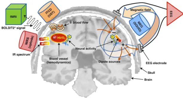
Functional neuroimaging and related neuroimaging techniques are becoming important tools for brain research. Functional neuroimaging can be used to detect or measure cognition or behavior related changes in metabolism, blood flow, etc. The aim is to understand how the brain works under different condition (pathological, cognitive, behavioral, aging). These techniques include: electroencephalography (EEG), magnetoencephalography (MEG), positron emission tomography (PET, include fludeoxyglucose for glucose metabolism, O-15 as a flow tracer, etc.), fMRI (include BOLD, perfusion, arterial spin labeling MRI, blood volume), optical imaging (near infrared spectroscopy, NIRS), functional photoacoustic microscopy, magnetic particle imaging, and transcranial magnetic stimulation (TMS), etc (Figure 1.2).

EEG and MEG have a high temporal resolution (milliseconds, accurate at recording fast changes in neural activity) but a relatively weak spatial resolution. And their source imaging is a challenge.

1

Figure 1.1: Blood supply to the human cerebrum. As illustrated here, the surface pattern of blood supply to the human cerebrum is highly complex. The red vessels are tributaries of the middle cerebral artery, the green vessels are tributaries of the anterior cerebral artery, and the blue vessels are tributaries of the posterior cerebral artery. The veins are shown in black (figure from (Huettelet al., 2004)).

Figure 1.2: Schematic diagram of brain signal detection mechanisms. EEG measures the electrical potential differences on the scalp that are generated by cortical neural activity. Neurons transmitting neurological signals across their synapses act as dipole sources. MEG detects the magnetic fields associated with such neuronal activation by SQUID sensors. fMRI measures the hemodynamic responses, particularly magnetic dynamics of protons (H+) related to neural activity; its technique is principally based on the detection of local BOLD signal contrast during neuronal activation. Using multiple arrays of optodes, NIRS characterizes changes in the intensity of attenuated near-infrared (IR) light (owing to scattering or absorption), resulting from changes in concentration between oxyhemoglobin (HbO2) and deoxyhemoglobin (Hb) during local neural activity. (figure from (Minet al., 2010))

General Introduction

1

In contrast, PET has very low temporal resolution (tens of seconds to minutes), but reasonable structural accuracy (typically falls somewhere between that of fMRI and MEG/EEG). it directly reflects the current activity (measures the distribution of glucose or oxygen uptake in the brain by evaluating the number and timing of impact of the attached radioactive isotopes) and is able to measure blood flow, oxygen use, glucose metabolism, etc.. PET scans are advantageous in that a person does not have to remain as still as he or she would for the fMRI. Tiny movements can obscure and ruin fMRI data but small movements do not affect PET scans. PET scan is more controversial than the other scans because it is rather costly, and requires injection of a trace amount of radioactivity and exposure to ionizing radiation.

FMRI has low temporal (hundreds of milliseconds or seconds) but relatively high spatial resolution. FMRI has come to dominate brain-mapping research because it does not require people to undergo shots, surgery, or to ingest substances, or be exposed to radiation, etc. fMRI can also be combined and complemented with other scans such as EEG, NIRS and PET. These hybrid-imaging technologies improve both spatial and time resolution.

1.3

BOLD-fMRI

Figure 1.3: Left: summary of BOLD signal generation. Under normal conditions, oxygenated hemoglobin is converted to deoxygenated hemoglobin at a constant rate within the capillary bed (A). But when neurons become active, there is an increase in the supply of oxygenated hemoglobin above that needed by the neurons (B). This results in a relative decrease in the amount of deoxygenated hemoglobin and a corresponding decrease in the signal loss due to T2* effects. Right (C): Changes in oxygenated and deoxygenated hemoglobin following neuronal stimulation (figure from (Huettelet al., 2004)).

1

(Ogawa et al., 1990). Increases in neural activity will elicit an increase in oxygen and glucose consumption supplied by the vascular system, then cause variations in microvascular oxygenation, more precisely, the ratio between oxygenated hemoglobin (diamagnetic) and deoxyhemoglobin (dHb, paramagnetic) changed, which in turn cause magnetization changes that can be detected in an MRI scanner. This method necessarily examines the oxygenation changes in venous blood because arterial blood is essentially completely oxygenated blood (oxygenation in arteries is always 90-100%) (McIntyre et al., 2003) (Figure 1.3).

It’s worth mentioning that the BOLD signal changes caused by neuronal processes are associated with synaptic inputs at the site of activation, not with the output level of firing of the neuron receiving synaptic inputs (Logothetis et al., 2001). This means that BOLD signal reflects the synaptic activity driving neuronal assemblies, but cannot disclose the information content of the neuronal firing patterns produced by the neurons (Ogawa and Sung, 2007), and indicates the relationship between the BOLD signal and a neural excitation or inhibition is not straightforward. However, accumulated evidences suggest that synaptic activity related to excitatory (EPSP) and inhibitory (IPSP) potentials leads to observe a positive BOLD response (Logothetis, 2003; Lauritzen, 2005); but a decrease in local neural activity leads to a negative BOLD response (Shmuel et al., 2006; Pasley et al., 2007). It is also possible for the BOLD signal to change without local neural activity changes, such as due to the physiological variations in cerebral circulation (Ogawa and Sung, 2007).

The previous studies show that BOLD changes detected in fMRI experiments vary around 1 ∼ 10%. While some activation-induced signal changes will be contaminated by large surface vessel signals (reach very large value of 10 ∼20%) (Figure 1.1) (Ogawa and Sung, 2007). Apart from the local vascular structure and brain anatomy, several other factors could also directly influence the BOLD signal: instrumental factors such as the magnetic field strength; the size of the voxels, and the age of the subject etc. Task parameters can also exert an influence on the magnitude of the BOLD signal change.

1.3.1

Hemodynamic response

The change in the MRI signal from neuronal activity is typically referred to as the hemodynamic response. There are some typical characteristics in stimulus-evoked HDR: it increases about 1∼ 2 second after neuronal activity and peaks up to plateau at about 5 ∼ 8s. In some cases, an initial decrease of the BOLD is observed call the initial dip, after the end of the stimulus, a poststimulus undershoot can often been observed (Figure 1.4, Top).

Though BOLD response offers only an indirect measure of the neural activity, it provides an interesting insight to the underling neural activity. Modeling the shape of HDR thus Page 5

General Introduction

1

plays an important role in the quantification of neural activity.

Figure 1.4: Top: BOLD HRF to an event stimulus applied at time t = 0s (figure from (Francis and Panchuelo, 2014)). Bottom: Relative changes in cerebral blood flow and cerebral blood volume following neuronal activity (figure from (Huettelet al., 2004)). CBF: cerebral blood flow; CBV: cerebral blood volume.

HDR is being studied almost from the beginning of fMRI. As mentioned before, several artifacts can corrupt BOLD-fMRI data; thus, its a great challenge to accurately and robustly model the HDR. There are two different approaches in modeling the hemodynamic response function in the literature. The most common approach is purely heuristic, using known functions (e.g. Poisson and Gaussian distributions (Friston, 1994; Rajapakse et al., 1998), and gamma functions (Boynton et al., 1996)). The second approach is biophysically informed non-linear models, such as the Balloon model (Buxton et al., 1998), which Page 6

1

volume (Figure 1.4, bottom). A more detail description of HRF model will be reviewed in the follow-up section.

1.3.2

Hemodynamic model

Considering the BOLD response linearly dependent on the underling neural activity is a reasonable first approximation over restricted ranges (Boynton et al., 1996). Mapping of stimulus or task-related BOLD Changes become possible with a general linear model (GLM). Then the BOLD response to arbitrary stimulus can be predicted from stimulus/task time course and the systems impulse response function (i.e. HRF, h(t)) (Penny et al., 2011) :

X(t) =u(t)⊗h(t) = Z T

0

u(t−τ)h(τ)dτ (1.1)

Where X(t) represents the predicted BOLD response arising from neural activity; u(t) indicate the stimulus function (usually the stick function or boxcar function encoding the occurrence of an event or epoch, u(t) = PK

i=1αiδ(t−t

i_{), where δ(t) is the Dirac delta}

function); τ indexes the peristimulus time (PST), over which the BOLD impulse response is expressed.

Although the exact mechanisms underlying the HRF are not yet completely known, the HRF appears similar across early sensory regions, such as V1 (Boynton et al., 1996), A1 (Josephs et al., 1997) and S1 (Zarahn et al., 1997), these consistency of its observed shape

allowed for canonical HRF models to be derived.

Among these HRF models, double Gamma models are the most frequently employed HRF in fMRI studies, h(t) =A tα1−1_βα1 1 e−β1t Γ(α1) −ct α2−1_βα2 2 e−β2t Γ(α2) (1.2) Where A controls the amplitude, α and β control the shape and scale, respectively, and

c determines the ratio of the response to undershoot. Γ represents the gamma function, which acts as a normalizing parameter. α,β and c are fixed in canonical double Gamma HRF, which could not fully account for HRF variability and may lead to mis-modeling of the signal in large portions of the brain. However, as six parameters are involved in this model, the computation are more expensive, and optimal model fits can always result in physiologically ambiguous or implausible results, though there exist many excellent algorithms, such as Levenberg-Marquardt algorithm (Mor´e, 1978).

To accommodate the HRF variability, a simplest way to achieve this with GLM is via an Page 7

General Introduction

1

expansion in terms of m temporal basis functions, hi(t):

h(τ) =

m

X

i=1

bihi(τ) (1.3)

Then the GLM equation in 1.1 can be written:

X(t) = K X i=1 m X j=1 bjhj(t−ti) (1.4)

Where bj are the parameters to be estimated. Several temporal basis sets are employed in

fMRI studies, here only the following basis sets are introduced:

1. Canonical HRF with its partial derivatives used in SPM package, which allow for small shifts in both the onset and width of the canonical HRF. The fixed values (α, β and c) in canonical two gamma functions HRF were derived from a principal component analysis (PCA) of the data reported in (Friston et al., 1998b). For example, if the real BOLD impulse response is shifted by a small amount in time

τ, then by the first-order Taylor expansion: h(t+τ) ≈h(t) +τ h0(t). Then small changes in the latency of the response can be captured by the parameter estimate for the temporal derivative. A similar logic applies to the use of dispersion derivative to capture (small) differences in the duration of the peak response. Together, these three functions comprise SPMs informed basis. Subsequent work, using more biophysically informed models of the hemodynamic response, revealed that the informed set is almost identical to the principal components of variation, with respect to the parameters of the Balloon model described in follow-up section (Penny et al., 2011). 2. FLOBS (FMRIBs Linear Optimal Basis Set) (Woolrich et al., 2004), which allows

the specification of sensible ranges for various HRF-controlling parameters (delays and heights for the different parts of the HRF convolution kernel), generates lots of example HRFs where each timing/height parameter is randomly sampled from the range specified, and then uses PCA to generate a basis set that optimally spans the space of the generated samples.

3. With the least assumptions about the shape of response: finite impulse response (FIR) and Fouries basis sets. However, optimal designs for estimation of their parameters are much more need than canonical HRF and FLOBS (Josephs and Henson, 1999; Miezinet al., 2000; Liu, 2004; Liu and Frank, 2004). In FIR model, the BOLD response of a certain voxel at timet is the weighted sum of the stimulus values (si, i∈[t−n+ 1, t]) at the preceding n time points, i.e. yt(w) =

P

wist−(i−1)+w0.

The optimal estimate ofw= [w0, w1,· · · , wn] T

is taken to minimize the total squared error between the observations and the model. To avoid overfitting problem in Page 8

1

a maximum a posteriori parameter estimation similar to ridge regression (Goutte et al., 2000),wM AP = STS+σ2Σ−1 −1 ST_{y, where Σ} ij = υexp −h₂(i−j)2 , where

h is a smoothing factor and Goutte recommends that this value be set a priori to

h = _{T R}7 − 1

2_{, σ}2 _{is the variance of noise, and υ is the strength. Such a smoothing} induces a correlation among parameters and prevents sudden changes in the local form of the HRF. So far, there are several convenient toolkits has been developed to perform the FIR related HRF recovery (Pedregosa et al., 2015; Vincent et al., 2014).

For a critical evaluation of these basis sets (especially the canonical HRF with partial derivatives, and FIR), see (Lindquist and Wager, 2007; Lindquist et al., 2009). These approaches could capture variations in HRF, but they do not provide a biophysical foundation for the HRF model, hence limiting the physiological interpretability of the associated parameters. Moreover, they do not explain empirically observed nonlinearities in the BOLD responses (Birn et al., 2001).

Nonlinearities are believed to arise from nonlinearities both in the vascular response and at the neuronal level (Sheth et al., 2004), and are commonly expressed as interactions among stimuli (Friston et al., 2000). In the presence of significant deviation from the expected linear system behavior, the GLM is not applicable for modelling BOLD signal. Using a biophysically informed model of the HRF can more accurately explains commonly observed non-linearities, and allows for a physiologically plausible interpretation of the results (Rosa et al., 2015). Then two main types of nonlinear models for fMRI have been proposed: the Ballon model and its extensions (Buxton et al., 1998, 2004), and the Volterra series based models (Friston et al., 2000).

The Balloon model is an input-state-output model; it describes the changes in blood oxygenation, cerebral blood flow and cerebral blood volume, as a consequence of the regional increase in brain metabolism associated with neuronal activity (Buxton et al., 1998). While the Volterra series model is an extension from the GLM, is a model for nonlinear behavior similar to the Taylor series. The second-order Volterra series are the most commonly used for simplicity, but flexible enough to accommodate a variety of nonlinear hemodynamic behaviors across different regions, stimuli and subjects (Friston et al., 2000; Zhang et al., 2014a). Unfortunately, due to much higher conceptual and computational complexity and higher number of state variables and parameters to be estimated (compare to GLM methods), these models have been usually remitted to studies in which the knowledge of the physiological events is important or essential.

In this dissertation, we only review the HRF model with linear and nonlinear framework. However, according to the different classified methods, the HRF model could be classified in different ways, such as parametric and nonparametric approaches (see (Zhang et al., 2014a).for a brief review).

General Introduction

1

1.3.3

Resting state HRF

The GLM-based method is dependent on the knowledge of stimulus function. For task related fMRI, the stimulus inputs (such as sensory stimuli or cognitive tasks) could be measured; while for resting state fMRI, no explicit external inputs exist. The simultaneous recordings of electrode may help to obtain resting state neural event information, also growing evidence indicates discrete neuronal events occur when the brain at rest (Deco and Jirsa, 2012; Tagliazucchi et al., 2012a; Petridou et al., 2013; Wu et al., 2013a). The corresponding spontaneous BOLD event can be detected by point process without multimodal monitoring (Tagliazucchi et al., 2012a; Wu et al., 2013a).

The dynamic Balloon model is a state-space model. Generalized filtering (Friston et al., 2010) and cubature Kalman filtering (Havlicek et al., 2011) has been proposed for the Balloon model inversion. Moreover, the information of stimulus inputs is not required in these methods. So it is another choice for resting state HRF analysis.

1.4

Brain mapping: from activation to networks

The GLM approach is one of the most common statistical methods to localize areas of the brain that activate in response to certain task. Apart from identification of the functional network of sites participating in a functional task, it can be also used to assess functional specificity of the activated sites by the carefully chosen paradigms (such as, to estimate whether the site only responds to a single psychological event type, or several types of events).

To understand how the brain works we also need to know the functional network of sites participating in a functional task, i.e. functional integration, or brain connectivity. A number of connectivity methods have been proposed to quantify information transfer among these sites. In the neuroimaging literature, the brain connectivity has been mainly characterized by anatomical, functional and effective connectivity. Anatomical connectivity is commonly based on white matter tracts quantified by diffusion tractography (Hagmann et al., 2008); functional connectivity relies on the other hand on statistical dependencies such as temporal correlation (Salvador et al., 2005). An important addition to this framework can come from effective connectivity analysis (Friston, 2011), in which the flow of information between even remote brain regions is inferred by the parameters of a predictive dynamical model.

1

1.4.1

Effective connectivity mapping

Granger causality

For some techniques, such as dynamic causal modelling (DCM) and structural equation modelling (McLntosh and Gonzalez-Lima, 1994; Buchel and Friston, 1997; Friston et al., 2003), these models are built and validated from specific anatomical and physiological hypotheses. Other techniques such as Granger causality analysis (GCA) (Bressler and Seth, 2011), are on the other hand data-driven and rely purely on statistical prediction and temporal precedence (Figure 1.5). While powerful and widely applicable, this last approach could suffer from two main limitations when applied to BOLD- fMRI data: confounding effect of HRF and conditioning to a large number of variables in presence of short time series.

Figure 1.5: Two fMRI signals with temporal dependence.

Early interpretation of fMRI based directed connectivity by GCA always assumed ho-mogeneous hemodynamic processes over the brain; several studies have pointed out that this is indeed not the case and that we are faced with variable HRF latency across physi-ological processes and distinct brain regions (Roebroeck et al., 2011; Valdes-Sosa et al., 2011). Recently, a number of studies have addressed this issue proposing to model the HRF according to several recipes (Havlicek et al., 2010, 2011; Ryali et al., 2011; Kadkho-daeian Bakhtiari and Hossein-Zadeh, 2012). As well, a recent study has proposed that it would still feasible to infer connectivity at BOLD level, under the assumption that Granger causality is theoretically invariant under filtering (Bressler and Seth, 2011) and that the HRF can be considered as a filter. It is still unclear whether and how specific effects related to HRF disturb the inference of temporal precedence. In addition a simulated or experimental ground truth is difficult to obtain, though some studies on simulated fMRI data have tried to reveal the relationship between neural-level and BOLD-level causal influence (Deshpande et al., 2010; Deshpande and Hu, 2012; Smith et al., 2011;

General Introduction

1

Wen et al., 2013). A considerable help to obtain the HRF for deconvolution could come from multimodal imaging where the high temporal resolution of EEG is combined to the high spatial resolution of fMRI, but this experimental approach is still far from being optimal and widely applicable. HRF has been studied almost since the early days of fMRI (Handwerker et al., 2012a). For task-related fMRI, neural population dynamics can be captured by modeling signal dynamics with explicit exogenous inputs (Riera et al., 2004; Friston et al., 2008) i.e. deconvolution according to the explicit task design is possible in this case (Glover, 1999; Friston et al., 2000) . For resting-state fMRI on the other hand, the absence of explicit inputs makes this task more difficult, unless relying on some specific prior physiological hypothesis (Fristonet al., 2008; Havlicek et al., 2011). To overcome this limitation, a novel blind deconvolution technique was developed recently for resting-state BOLD-fMRI signal (Wu et al., 2013a).

Coming to the second limitation, in order to distinguish among direct and mediated influences in multivariate datasets it is necessary to condition the analysis to other variables. A bivariate analysis would indeed lead to the detection of many false positives. In presence of a large number of variable and short time series, a fully multivariate conditioning could lead to computational problems due to the overfitting. Furthermore, conceptual issues would arise in presence of redundant variables (Angelini et al., 2010; Marinazzo et al., 2010; Stramaglia et al., 2014). To cope with redundancy and dimensionality curse in evaluating multivariate GC, it has recently been proposed (Marinazzo et al., 2012) that conditioning on a small number of variables, chosen as the most informative ones for each given candidate driver, can be enough to recover a network eliminating spurious influences, in particular when the connectivity pattern is sparse.

Transfer entropy

Transfer entropy (TE) is a rigorous derivation of a Wiener-Granger causal measure within the information theoretic framework (Schreiber, 2000). More specifically, transfer entropy from a process X to another process Y is the amount of uncertainty reduced in future values of Y by knowing the past values of X given past values of Y, i.e.

T EX→Y =H(Yt|Yt−1:t−L)−H(Yt |Yt−1:t−L, Xt−1:t−L) (1.5)

Where H(X) is Shannon entropy of X.

In principle, TE does not assume any particular model for the interaction between the two variable. Thus, the sensitivity of TE to all order correlations becomes an advantage for exploratory analyses over GC or other model based approaches. This is particularly relevant when the detection of some unknown non-linear interactions is required (Vicente et al., 2011). However, it usually requires more samples for accurate estimation (Pereda et al., 2005), which is one of the major obstacles to its application in fMRI data.

1

1.4.2

Dynamic brain connectome

Though it is often stated that dynamic interactions between brain regions constitute the basis of cognition, the majority of extant functional connections MRI studies assume temporal stationarity of connectivity metrics across a given period. A large body research has shown changes in connectivity metrics over time (Hutchisonet al., 2013; Calhounet al., 2014). Thus, the assumption that FC measures are constant over time is overly simplistic, and do not provide information critical to understanding how the brain produces cognition. What is needed is not only what is connected, but how and in what directions regions of the brain are connected: what signals they convey and how those signals are acted upon as part of a neural computational process (Bargmann and Marder, 2013; Kopell et al., 2014). Simulation and empirical studies indicate that functional connectivity dynamics bear promise to serve as a better biomarker of resting state neural activity and of its pathologic alterations (Hutchison et al., 2013; Zalesky et al., 2014; Hansen et al., 2015). These evidences suggest that dynamic FC metrics may index changes in macroscopic neural activity patterns underlying critical aspects of cognition and behavior, though limitations with regard to analysis and interpretation remain (Hutchison et al., 2013).

Retrieving the Hemodynamic Response Function in resting state

fMRI: methodology and applications

Abstract

In this chapter we present a procedure to retrieve the hemodynamic response function from resting state (RS) fMRI data. The fundamentals of the procedure are further validated by a simulation and with ASL data. We then present the modifications to the shape of the HRF at rest when opening and closing the eyes using a simultaneous EEG-fMRI dataset. Finally, the HRF variability is further validated on a test-retest dataset.

2.1

Introduction

Functional MRI time series can be modeled as the convolution of a latent neural signal (which is not measured) and the hemodynamic response function (HRF). First, since the temporal characteristics of the HRF across different anatomical regions can be influenced by the underlying venous structure, it is possible that intrinsic activity across disparate brain regions can be temporally correlated owing to the underlying vascular architecture. Second, the hemodynamic response is affected by physiological fluctuations arising from cardiac pulsation and respiration (Cordes et al., 2001). These can introduce temporal correlations in fMRI signals. Also, given the fact that fMRI data is sampled slowly (typically every 1∼2 seconds), physiological fluctuations cannot be removed by simple filtering as they can alias into the low frequency band of interest (0.01∼0.1 Hz). Third, the period of the fastest variation in RS-fMRI data is 10 s, which is orders of magnitude greater than the sub-second time scale at which most neuronal processes occur. This Page 15

Retrieving the HRF in rs-fMRI

2

confounding effect can be dealt with by deconvolution of the HRF. In task-related fMRI this procedure has been known and applied since the very beginnings (Gitelman et al., 2003), since the onset of the HRF was known. This is not the case for RS-fMRI. Motivated by this evidence, we developed an approach to perform blind hemodynamic deconvolution of RS-fMRI data to recover the underlying latent neuronal signals (Wu et al., 2013a). This greatly improved the estimation of directed dynamical influences in RS-fMRI recordings , but also provided us with an estimation of the HRF shape for each voxel in the brain (Wu et al., 2013a). In this chapter we will first validate the blind HRF retrieval approach by means of a simulation and a comparison with baseline CBF, then we will analyze the effects of physiological conditions (eyes open vs. eyes closed) on the HRF shape; finally the HRF variability will be assessed with the help of a test-retest resting state fMRI dataset.

2.2

Methodology

The deconvolution is blind because there is no external input in case of RS-fMRI data and consequently, both the HRF and the underlying neuronal latent variables must be simultaneously estimated from the observed fMRI data, making this an ill-posed estimation problem.

We will now briefly review the foundations of a blind HRF retrieval technique for resting-state BOLD-fMRI signal developed in a previous work (Wu et al., 2013a). There is accumulated evidence of specific BOLD events governing the dynamics of the brain at rest (Tagliazucchi et al., 2012a; Petridou et al., 2013). We start from the assumption that resting-state brain dynamics can be driven by spontaneous events, which can be seen as a point process. A linear time invariant (LTI) system is used to model the relationship between the spontaneous neural event and the BOLD response. The hemodynamic response

h(t) represents such dynamic process; the BOLD signal at timet, y(t), is modeled as the convolution of neural state s(t) andh(t), i.e.

y(t) =s(t)⊗h(t) +(t) (2.1) where⊗ denotes convolution, and (t) is the unexplained error.

The right side of the above equation includes three unobserved quantities. In order to solve the equation for h(t) we need to substitute s(t) with a hypothetical model of the neural activation for s(t). Here we employ a stimulus function ˆs(t) to model s(t). ˆs(t) is constituted by several time-shifted delta functions, which are centered at the onset of each spontaneous point process events. For task-related fMRI, the stimulus function is always derived according to the prior task design information. This is not the case for resting state fMRI. We need to retrieve the spontaneous point process event from a given signature (spike/peak) in the BOLD time series. As the peak of the BOLD signal lags Page 16

2

BOLD spikes are generated from the spontaneous point process events.

In order to obtain the time lag κ, we search all values in the interval [0, P ST], where PST is the peristimulus time, choosing the one for which the noise squared error (i.e. |y(t)−sˆ(t)⊗h(t)|2_{) is smallest, indicating the spontaneous event onset. In practice, The}

timing set S of these resting-state BOLD spikes/transients is defined as the time points exceeding a given threshold µaround a local peak, which can be detected according to the following expression:

S{i}=ti, y(ti)≥µ&y(ti)≥y(ti−τ) &y(ti)≥y(ti+τ) (2.2) It is worth mentioning that we make no assumption about the exact shape or functional form of the hemodynamic responses. The application of prior knowledge about possible hemodynamic response shapes could reduce the bias in the linear estimation framework especially for the low signal noise ratio dataset, and sharply reduce the computational cost. Therefore, we assume that the hemodynamic responses for all resting state spontaneous point process events and at all locations in the brain are fully contained in and-dimensional linear sub-space H ofRd, then, any hemodynamic response h can be represented uniquely as the linear combination of the corresponding basis vectors. The canonical HRF with its delay and dispersion derivatives (we denote it as canon2dd) are employed as the basis functions in our previous study (Wu et al., 2013a). The HRF can also be reconstructed via (smoothed) Finite Impulse Response (sFIR) (Ciuciu et al., 2003; Lindquist and Wager, 2007) or ’selective averaging’ (Dale and Buckner, 1997). There are some implicit limitations in our previous work described so far.

1. ∼N(0, σ2_{) is assumed to be white. However, is not independent in time due to}

aliased biorhythms and intrinsic neural activity not accounted for in the model. 2. The spontaneous point process event onsets need to be synchronized with scans, i.e.

the time lag κ is an integral multiple of TR, which may induce some bias. 3. in equation 2.1, the baseline activity is not included.

To reduce the above estimation bias, we modify the algorithm to account for the temporal dependency in , and the mismatching between events onset and scans, in the following way:

1. Using an AR(p) model during the parameter estimation of temporal correlation structure in (t).

2. Estimating the time lag in a much finer temporal grid rather than TR, i.e. the peak of BOLD response lags behind the peak of neural activation is presumed to

κ×TR/N seconds (where 0≺κ≺PST ×N/TR).

Retrieving the HRF in rs-fMRI

2

3. Adding a constant term into equation 2.1,

y(t) = s(t)⊗h(t) +c+(t) (2.3) wherec indicates the baseline magnitude of the BOLD response.

To characterize the shape of the hemodynamic response, three parameters of the HRF, namely response height and its normalization (normalized by baseline magnitude c, i.e. percent signal change, PSC), time to peak, Full Width at Half Maximum (FWHM), were estimated. These quantities are interpretable in terms of potential proxies for response magnitude, latency and duration of neuronal activity (Lindquist and Wager, 2007). The procedure described above is sketched in Figure 2.1.

Figure 2.1: scheme of the resting state HRF retrieving procedure.

2.3

Applications and Discussion

2.3.1

Simulation

To validate the feasibility and effectiveness of proposed algorithm, the simulated HRFs are used as the ground truth for simulations. The HRF was generated using a physiological model, the balloon model (Buxton et al., 1998), with TR=2s and the parameters used SPM package: signal delay = 0.64, autoregulation= 0.32, exponent for Fout(v) = 0.32,

resting oxygen extraction = 0.4, and varying transit time (τ0) = 0.98, 1.3, 1.6, 2. The

transit time is V0/F0, where V0 is resting blood volume fraction andF0 is resting flow. The

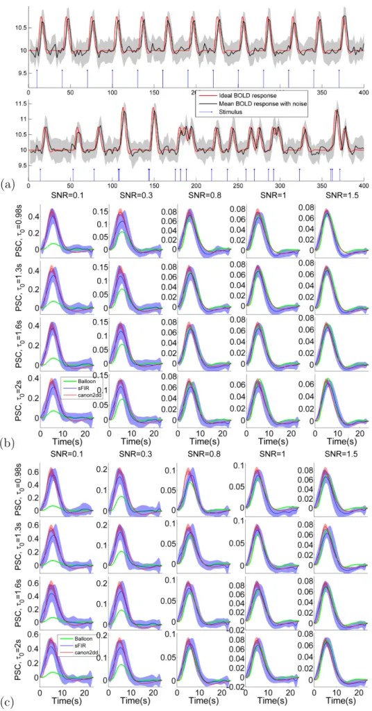
physiology of the relationship between flow and volume is determined by the evolution of the transit time (Friston et al., 2000). Two types of stimulus designs are employed to simulate the BOLD signal:

2

2. Jittered ER design with non-uniform ISI (average ISI = 19s).

Different levels of white noise , modeled by an autoregressive AR(1) process with AR coefficient of 0.2, are added such that the resulting SNR (σSignal/σN oise, where σ is the

standard deviation) are 1.5 (low noise) and 0.1 (high noise). Each ER design simulation is run 20 times with random values of in order to generate a null distribution (in order to ensure reliability of the result and compute the mean and standard deviation of the HRF). We observed that the retrieved HRF shapes are dependent on the SNR. As expected, the variability of canon2dd HRF is much lower than sFIR model across all level of SNR, both for fixed and non-uniform ISI. As shown in Figure 2.2, two HRF basis vectors show similar but different degree of fitting of ground truth HRF, slightly vary with different transit times. These stable characteristics implicate that the proposed algorithm could be a robust indicator of spontaneous BOLD response. Besides, as the balloon model is a nonlinear HRF model, the jittered design may induce nonlinear interaction between stimuli, which could violate the assumption behind the proposed algorithm (Boynton et al., 2012).

2.3.2

Relation with cerebral blood flow

The BOLD-fMRI signal reflects the complex interactions between cerebral metabolic rate of oxygen, cerebral blood flow (CBF) and volume; the comparison of CBF and HRF in the same voxels could provide a better understanding of the temporal dynamics of resting state spontaneous responses. In this section we employ a public dataset (Avants et al., 2015) to explore the relationship between baseline CBF and HRF.

The resting state BOLD fMRI images were acquired using 2D EPI sequence (TR=2s, 8 min). Subjects (N=108, some of them with longitudinal data) were required to relax quietly while looking at a fixation point. Pseudo continuous arterial spin labeled (pCASL) images were acquired using gradient-EPI with TR/TE=4,000/12ms. The total imaging time was 5.5 min, and 40 label/control pairs were acquired, with 1.5s labeling duration and 1.2s post-labeling delay.

BOLD fMRI images were preprocessed with SPM12, including: realigning and unwarping, coregistration to anatomical image, spatial normalization into MNI space, smoothing (8 mm FWHM Gaussian kernel), detrending, and linear regression to remove possible spurious variances from the data (including six head motion parameters, non-neuronal sources of noise estimated using the anatomical component correction method, i.e. white matter and cerebral spinal fluid signal), 0.008 ∼ 0.1Hz band filtering. As the slice order information is not reported in this dataset, we did not perform the slice timing correction, which does not affect the HRF retrieving algorithm anyway. pCASL data were preprocessed using the ASLtbx toolbox (Wanget al., 2008), with the following steps: realigning, coregistration to Page 19

Retrieving the HRF in rs-fMRI

2

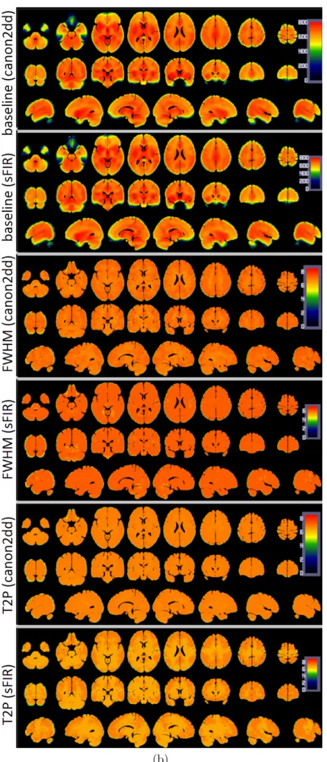
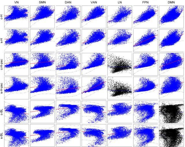
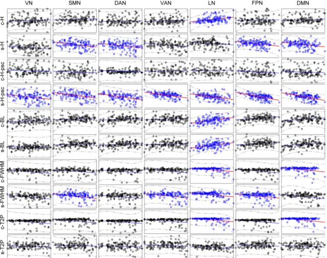
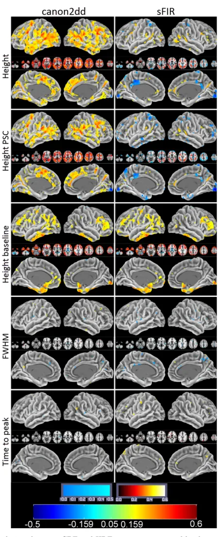
anatomical image, regression of the six head motion parameters and smoothing with 6mm FWHM Gaussian kernel. CBF was then estimated, and finally normalization to MNI space was performed (same normalization method used in BOLD fMRI images). The group median map of CBF and HRF parameters are presented in Figure 2.3. We can observe that the HRF response height shows a spatial pattern similar to the CBF map. A prior functional parcellation of cerebrum is applied to the median map to validate the effect of spatial correlations between them. The prior functional parcellation is composed of seven large-scale subnetworks: visual (VN), somatomotor (SMN), dorsal attention (DAN), ventral attention (VAN), limbic (LN), frontoparietal (FPN) and default network (DMN) (Yeo et al., 2011). The correlation analysis across voxels in each subnetworks showed a striking spatial overlap between CBF and HRF response height (PSC, baseline) (Figure 2.4). Such phenomenon is not observed in other HRF parameters. In particular there is evidence of a highly nonlinear relationship between height PSC/baseline and CBF. In the DMN (baseline) and LN (height PSC), the linear relation is not evident, both for canon2dd and sFIR model. Furthermore, the across subject correlation between CBF and HRF were also analyzed both at voxel level and large-scale network level (Figure 2.5, 2.6). We found that different HRF models show different correlation with CBF at both spatial resolutions. In contrast to canon2dd, sFIR shows higher correlation in HRF response height, lower in time to peak. The physiological basis of this complicated interaction will need to be investigated further.

2.3.3

Relation with EEG power

In order to further investigate the electrophysiological basis of the HRF and its coupling to electrical brain activity we considered simultaneously recorded EEG and fMRI data. EEG were collected at 1000 Hz and down-sampled at 250 Hz. Scanner artifact correction, pulse artifact correction, notch filtering and ICA analysis were performed on the raw data. fMRI data were collected at 7 Tesla, with a repetition time of 1s. Resting-state fMRI data preprocessing was carried out using both AFNI and SPM8 package. First, the EPI volumes were corrected for the temporal difference in acquisition among different slices, and then the images were realigned to the first volume for head-motion correction. The resulting volumes were then despiked using AFNI’s 3dDespike algorithm to mitigate the impact of outliers. Next, the despiked images were spatially normalized to the Montreal Neurological Institute template then resampled to 3-mm isotropic voxels.

Several parameters were included in a linear regression to remove possible spurious variances from the data. These were i) six head motion parameters obtained in the realigning step, ii) non-neuronal sources of noise estimated using the anatomical component correction method (aCompCor, the representative signals of no interest from white matter (WM) and cerebral spinal fluid (CSF) included the top five principal components (PCs) from WM and Page 20

2

the anatomical image of each participant using SPM8’s unified segmentation/normalization procedure) (Behzadi et al., 2007). Then the time series were temporally band-pass filtered (0.008∼0.1 Hz) and linearly detrended.

The scalp EEG voltage data from the three occipital channels O1, O2, and Oz were selected (Mo et al., 2013).

First, EEG signals for each channel were segmented into 500 ms non-overlapping epochs. Second, the EEG power spectrum for each single epoch was calculated using a nonparamet-ric multitaper approach, and the alpha band power was obtained by integrating the power spectrum between 8 and 12 Hz. Third, the channel-level alpha power time series from each of the three occipital channels was averaged to yield the subject-level alpha power time series, which was convolved with a canonical hemodynamic response function (HRF). The HRF-convolved alpha power time series was then downsampled to the same sampling frequency as the BOLD signal. To identify brain regions whose BOLD activity co-varied with EEG alpha power, we examined the temporal correlation between HRF-convolved alpha power time series and BOLD time series from all voxels based on the general linear model (GLM). HRF-convolved alpha power time series was incorporated as a parametric regressor in the GLM, modeling the coupling effects between alpha and BOLD. The processed BOLD signal at every voxel was converted into its z-score, and the resting state HRF was retrieved as described above, according to the canon2dd and sFIR model.

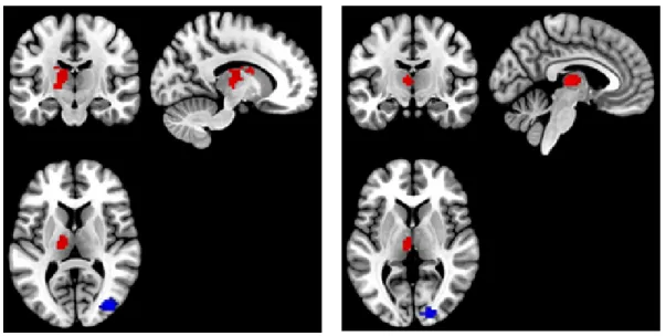
Two canonical ROIs were chosen from the previous GLM analysis (Thalamus and Occipital Lobe) (Laufs et al., 2003), both for eye closed and open conditions, under individual voxel p-value≺10−6_{, cluster size50. A positive correlation between BOLD and canonical HRF}

convolved alpha power was observed in the thalamus, and a negative one in the Occipital Lobe (Figure 2.7). After (canon2dd and sFIR) HRF deconvolution, the Pearson correlation between devonvolved BOLD and alpha power is almost strengthened, only one weaken connectivity is found in thalamus with eye closed after canon2dd HRF deconvolution (Figure 2.8). The voxel-level HRF shapes derived in these two regions in the two conditions are reported in Figure 2.9. We observed opposite patterns of HRF shapes between the thalamus and occipital cortex under the two conditions, which is consistent with the correlation and anti-correlation between the alpha power spectrum and BOLD signal in thalamic and occipital cortex. It is worth noting how the variations in HRF are consistent with the differences in net arterial and venous flow, and the consequent effects on the estimation of Granger causality reported in (Webbet al., 2013). This evidence confirms the importance of performing HRF deconvolution prior to estimating not only for lag-based directed connectivity (Wu et al., 2013a), but also for standard functional connectivity.

Retrieving the HRF in rs-fMRI

2

2.3.4

HRF modulations with eyes open and closed

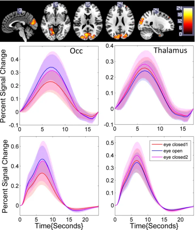
In order to study the modulations of HRF shape when opening or closing the eyes on a larger sample, we considered a dataset of 48 healthy controls collected at the Beijing Normal University in China with 3 resting state fMRI scans of six minutes each (http://fcon_1000.projects.nitrc.org/indi/IndiPro.html). During the first scan participants were instructed to rest with their eyes closed. The second and third resting state scan were randomized between resting with eyes open versus eyes closed. Data were preprocessed as described in the above section. Then the resting state HRF was retrieved. Statistical significance of the spontaneous hemodynamic response evoked by opening and closing eyes was assessed with a group-level repeated-measures analysis of covariance (ANCOVA) that included subjects as the random factor and two fixed factors, resting state type (eyes closed and open) and order (eyes closed-open-closed, eyes closed-closed-open), age, gender, and mean framewise displacement (FD) power as the covariates. The ANCOVA revealed significant main effect for resting state conditions (eye closed/open) in hemodynamic response height. No significant main effect of order and interaction effect were found. The significant differences in the height of the HRF located in the occipital areas, which were depicted in figure 2.10. The corresponding HRF shape is also reported. Though the difference in the thalamus is not obvious, we still can find the opposite patterns of HRF shapes under eye closed and open, similar with the finding in EEG-fMRI dataset.

2.3.5

HRF variability

The hemodynamic response has been shown to vary in timing, amplitude, and shape across brain regions and cognitive task paradigms (Miezin et al., 2000; Handwerker et al., 2012a; Badillo et al., 2013). Such variation is expected also for resting state. In order to investigate the variability on the resting state HRF, test-retest (TRT) reliability analyses were performed on a resting-state fMRI dataset that has been publicly released in the ’1000 Functional Connectomes Project’. All included participants had no history of neurological and psychiatric disorders and all gave the informed consent approved by local Institutional Review Board. During the scanning participants were instructed to keep their eyes closed, not to think of anything in particular, and to avoid falling asleep. Two data sets with different TR (TR = 2.5 s and TR = 0.645 s) were acquired on Siemens 3T Trio Tim scanners using standard EPI sequence (TR = 2500msec, 3mm isotropic voxels, 5 minutes) and multiband EPI sequence (TR = 0.645 s, 3 mm isotropic voxels, 10 min). To evaluate the test-retest reliability of the voxel HRF parameters between the two sessions, a measurement of the intraclass correlation coefficient (ICC) was employed. A one-way ANOVA with random subject effect was used to compute the between-subject mean square (BMS) and within-subject mean square (WMS). Then an ICC(3,1) value was subsequently

2

ICC = BM S−W M S

BM S+ (m−1)W M S (2.4)

wherem represents the number of repeated measurements of the voxel HRF parameter (here, m = 2). We calculated the ICC value for each voxel and generated the ICC map for each HRF parameter. Next, the TRT reliability of the HRF parameter was assessed in a voxel-wise manner with the classifying criteria of ICC values (Sampat et al., 2006): less than 0.4 indicated low reliability; 0.4 to 0.6 indicated fair reliability; 0.6 to 0.75 indicated good reliability and 0.75 to 1.0 indicated excellent reliability. To further assess the regional variability of TRT reliability, we utilized the above-mentioned prior functional parcellation of cerebrum, and calculated the mean ICC values and their standard deviations within these subnetworks, respectively. As was expected, sFIR showed lower ICC than canon2dd model, both at voxel level and large-scale network level. We did not observe an obvious spatial pattern in the ICC maps for distinct networks (Figures 2.11-2.12). The hemodynamic response height (PSC) showed good reliability for canon2dd model acorss all subnetworks and TR (excluding the VN at TR=2.5s), and for sFIR in VAN, FPN and DMN at TR=2.5s, and fair reliability for most of the subneworks with sFIR model (Figure 2.11). The other HRF parameters (FWHM and time to peak) showed low reliability. These results reveal that the different hemodynamic response sampling (i.e. in units of TR) only slightly affects the ICC maps of hemodynamic response height.

2.4

Conclusions and future work

We have presented a methodology to retrieve the hemodynamic response function from resting state fMRI data. The feasibility and effectiveness of proposed algorithm is con-firmed by simulation data. The results are promising since the retrieved HRF is consistent with the literature and supports evidences of the vascular flow. Additionally, functional modifications to the HRF shape are consistent with evidence previously reported using dif-ferent methodologies. The approach will need further validation using electrophysiological and cardiovascular data.

(a)

(b)

(c)

Figure 2.2: shows (a) ER stimulus timing, the ideal BOLD response, and ideal response corrupted with noise (SNR=1) (b) Ground truth (Balloon) and estimated HRFs for fixed ISI ER design, (c) Ground truth and estimated HRFs for jittered ER design. The colored shadow indicates the standard deviation.

2

(a)

Retrieving the HRF in rs-fMRI

2

(b)

Figure 2.3: Median maps of CBF and HRF parameters across subjects. Page 26

2

Figure 2.4: Scatterplot of the spatial correlations across voxels between CBF and HRF parameters. X-axis is the CBF, Y-axis are the HRF parameters. Blue scatterplot indicate the linear correlation is significant,p≺0.05 corrected.

Retrieving the HRF in rs-fMRI

2

Figure 2.5: Scatterplot of the across subject correlations between CBF and HRF parameters. X-axis is the CBF, Y-axis are the HRF parameters. Blue scatterplots indicate the linear correlation is significant,p≺0.05 corrected.

2

Figure 2.6: Correlations between CBF and HRF parameters at voxel level across subjects. The upper colorbar is for inside plots, the bottom colorbar is for surface plots.

Retrieving the HRF in rs-fMRI

2

Figure 2.7: clusters of significant correlation (red) and anti-correlation (blue) between BOLD and alpha power spectrum

Figure 2.8: Pearson correlation between (BOLD) Deconvolved BOLD signal and (canonical HRF convolved) alpha power. Occ: occipital area; Thal: thalamus; Cc: eyes closed, canon2dd; Cs: eyes closed, sFIR; Oc: eyes open, canon2dd; Os: eyes open, sFIR.

2

Figure 2.9: HRF at rest in the occipital cortex (left) and in the thalamus (right) for eyes open and closed. Left upper pannel is HRF estimated by sFIR model, the bottom pannel is HRF estimated by canonical HRF with its derivatives. The red and blue shadows are the standard deviations of voxelwise HRFs under eyes closed and open conditions.

Retrieving the HRF in rs-fMRI

2

Figure 2.10: Statistical differences in HRF height with eyes closed (1), open, then closed again (2) (top), and typical shapes in the occipital (left) and thalamic (right) area (middle: sFIR;

bottom: canonical HRF with its derivatives).

2

Figure 2.11: TRT reliability of HRF parameters within seven subnetwork. C-TR645: canon2dd HRF, TR=0.645s; S-TR645: sFIR HRF, TR=0.645s; C-TR25: canon2dd HRF, TR=2.5s; S-TR25: sFIR HRF, TR=2.5s; T2P: Time to peak.

Retrieving the HRF in rs-fMRI

2

Figure 2.12: TRT reliability maps of hemodynamic response height (PSC) with different HRF basis vector s(canon2dd, sFIR), at different TR (0.645s, 2.5s).

3

Modulated spontaneous hemodynamic response to loss of

consciousness

Abstract

Functional imaging has already accumulated abundant research results on the neural correlates of consciousness. Apart from task-related activation derived in fMRI, PET based glucose metabolism rate or cerebral blood flow account for a considerable proportion in the study of brain activity under different level of consciousness. Resting state functional connectivity MRI is playing a crucial role to explore the consciousness related functional integration. So far, a comparatively comprehensive and systematic comparison of brain activity measured by PET and BOLD-fMRI in the resting state has never been done. Here, spontaneous hemodynamic response is introduced to characterize resting state brain activity, then used to investigate the loss of consciousness under propofol anesthesia and vegetative state. The previous PET results on anesthesia or pathology induced loss of consciousness are validated by resting state hemodynamic response. The dysfunction of hemodynamic response in precuneus and posterior cingulate is found to be a common principle underlying loss of consciousness in both conditions. The thalamus appears to be less obviously modulated by propofol, compared with frontoparietal regions. However, a significant reduction in spontaneous thalamic hemodynamic response was found in vegetative state.

Modulated spontaneous hemodynamic response to loss of consciousness

3

3.1

Introduction

It is crucial to understand the physiologic basis of consciousness in pathological or pharma-cological coma, which may provide effective assistance to diagnosis, prognostication, and assess potential treatments. The advanced neuroimaging techniques have significantly ex-panded our knowledge of neural correlates of conscious level in human brain. For instance, FDG-PET imaging and fMRI have shown that altered metabolism and connectivity in thalamus, frontoparietal and default mode network (Laureys, 2005; Laureys et al., 2000a,b, 2002, 2004) are found in patients with disorders of consciousness, electrophysiological techniques have discovered some covert rhythm signs of consciousness (Gugino et al., 2001; Vijayan et al., 2013). Finding high test-retest reliable evidences within or across multi-mode imaging are the necessary step to obtain the clinically applicable neural markers of consciousness. Such work has gained extensive attention and not confined to consciousness, especially in the fMRI studies (Plichta et al., 2012). A clinical validation study reveals that PET imaging show higher diagnostic precision than fMRI in disorders of consciousness (Stender et al., 2014). This indicates much more underlying dynamic information mining should be explored with advanced fMRI model, considering that spatiotemporal resolution is more excellent with fMRI than PET.

Consciousness has two major components: awareness of environment and of self (i.e. the content of consciousness) and wakefulness (i.e. the level of consciousness) (Laureys, 2005). The vegetative state is the most tragic model that dissociates wakefulness and awareness. The accumulated neuroimaging evidences revealing how them could be separated in vegetative state (VS), mainly deriving from the correlation between awareness and global brain function (Laureys et al., 1999a), regional brain function, brain activation induced by passive external stimulation (Laureys and Schiff, 2012) or mental imagery task (Owenet al., 2005), changes in resting state connectivity (Laureyset al., 2000b, 1999a,b). While the anesthetic drugs manipulation to achieve specific state of consciousness is another direct way to explore qualitative nature of consciousness (Alkire and Miller, 2005), similar brain imaging techniques as applied in VS are used to identify neural correlates of consciousness (Boveroux et al., 2010; Hudetz, 2012; DiFrancescoet al., 2013). Compare to global brain metabolism, regional metabolic dysfunction is a more reliable maker of individual conscious-unconscious state transition (Laureys, 2005). The studies of passive stimuli have shown promising results, especially for minimally conscious state patients, but the neuronal responses cannot be always stable (Laureys and Schiff, 2012) then the followed inference of cognitive function from these cerebral activations is controversial (Menon et al., 1999; Schiff and Plum, 1999). Resting state functional connectivity (FC) play a critical role in the quantification of brain function integration that maintaining the state of consciousness (Laureys et al., 2000b, 1999a,b; Boverouxet al., 2010), and well confirmed the previous FDG-PET results (Laureys and Schiff, 2012). Nevertheless, brain connectivity are now Page 36

3

and motion artifact (Power et al., 2012) may contribute high proportion to observed FC. BOLD-fMRI hemodynamic response describe the vascular oxygenation changes to a neuronal impulse response, is a more relevant measure of neural activity with PET. To validate and confirm the cerebral metabolic patterns of altered level of consciousness observed in PET studies from a different neuroimaging technique, we investigate the hemodynamic response pattern in VS patient and the healthy subjects with propofol anesthesia using resting state fMRI data. The hemodynamic response correlates of consciousness will be explored and compared between vegetative state and anesthesia. According to the previous PET studies (Bolyet al., 2011; Laureys, 2005; Laureys et al., 2004), we hypothesis thalamus, fronto-parietal cortical areas and default mode network (DMN) will exhibit state-dependent spontaneous hemodynamic response in the resting

state.

3.2

Materials and Methods

3.2.1

Subjects

Twenty-one healthy right-handed volunteers, twenty coma patients and thirty two healthy controls participated in the study. The subjects provided written informed consent to participate in the study. None of the healthy subjects had a history of head trauma or surgery, mental illness, drug addiction, asthma, motion sickness, or previous problems during anesthesia. The study was approved by the Ethics Committee of the Medical School of the University of Liege (University Hospital, Liege, Belgium).

3.2.2

Functional Data Acquisition

The propofol dataset considered in current study has already been published in (Boveroux et al., 2010). Functional MRI acquisition consisted of resting-state fMRI volumes repeated in four clinical states only for 21 healthy volunteers: normal wakefulness (W1), mild sedation (S1), deep sedation (S2), and recovery of consciousness (W2). The temporal order of mild- and deep-sedation conditions was randomized. The typical scan duration was half an hour in each condition. The number of scans per session was matched in each subject to obtain a similar number of scans in all four clinical states (mean ± SD, 251 ± 77 scans/session). There is only one session of resting state fMRI for each subject in VS dataset, each one contains 297 scans. All functional images were acquired on a 3 Tesla Siemens Allegra scanner (Siemens AG, Munich, Germany);

• Propofol dataset: Echo Planar Imaging sequence using 32 slices; repetition time (TR)=2460ms, echo time=40ms, field of view = 220mm, voxel size=3.45×3.45×3 Page 37

Modulated spontaneous hemodynamic response to loss of consciousness

3

mm, and matrix size=64×64×32).

• VS dataset: Echo Planar Imaging sequence using 32 slices; repetition time (TR)=2000ms, echo time=30ms, field of view = 384mm, voxel size=3.44×3.44×3 mm, and matrix size=64×64×32).

3.2.3

Data Preprocessing

All structural images in both datasets were manually reoriented to the anterior commissure and segmented into grey matter, white matter (WM), cerebrospinal fluid (CSF), skull, and soft tissue outside the brain, using the standard segmentation option in SPM 12. Then a DARTEL template was created based on the deformation fields that are produced during the segmentation procedure. Resting-state fMRI data preprocessing was subsequently carried out using both AFNI and SPM12b package. First, the EPI volumes were corrected for the temporal difference in acquisition among different slices, and then the images were realigned to the first volume for head-motion correction. 8 VS patients and 7 healthy control subjects were excluded from the dataset because either translation or rotation exceeded ±1.5 mm or ±1.5◦, or mean framewise displacement (FD) exceeded 0.3, resulting in 12 VS patient and 25 healthy controls which were used in the analysis, and 22 sessions in propofol group sub