HAL Id: hal-01322374
https://hal.archives-ouvertes.fr/hal-01322374v2
Submitted on 21 Jun 2017
HAL
is a multi-disciplinary open access
archive for the deposit and dissemination of
sci-entific research documents, whether they are
pub-lished or not. The documents may come from
teaching and research institutions in France or
abroad, or from public or private research centers.
L’archive ouverte pluridisciplinaire
HAL, est
destinée au dépôt et à la diffusion de documents
scientifiques de niveau recherche, publiés ou non,
émanant des établissements d’enseignement et de
recherche français ou étrangers, des laboratoires
publics ou privés.
Tail dimension reduction for extreme quantile estimation
Laurent Gardes
To cite this version:
Laurent Gardes. Tail dimension reduction for extreme quantile estimation. Extremes, Springer Verlag
(Germany), 2018, 21 (1), pp.57-95. �hal-01322374v2�
Tail dimension reduction for extreme quantile estimation
Laurent Gardes
Université de Strasbourg, CNRS, IRMA UMR 7501,
F-67000 Strasbourg, France.
Abstract
In a regression context where a response variableY ∈Ris recorded with a covariateX∈Rp,
two situations can occur simultaneously: (a) we are interested in the tail of the conditional distribution and not on the central part of the distribution and (b) the numberpof regressors is large. To our knowledge, these two situations have only been considered separately in the literature. The aim of this paper is to propose a new dimension reduction approach adapted to the tail of the distribution in order to propose an efficient conditional extreme quantile estimator when the dimensionpis large. The results are illustrated on simulated data and on a real dataset.
Keywords−Regression, extreme quantile, dimension reduction, kernel smoothing.
AMS Subject classifications−62G32, 62G08, 62G05, 62G20.
1
Introduction
This work takes place in a regression context where a real response variableY is recorded with a
random vectorX ∈E⊂Rpof explanatory variables. In the literature, several ways for examining
how the distribution ofY is influenced by the regressorX have been considered. The most
com-mon approach summarize the relationship between Y and X by the regression functionE(Y|X)
which is the conditional expectation ofY given X. Several estimators of the regression function
are available, the probably most known being the kernel estimator introduced independently by Nadaraya [29] and Watson [35]. In the same spirit, one can also mention the estimator introduced
by Gasser and Müller [20]. Another way to understand the link between Y and X is to use a
conditional quantile of fixed order1−α∈(0,1). For instance, Koenker and Basset [26] introduced
the notion of quantile regression assuming that the conditional quantile ofY given X is a linear
combination of the explanatory variables. This approach has the advantage of being more robust against outliers than the regression function. Concerning the estimation of conditional quantile, local linear approaches were considered by Yu and Jones [39] while a fully nonparametric estimator can be found in the paper of Chaudhuri [3].
In many applications such as climatology, finance, insurance to name a few, two situations can occur simultaneously in a regression context.
(a) We are interested in the tail distribution of Y given X instead of the central part of the
conditional distribution. In this case, regression function and conditional quantile of fixed order
(b) The dimension p of the regressor is large. In this situation, inference on the conditional
distribution ofY given X becomes difficult since the space is sparsely populated by data points.
This is the well known curse of dimensionality problem.
A motivating example is the study of the influence of various pollutants (sulphur dioxide, nitrogen dioxide, carbon monoxide, . . . ) and weather conditions (temperature, humidity, . . . ) on extreme values of ozone concentration (see Section 5). Another example can be found in hydrology where the understanding of the influence of the geographical position and the altitude on return periods of large amount of rain is a problem of primary interest (see Gardes and Girard [17]). Despite this large range of applications, situations (a) and (b) mentioned before have been considered sep-arately in the literature.
To make inference on the tail distribution of Y given X, one solution is to use a conditional
quantile of order1−αnwhereαn→0as the sample sizengoes to infinity. Such a quantile is said
to be extreme. Estimation of conditional extreme quantiles has been considered by many authors. One common approach consists to fit a parametric model for exceedances over a high threshold (see Davison and Smith [9] and Northrop and Jonathan [30]). In Davison and Ramesh [10], a local likelihood smoothing procedure is considered for the estimation of a conditional generalized extreme value distribution and Eastoe and Tawn [12] propose to model the covariate effect by a
Box-Cox location-scale model. A nonparametric estimation procedure is proposed by Daouiaet
al.([7] and [8]) and Gardes and Girard [18].
To deal with high dimensional covariates, a classical method is to assume the existence of a
p×q full rank matrix B (with q < p) such that the conditional distributions of Y given B>X
and Y given X are the same. In others words, it is assumed that X and Y are independent
conditionally onB>X (in symbols X
|
=Y|B>X). For a comprehensive discussion on conditional
independence see Basu and Pereira [2]. In the literature, this model is referred to the
multiple-index model (single-multiple-index model ifq= 1) and the subspace spanned by the columns ofB is called
the Dimension Reduction (DR) subspace. Among the contributions on the estimation of the DR subspace, one can cite the Sliced Inverse Regression (SIR) method introduced by Li [27], the Slice Average Variance Estimation (SAVE) method proposed by Cook and Weisberg [6] and the Princi-pal Hessian Directions (PHD) method (see Li [28]). The existence of a DR subspace is assumed by
many authors in order to study the link betweenY and the explanatory variablesX. For instance,
to estimate conditional quantiles of fixed order, Wu et al. [37] use a single-index model while a
combination of SIR and kernel estimation is considered by Gannounet al.[15].
To our knowledge, the use of adapted dimension reduction methods for estimating conditional extreme quantiles has not been considered yet in the literature. One can mention the recent paper
of Russelet al.[32] where the relationship betweenY andX is summarized by the link betweenY
and a linear combination of the explanatory covariates. This combination is obtained by optimizing the tail dependence with the response variable. Note that this method is based on the assumption
that the random vector(X, Y)is regularly varying while no particular condition onX is required
in our approach.
In the present paper we first adapt the classical definition of conditional independence to an ex-treme value context. More specifically, we introduce the notion of Tail Conditional Independence
(TCI) of Y and X given Z. Roughly speaking, TCI means that the tail distribution of Y given
(X, Z)is asymptotically equivalent to the one ofY givenZ. This new definition permits us to deal
Next, the notion of Tail Dimension Reduction (TDR) subspace is introduced. The TDR subspace
is spanned by ap×q full rank matrix B such that Y and X are tail conditionally independent
given B>X. Note that for any regular q×q matrix D, the subspace spanned by B is also the
subspace spanned by BD. To avoid this misspecification issue, the matrixB spanning the TDR
subspace is taken in the set B where B ∈ B if the q columns of B are the first normalized q
linearly independent columns of the orthogonal projection matrix on the subspace spanned byB.
Taking advantage of the existence of a TDR subspace, a kernel-based statistic is then proposed as a first estimator of conditional extreme quantiles. Unfortunately, this estimator is only of
theoret-ical interest since it depends on the unknown directionB of the TDR subspace. Estimation ofB
is thus considered leading to the definition of a more useful conditional extreme quantile estimator.
The paper is organized as follows. Tail Conditional Independence and Tail Dimension Reduc-tion subspace are defined in SecReduc-tion 2. In SecReduc-tion 3, assuming the existence of a Tail Dimension Reduction subspace, the estimation of conditional extreme quantiles is addressed. Finite sample properties are investigated through a simulation study in Section 4. Note that, due the
compu-tational cost in the estimation ofB when q > 1 (see end of Section 3.2), only the case q = 1is
considered. Our estimation procedure is applied to study the influence of various pollutants on ozone concentration in Section 5. Proofs are postponed to the appendix.
2
Tail Conditional Independence and Tail Dimension
Reduc-tion subspace
2.1
Definition of Tail Conditional Independence
Let(X, Y, Z) ∈Rp×R×Rq be a random vector defined on a probability space (Ω,F,P). The
goal of this section is to introduce the notion ofTail Conditional Independence (TCI) of Y and
X given Z. First, let us give some notations used in all what follows. For any random variable
W : (Ω,F,P)7→(Rm,B(Rm))wherem∈N∗, letsupp(W)be the support of its distribution. We
denote by P(·|W = ·) : F ×supp(W) 7→ [0,1] a regular version of the conditional expectation
E(I{·}|W)where the dot denotes any element ofF andI{·} is the indicator function. Finally, the
conditional quantile ofY given W of orderα∈[0,1]is the measurable functionQ(α|W =·) :=
inf{y ∈ R; P(Y > y|W = ·) ≤ α} where R denotes the extended real number line. The TCI property is defined below.
Definition 1. The random variable Y is tail conditionally independent ofX givenZ (in symbols
Y∼|=X|Z) if for all ε >0there existsκ >0 such that for all δ∈(0, κ],
P P(Y >Yδ(Z)|X, Z) P(Y >Yδ(Z)|Z) −1 ≤ε = 1, (1)
where forδ >0,Yδ(Z=·)is a measurable function defined onsupp(Z)and given byYδ(Z =·) :=
Q(0|Z=·)−δ ifQ(0|Z=·)<+∞and Yδ(Z=·) :=δ−1 ifQ(0|Z =·) = +∞.
Note that, as a direct consequence of (1), ifY ∼|=X|Z then Q(0|X, Z) =Q(0|Z)a.s. that is to say
that the distributions ofY given(X, Z)andY givenZ share the same right endpoint.
setA ∈ B(Rp)⊗ B(
Rq)withP[(X, Z)∈ A] = 1such that for all(x, z)∈ A, lim
y↑Q(0,Z=z)
P(Y > y|X =x, Z=z)
P(Y > y|Z=z) = 1. (2)
Hence, ifY ∼|=X|Z, the conditional tail distribution ofY given(X, Z)is asymptotically equivalent
to the one ofY givenZ and thus, inference on the tail ofY given(X, Z)can be achieved without
the information carried byX. This property can be of high interest in practice if the dimension
ofZ is much smaller than that ofX (see the next section).
The TCI property is obviously less restrictive than the classical conditional independence property
since the last one assumes that P(Y > y|X, Z) =P(Y > y|Z)a.s. for ally ∈R. Note also that
the conditional independence property is symmetric (i.e. X |=Y|Z ⇔Y |=X|Z) but not the tail
conditional independence property.
As it is the case for the conditional independence property, the TCI property can be characterized in different equivalent ways. This is the purpose of the next result.
Theorem 1. The following statements are equivalent:
(i)Y∼|=X|Z.
(ii) For allε >0 there exists κ >0 such that for all δ∈(0, κ] and for all non-zero bounded and positive measurable functionh(·),
P E(I{Y >Yδ(Z)}h(X)|Z) P(Y >Yδ(Z)|Z)E(h(X)|Z) −1 ≤ε = 1.
(iii) For all δ >0,P(Y >Yδ(Z)|X, Z) = sδ(Z)(1 +ηδ(X, Z))a.s., where sδ : supp(Z)7→R and
ηδ : supp(X, Z)7→Rare two measurable functions and, for all ε∈(0,1), there exists κ >0 such
that for allδ∈(0, κ],P[|ηδ(X, Z)| ≤ε] = 1.
Note that uniform convergence in (1) (i.e. the fact thatκ does not depend on the values of the
random vector(X, Z)) is essential to prove the second and third statements in Theorem 1.
Further-more, since the conditional expectation is almost surely unique, Theorem 1 can not be established if we ask that (2) holds everywhere.
The second statement gives us another way to understand the TCI property. It entails that
for all bounded and positive measurable functionh(·), there exists a Borel set A ∈ B(Rq) with
P(Z ∈ A) = 1such that for allz∈ A,E I{Y >y}h(X)
Z=z
∼P(Y > y|Z =z)E(h(X)|Z=z) asy↑Q(0|Z =z). In the particular situation considered later whereZ=B>X withBa full rank
p×qmatrix (q < p), this property will be the starting point for the estimation ofB.
The third statement is a very useful tool for anyone who wants to propose conditional distributions
ofY given(X, Z)satisfying Definition 1. Some examples are given hereafter.
Example 1. Letµ1(·|(X, Z) =·) :B(R)×supp(X, Z)7→([0,1],B([0,1]))andµ2(·|Z =·) :B(R)×
supp(Z)7→([0,1],B([0,1])) be two functions such that for all (x, z)∈ supp(X, Z),µ1(·|(X, Z) =
(x, z)) and µ2(·|Z = z) are two probability measures on (R,B(R)) and, for all A ∈ B(R), the
functionsµ1(A|(X, Z) =·)andµ2(A|Z=·)are measurable. We assume in addition that uniformly
on(x, z)∈supp(X, Z), lim δ→0 µ1(Iδ(z)|(X, Z) = (x, z)) µ2(Iδ(z)|Z =z) = 0.
whereIδ(z) = [Yδ(Z =z),∞). Regardless of the distribution of(X, Z), if the conditional
distri-bution ofY given(X, Z)is the mixture distribution defined by
P(Y ∈ ·|X, Z) =θ(Z)µ1(·|X, Z) + (1−θ(Z))µ2(·|Z)a.s.,
whereθ(·)is a [0,1)−valued measurable function, then, from Theorem 1 point (iii), it is easy to
see thatY ∼|=X|Z.
Example 2. Consider the semi-parametric model
P(Y > y|X) =y−exp(b
>
0X)L(y|X)a.s.,
whereb0 ∈Rp and L(·|X =·) : R×supp(X)7→(0,∞)is a function such that for all t >0 and
x∈ supp(X), L(ty|X = x)/L(y|X = x) → 1 as y → ∞. Note that this model was introduced
by Wang and Tsai [34] where a maximum likelihood method to estimateb0 is considered. If we
assume thatL(y|X=x)converges toc(b>0x)uniformly onx∈supp(X)asy→ ∞where c(·)is a
positive and measurable function then, using the third statement of Theorem 1, it is easy to check
thatY ∼|=X|b>0X.
2.2
Tail Dimension Reduction subspace
Using the notion of Tail Conditional Independence presented in the previous section, we give now
the definition of a TDR subspace. In what follows, for a full rankp×qmatrixB withq < p, the
space spanned by the columns ofB is denoted S(B).
Definition 2. If there exists a full rankp×q matrix B0 ∈ B with q < p such that Y ∼|=X|B0>X
thenS(B0)is a Tail Dimension Reduction (TDR) subspace forY givenX.
The TDR subspace is an adaptation of the DR subspace introduced by Li [27]. Recall that since
B0 ∈ B, the matrix B0 spanning the TDR subspace is unique. In particular its columns are
orthogonal unit vectors. Roughly speaking, if there exists a TDR subspaceS(B0), the tail of the
conditional distribution ofY givenX can be reasonably approximated by the tail of the conditional
distribution ofY given B0>X. Obviously, for any random vector (X, Y), S(Ip) = Rp is a TDR
subspace and thus a TDR subspace is not unique. Since our goal is to reduce the dimension, the
notion ofminimum TDR subspaceis defined below by analogy with the definition of the minimum
DR subspace (see for instance [4]).
Definition 3. For a full rank matrixB0∈ B, the subspaceS(B0)is a minimum TDR subspace if
its dimension is less than or equal to the dimension of any other TDR subspace.
3
Extreme quantile estimation under a TDR model
Let(X, Y)∈Rp×Rbe a random vector defined on the probability space(Ω,F,P). In what follows,
the distribution of(X, Y) is assumed to be absolutely continuous with respect to the Lebesgue
measure. A probability distribution function ofX is denoted byfX(·)and its support is given by
supp(X) :={x∈Rp; fX(x)>0} which is assumed to be an open set.
The aim of this section is to propose an estimator of the conditional quantileQ(α|X) whenαis
close to 0 (conditional extreme quantile) and when the dimension pof the covariate X is large.
investigated by several authors (see for instance Araújo Santoset al.[1], Daouiaet al. [7], Gardes and Girard [18] among many others). Unfortunately, these estimators often fail to approximate correctly the conditional extreme quantile in a large dimension setting since in this situation, the
spacesupp(X)is only sparsely populated by data points. As a consequence, only few points can be
reasonably considered to estimateQ(αn|X =x)and, unless the sample size is very large, classical
estimators become inefficient for large values ofp.
In this section, the existence of a minimum TDR subspaceS(B0) is assumed and a new kernel
estimator ofQ(αn|X =x)is proposed. This new estimator is expected to be more efficient than
classical kernel estimators for large values ofp. In a preliminary step (see Section 3.1), we introduce
a statisticQbn(αn|B0, x)depending on the unknown direction B0 and which is consistent for the
estimation ofQ(αn|X =x). Obviously, this statistic is useless since in practice B0 is unknown.
An estimator ofB0is thus proposed in Section 3.2 and the estimation ofQ(αn|X =x)is achieved
by replacing the true directionB0 by its estimated version inQbn(αn|B0, x).
3.1
Conditional extreme quantile estimation: the case
B
0known
Givennindependent copies(X1, Y1), . . . ,(Xn, Yn)of the random vector(X, Y), we are interested in
the estimation of the conditional extreme quantileQ(αn|X =x)forx∈supp(X)whereαn∈(0,1)
converges to 0 asngoes to infinity.
The first step is the estimation of the conditional survival function P(Y > y|X = x) for large
values ofy. Assuming the existence of a minimum TDR subspaceS(B0), the conditional survival
functionP(Y > y|X=x)can be approximated fory large enough byP(Y > y|B0>X =B>0x). We
thus propose the following statistic as an estimator ofP(Y > y|X=x):
b Sn(y|B0, x) := n X i=1 I{Yi>y}K H −1 n B > 0(x−Xi) , n X i=1 K Hn−1B0>(x−Xi) . (3)
Here, Hn is a sequence of q×q positive definite matrices and K(·) is a probability distribution
function onRq. From now on, we assume thatK(·)is bounded with support the unit ball of
Rq.
Note thatSbn(y|B0, x)is the classical kernel estimator ofP(Y > y|B>0X=B0>x)that is considered
here as an estimator ofP(Y > y|X =x).
A first attempt to estimateQ(αn|X=x)is to use the generalized inverse ofSbn(·|B0, x)leading to
the statistic
b
Qn(αn|B0, x) := inf{y; Sbn(y|B0, x)≤αn}. (4)
Unfortunately, such an estimator fails to estimate extreme quantiles of orderαnas small as we like.
Indeed, it is shown in Proposition 4 that the conditionn|Hn|αn → ∞, where|Hn|stands for the
determinant ofHn, is required to establish the consistency of (4). As a consequence,Q(αn|X =x)
cannot be consistently estimated by (4) whenαn is too small. To overcome this drawback,
addi-tional information on the tail distribution ofY givenX is necessary.
Extended regular variation. In the unconditional case, when dealing with the right-tail of
a real random variable Y, it is commonly assumed that Y belongs to the maximum domain of
attraction of an extreme value distribution (see Fisher and Tippett [13] and Gnedenko [21] for a definition). According to de Haan and Ferreira [22, Theorem 1.1.6], this is equivalent to assuming
the existence of a positive auxiliary functionaY(·)and a parameterγY ∈Rsuch that for allu >0,
for allv ≥1 and s∈R, Ls(v) :=Rv
1 u
s−1du. The function Q
Y(·) is then said to be of extended
regular variation.
The same kind of assumption is made in our conditional setting. We assume that for all x ∈
supp(X), the function Q(·|X =x)is of extended regular variation i.e. that there exist a positive
functiona(·|x) : (0,∞) 7→ (0,∞) and a real-valued function γ(·) such that for all x∈ supp(X)
andu >0, ERV(α, u|x) := Q(uα|X=x)−Q(α|X =x) a(α−1|x) −Lγ(x)(1/u) →0, (5) asα→0. Note that this convergence holds locally uniformly onu∈(0,∞). The function γ(·)is
referred to as the conditional extreme value index function. The functiona(·|x), called the auxiliary
function, is such thata(α−1|x)/Q(α|X =x)−γ
+(x)→0 as αgoes to 0 where(·)+ and(·)− are
the positive and negative part functions (see Fraga Alveset al. [14, Lemma 3.1]). Condition (5)
is equivalent to assuming that the distribution functionP(Y ≤ ·|X =x)belongs to the maximum
domain of attraction of an extreme value distribution with extreme value indexγ(x). Condition (5)
is also satisfied for the conditional quantile ofY givenB0>X as it is shown in the following result.
Proposition 1. Let B0 ∈ B be a full rank matrix such thatS(B0) is a TDR subspace. If for all
x∈supp(X), the conditional quantile Q(·|X =x) satisfies (5), there exist a Borel setA ∈ B(Rp)
withP(X ∈ A) = 1, a positive functiona˜(·|B0>x) and a real-valued functionγ˜(·)such that for all u >0 andx∈ A, lim α→0 Q(uα|B0>X =B>0x)−Q(α|B0>X=B>0x) ˜ a(α−1|B> 0x) =L˜γ(B> 0x)(1/u).
In addition, for allx∈ A,γ(x) = ˜γ(B0>x)and˜a(α−1|B>
0x) =a(α−1|x).
To estimateQ(βn|X=x)for an arbitrary sequence(βn)converging to 0, we start with (5) which
suggests the approximationQ(βn|X =x)≈Q(αn|X =x) +a(α−n1|x)Lγ(x)(αn/βn). The sequence
(αn) is chosen not too small so that Q(αn|X = x) can be consistently estimated by the kernel
estimatorQbn(αn|B0, x)defined in (4). Assuming as before that S(B0) is a TDR subspace for a
given full rank matrixB0, an estimator ofQ(βn|X=x)is thus given by
ˇ
Qn(βn|B0, x) :=Qbn(αn|B0, x) +ban(B0, x)L
b
γn(B0,x)(αn/βn), (6)
wherebγn(B0, x)and ban(B0, x)are consistent estimators of γ(x)anda(α
−1
n |x). Before giving the
expression of these two estimators, let us introduce some notations. For ν ∈ (0,1) and ϕ(·) a
positive and bounded function on[ν,1], letΨ(·)be the decreasing function defined for s≥0 by
Ψ(s) = 0and fors≤0by Ψ(s) := Z 1 ν ϕ(u)Ls(1/u)du 2Z 1 ν ϕ(u)L2s(1/u)du .
The function Ψ←(·) given by Ψ←(t) = inf{s; Ψ(s) ≤ t} is the generalized inverse of Ψ(·). In
addition, for allδ∈N, for all non-increasing right-continuous function U(·)and allα∈(0,1), let
T(δ) α (U) := Z 1 ν ϕ(u) lnU(uα) U(α) δ du , Z 1 ν ϕ(u)L0(1/u)du δ .
The estimatorbγn(B0, x)is given by
b γn(B0, x) := bγn,+(B0, x) +bγn,−(B0, x) = T(1) αn(Qbn(·|B0, x)) + Ψ ← [T (1) αn(Qbn(·|B0, x)]2 Tα(2)n(Qbn(·|B0, x) ! . (7)
Note that this estimator belongs to the class of estimators introduced in Gardes [16]. Concerning
the estimation ofa(α−n1|x), we consider the statistic
b an(B0, x) =Teαn b Qn(·|B0, x);bγn,−(B0, x) , (8)
whereTeα(U, γ−)is given for all non-increasing and right-continuous functionU(·), for allγ−≤0
and for allα∈(0,1)by
e Tα(U, γ−) :=U(α) Z 1 ν ϕ(u) lnU(uα) U(α) du Z 1 ν ϕ(u)Lγ−(1/u)du .
Note that the previous defined estimators depend on the choice of a parameter ν ∈ (0,1) and a
positive and bounded functionϕ(·)on[ν,1]. In order to not overload the notations, this dependence
has been omitted. Expressions ofbγn(B0, x)andban(B0, x)are motivated by the following result.
Proposition 2. Let x∈supp(X). If condition (5) holds then
lim α→0T (1) α (Q(·|X =x)) =γ+(x), lim α→0 [Tα(1)(Q(·|X =x))]2 Tα(2)(Q(·|X =x)) = Ψ(γ−(x)), and lim α→0 e Tα(Q(·|X =x), γ−(x)) a(α−1|x) = 1.
The proof of this Proposition is a direct consequence of [16, Lemma 3]. Its proof is thus omitted.
The study of the asymptotic behavior ofQˇn(βn|B0, x)is done under the assumptions given below.
Condition on the TDR subspace. Recall that, from Theorem 1, S(B0) is a TDR
sub-space if and only if for all δ > 0 there exist two measurable functions sδ(·) and ηδ(·) such
that P(Y > Yδ(B0>X)|X) = sδ(B0>X)(1 +ηδ(X)) almost surely. As shown in the proof of
Theorem 1, (see equation (21)), the function ηδ(·) controls the rate of convergence of the ratio
P(Y > Yδ(B0>X)|X)/P(Y > Yδ(B>0X)|B0>X) to 1. In the sequel, we assume that there exist
κ >0 and a decreasing functionη(·)converging to 0 at infinity such that for allδ∈(0, κ] P|ηδ(X)| ≤η(δ−1)
= 1. (9)
The converge of the previous ratio to 1 is therefore uniformly controlled byη(δ−1).
Regularity condition. Since the distribution ofX is absolutely continuous with respect to the
Lebesgue measure and since B0 ∈ B is a full rank matrix, the random variable B>0X is also
absolutely continuous with a probability distribution functionfB>
0X(·)such thatfB
>
0X(B
>
0x)>0
for allx ∈supp(X). The following regularity condition on fB>
0X(·) is required. For all (s, t)∈
(supp(X))2, there exists a constantc0>0 such that
|fB> 0X(B > 0s)−fB> 0X(B > 0t)| ≤c0kB0>(s−t)k∞, (10)
wherek · kdenotes any norm onRq.
We can now state the main result of this section. The following notations are used. For all positive
definiteq×qmatrixM and s∈Rq, let D(s, M) :={t∈Rq; kM−1(s−t)k∞≤1}be the ball of
centersand radiusM. Forv≥1 ands∈R, letL˜s(v) :=R1vu
s−1lnu du. Finally, for all random
variableW, letδα(W =·)be the measurable function defined fort∈supp(W)andα∈(0,1)by
δα(W =t) := (
Q(0|W =t)−Q(α|W =t) ifQ(0|W =t)<∞,
Theorem 2. Assume that there exists a full rank matrix B0 ∈ B such that S(B0) is a TDR
subspace and suppose conditions (9) and (10) hold. Let (αn), (βn) and (Hn) be sequences such that αn → 0, βn/αn → 0, n|Hn|αn → ∞, τnln2(αn/βn) → 0 and τn−1kHnk∞ → 0, where
τn:= (n|Hn|αn)−1/2[ln(n|Hn|αn)]1/2. If there existsξ∈(0,1) such that for allx∈supp(X), max ( sup (t,ζ)∈An P(Y > Q(ζ|B0>X =B0>x)|B0>X =t) ζ −1 ; η ξδα−n1(X =x) ) =O(τn), (12)
where An := D(B>0x, Hn)×[ξναn, ξ−1αn], if τn−1ERV(αn, u|X = x) → 0 locally uniformly on
u∈(0,∞)and lim n→∞τ −1 n max ( a(α−n1|x) Q(αn|X=x) −γ+(x) ; ERV(αn, βn/αn|X =x) ˜ Lγ(x)(αn/βn) ) = 0, (13)
then, there exists a Borel setA ∈ B(Rp) with
P(X ∈ A) = 1and such that for all x∈ A, ˇ
Qn(βn|B0, x)−Q(βn|X =x)
a(α−n1|X =x) ˜Lγ(x)(αn/βn)
=OP(τn).
Remarks.
• Convergence of the conditional quantile estimator cannot be obtained for every x ∈ supp(X)
since the TCI property is defined only almost surely.
•In (12), two conditions are gathered:
The first one is a classical regularity condition of the function P(Y > y|B0>X = ·) for large
values ofy. This condition is essential in a conditional framework (see for instance Daouiaet al.[7]
and Gardes [16]). A careful reading of the proof shows that this condition only needs to be satisfied
for x∈ A. This condition involves the conditional distribution of Y given B>0X. In Lemma 3
(see Appendix A), it is shown that it can be replaced by a regularity condition on the conditional
distribution ofY given X which is often more convenient to check. Note also that the parameter
ν in the setAn is the one used in the estimators (7) and (8) ofγ(x)anda(α−n1|x).
The second condition is required to deal with the TDR subspace. Roughly speaking, this
condition ensures that the ratioP(Y > Yδ(B0>X)|X)/P(Y > Yδ(B0>X)|B0>X)converges to 1 as
δ → 0 sufficiently fast in order to obtain a consistent estimator of Q(αn|X = x) with rate of
convergenceτn.
•We would like now to show that ifq < p(i.e. if the dimension of the covariate can be reduced),
the new estimator Qˇn(βn|B0, x) is more efficient than the estimator Qˇn(βn|x) := ˇQn(βn|Ip, x)
which does not take into account the existence of a TDR subspace. Assume that conditions of
Theorem 2 are satisfied for sequences(αn), (βn) and a bandwidth matrixHn =hnIq where (hn)
is a positive sequence tending to 0. LetMn:=h
q/p
n Ip. If there existsξ∈(0,1)such that sup (t,ζ)∈A˜n P(Y > Q(ζ|X =x)|X =t) ζ −1 =O(τn), whereA˜n:=D(x, Mn)×[ξαn, ξ−1αn]and ifτnh q/p n →0withτn:= [nhqnαn/ln(nhqnαn)]−1/2, then, ˇ
Qn(βn|x)computed with the bandwidth matrixMnandQˇn(βn|B0, x)computed withHnare both
consistent estimators ofQ(αn|X =x)with the same rate of convergenceτn. Sincehn/h
q/p
n →0
(whenq < p), estimatorQˇn(βn|B0, x)will perform better in practice because, to keep the same rate
of convergence, estimatorQˇn(βn|x)has to use observations located far away from the target leading
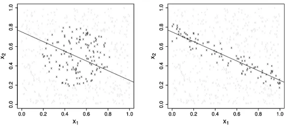
to an important bias. To illustrate this fact, letB0= (1,2)>/
√
thatS(B0)is a TDR subspace and that one is interested in the estimation of a conditional extreme
quantile ofY givenX =x0for a random vectorX = (X(1), X(2))>withX(1)andX(2)independent
and uniformly distributed on(0,1). In this situation, the points of interest are those located on the
set{x= (x(1), x(2)); B0>x=B0>x0}. On Figure 1, observations amongn= 500independent copies
X1, . . . , Xn ofX for whichK(hn−1B0>(x0−Xi))>0(left panel) andK(Mn−1(x0−Xi))>0(right
panel) are represented forhn = 1/10. It clearly appears that the observations used to compute
ˇ
Qn(·|B0, x)(right panel) are more relevant than the ones used inQˇn(·|x)(left panel).
3.2
Conditional extreme quantile estimation: the case
B
0unknown
First, a procedure to estimate the subspace S(B0) (i.e. the matrix B0) is proposed. In what
follows, it is assumed thatsupp(X) =Rp. In this case, we have the following result.
Proposition 3. If supp(X) =Rp then a minimum TDR subspace is unique.
The starting point for the estimation ofB0is a result showing thatB0can be seen as the solution
of a minimization problem. Let us first introduce some notation. ForJ ∈N∗ and for any matrix
B ∈ B, let {Πj(B>X), j = 1, . . . , J} be a random partition of supp(X). In the sequel, it is
assumed that for allB ∈ B and allj= 1, . . . , J,P(X ∈Πj(B>X)|B>X)>0 a.s. (an example of
such a partition is given in Section 4). Let us also introduce the functionT : (0,1)× B 7→[0,∞]
defined by T(α, B) := J X j=1 E P({Y > Q(α|B>X)} ∩ {X ∈Πj(B>X)}|B>X) αP(X∈Πj(B>X)|B>X) −1 2 .
According to the second statement of Theorem 1, the quantity T(α, B0) is close to 0 for small
values ofα. This argument suggests that an approximation ofB0 can be obtained by minimizing
the functionT(α, B)withαsmall. More precisely, introducing the notation
˜
B0(α) := arg min
B∈B
T(α, B), (14)
we have the following result.
Theorem 3. Assume that there exists a full rank matrix B0 ∈ B such that S(B0) is a
mini-mum TDR subspace and that supp(X) =Rp. If for all κ >0 and ε >0, there exists α0 ∈(0,1)
such that for allα∈(0, α0),P[δα(B>0X)< κ] = 1and
sup B∈B min ( P(Y > Q(α|B>X)|X) α −1 ; P(Y > Q(α|B>X)|X) α −1 −1) −L˜(B) ≤ε, (15)
for some functionL˜(·) :B 7→[0,∞)then kB˜0(α)−B0k →0 asα→ 0 wherek · k is any matrix
norm.
The condition on the random variableδα(BT
0X)(which was defined in (11)) entails thatQ(α|B0>X =
B>
0x) converges to the endpoint Q(0|B0>X =B0>x) uniformly on x∈ supp(X) as α goes to 0.
Condition (15) ensures that, uniformly onB∈ B,|α−1
P(Y > Q(α|B>X)|X)−1|admits a positive
(possibly infinite) limit asαgoes to 0.
As a conclusion, Proposition 3 and Theorem 3 ensure that the solution of the minimization
prob-lem (14) converges to the unique directionB0 as α→0. This naturally motivates us to estimate
similar procedure was used by Ichimura [25] to estimate the direction of a single-index model.
To construct this estimator, let us introduce a sequence(αn)converging to 0 with the sample size.
The sample analog ofT(αn, B)is given by:
1 n2 J X j=1 ( n X i=1 Φn,j(B>Xi) αnpj(B>Xi) −1 )2 , (16)
with forB∈ B,z∈supp(B>X)andj∈ {1, . . . , J},pj(z) :=P(X ∈Πj(B>X)|B>X =z)fB>X(z)
(wherefB>X(·)is the probability density function of B>X) and
Φn,j(z)
fB>X(z)
:=P {Y > Q(α|B>X =z)} ∩ {X ∈Πj(B>X)}|B>X =z.
Obviously, in practice, random variablesΦn,j(B>Xi)andpj(B>Xi)are not observed and must be
replaced by their respective kernel estimators: b Φn,j(B>Xi) :=X `6=i I{Y`>Qbn,−i(αn|B>Xi)}I{X`∈Πj(B>Xi)}K(H −1 n B >(X i−X`)),
whereQbn,−i(αn|B>Xi)is the conditional quantile estimator defined in (4) computed without the
couple(Xi, Yi)and b pj(B>Xi) := X `6=i I{X`∈Πj(B>Xi)}K H −1 n B>(Xi−X`) .
We can now introduce our estimator ofB0:
b
B0,n=Bb0,n(Hn, αn) := arg min B∈B
b
Tn(B), (17)
whereTbn(B) is obtained by replacing in (16) the unobserved random variablesΦn,j(B>Xi)and
pj(B>Xi)byΦbn,j(B>Xi)andpbj(B
>X
i).
We can now propose a more useful estimator ofQ(βn|X =x)than the one obtained in Section 3.1.
Replacing B0 byBb0,n in (6) leads to the estimator Qˇn(βn|Bb0,n, x) than can be use in the more
realistic situation where the true directionB0is unknown.
The simulation study presented in Section 4 seems to prove that this estimation procedure does work in practice. The optimization problem (17) is solved by using a coordinate search method
(see Section 4.1 for more details). Note that whenq > 1, the computational cost of this solving
method is important. This is the reason why we focus only on the situationq= 1in the simulation
study.
Of course, one may wonder if the obtained statisticBb0,nis a good estimator (in some sense) ofB0.
To establish the theoretical consistency ofBb0,n, a possible way is to follow the lines of the proof
of [25, Theorem 5.1] where anM-estimator of the direction in a single-index model is proposed.
This proof requires the uniform consistency onB ∈ Bof the estimatorTbn(B)ofT(B)to be shown.
This is an interesting but non-trivial result that is beyond the scope of the present paper.
4
Simulation study
4.1
Estimation of the TDR subspace in practice
Let(X, Y)be a random vector and assume that there exists a full rank matrixB0 of rank q < p
of the random couple(X, Y), we present below a procedure to compute the estimator (17) of the
directionB0.
Construction of the partition− LetD= [d1, . . . , dp]be ap×porthogonal matrix such that
S(B)is spanned by{d1, . . . , dq}. The matrixD is obtained by using the Gram-Schmidt process.
Letm(B>x)be the conditional marginal median ofXgivenB>X =B>xand for`∈ {1, . . . , p−q},
let us introduce the half spaces
E`(B>x) :={s∈Rp; d>`+qs > d > `+qm(B >x)} and E¯`(B>x) :={s∈Rp; d>`+qs≤d > `+qm(B >x)}.
An element of the partition{Πj(B>X =B>x), j= 1, . . . , J}is the intersection ofp−qhalf spaces.
More specifically, an element of the partition is a setE1∗∩. . .∩Ep∗−q where for`∈ {1, . . . , p−q},
E∗` ∈ {E`(B>x),E¯`(B>x)}. There is thus J = 2p−q elements in the partition. Obviously, if
supp(X) =Rp, then, for allx∈Rpand, for allj∈ {1, . . . , J},P(X∈Πj(B>X)|B>X=B>x)>0.
In practice, since the conditional marginal median m(B>x) is unknown, it is replaced by its
empirical estimatormbn(B>x) := (mbn,j(B>x), j= 1, . . . , J)>where forj = 1, . . . , J,mbn,j(B>x)is
the empirical median of the j-th component of the observations falling inD(B>x, Hn). This choice
of random partition ensures that, for allx∈supp(X), the number of available observations in each
element ofD(B>x, Hn)∩Πj(B>X=B>x)is approximatively the same. For a better view of the
previously constructed partition, let us give an example. LetX= (X(1), X(2))>be a random vector
whereX(1)andX(2)are independent and uniformly distributed on[0,1]. In Figure 2, the partition
{Π1(B>X =B>x),Π2(B>X =B>x)}ofsupp(X) = [0,1]2is represented forB= (1,2)>/
√
5and
x = (3/5,1/5)>. Using n = 500 independent copies of X and taking Hn = 50/n = 0.1, the
conditional marginal medianm(B>x)is estimated bymbn(B>x) = (0.416,0.280)>.
Computation of Tbn(B) − The previously defined partition is used to compute the sample
analog (16) of T(αn, B) for any given matrix B. Using the whole sample {X1, . . . , Xn} is time
consuming since the partition must be computed for each observationsXi, i= 1, . . . , n. We thus
choose to use only a random subsample of sizen0:=bancfor a givena∈(0,1)to compute (16).
Extensive simulation studies show that this procedure does not affect too much the quality of the
obtained estimator ofB0 (see Section 4.3).
Minimization of the function Tbn(·) − To solve this optimization problem, we choose to use
the coordinate search method (see for instance [23]). Starting with a matrixB0∈ B, this method
tries to find a new matrixB1∈ Bsuch that the value of the objective function atB1is smaller than
the one atB0. The new matrixB1is obtained in the following way: we first compute a matrixBˇ1
by adding or subtracting the search distanceδto a single coordinate in each row ofB0. We then
compute the matrixB1∈ B such that span(B1) = span( ˇB1). If such a matrix can be found then
B0is replaced byB1, the search distanceδis increased and the previous procedure is repeated. If
not, the previous procedure is repeated with B0 and a smaller value ofδ. More specifically, the
coordinate search method used in this paper is described below:
•Initialization: TakeB(0) ∈ B,δ(0)>0 andδtol>0.
•Step k: let(e1, . . . , ep)be the canonical basis ofRp and, fori= 1, . . . ,2p, lete˜i := (−1)iedi/2e.
linearly independent columns of the projection matrix on the set spanned by the columns of the
matrixB(k−1)+δ(k−1)E˜ with E˜ = [˜ei1, . . . ,˜eiq]. Denoting by B
(k) the set of the (2p)q matrices
˜
B(i1,...,iq),(i1, . . . , iq)∈ {1, . . . ,2p}
q, there are two possibilities
−ifTbn(B(k−1))≤min{Tbn(B), B∈ B(k)}, then B(k)=B(k−1) andδ(k)=δ(k−1)/2, −ifTbn(B(k−1))>min{Tbn(B), B∈ B(k)}, then B(k)= arg min B∈B(k) b Tn(B)andδ(k)= 2δ(k−1).
•Ifδ(k)> δtol, go to stepk+ 1, else, the algorithm is stopped.
The next section is dedicated to the presentation of the models considered in the simulation study.
4.2
Model setting
In what follows, the pcomponents of the random vector X are independent and distributed as
a Gaussian random variable with mean1/2 and variance σ2. The dimension of the explanatory
variableX is fixed top= 4and the responseY is generated according to the following models: for
positive functionsg0(·),g1(·),g2(·), forB0∈R4 andB1∈R4, the conditional quantile ofY given
X=xis given forα∈(0,1)and x∈Rp by:
Model 1−Q1(α|X =x) := [ln(1/(1−α))]− g0(B0>x)1 +g 1(B1>x) exp(−α−1) −1 . Model 2−Q2(α|X =x) :=g2(B0>x)−[ln(1/(1−α))] g0(B0>x)1 +g 1(B1>x) exp(−α−1) . Model 3−Q3(α|X =x) := [ln(1/α)]g0(B > 0x)1 +g 1(B>1x) exp(−α−1) −1 .
Denoting by S1(y|x)(resp. S2(y|x), S3(y|x)) the conditional survival function P(Y > y|X =x)
when(X, Y)is distributed from Model 1 (resp. Model 2, Model 3), it is proved in Lemma 4 that
for allx∈Rp andδ >0
S1(δ−1|x) =δ1/g0(B > 0x)L 1(δ−1|x), S2(g2(B0>x)−δ|x) =S1(δ−1|x) and S3(δ−1|x) = exp h −δ−1/g0(B>0x)L 3(δ−1|x) i ,
whereL1(y|x)andL3(y|x)converge to 1 asy→ ∞.
The first statement of [22, Theorem 1.2.1] entails that S1(·|x) is in the maximum domain of
at-traction of Fréchet with positive extreme value index γ(x) = g0(B>0x) and, as a consequence,
condition (5) is satisfied byQ1(·|X =x).
According to the second statement of [22, Theorem 1.2.1], S2(·|x) is in the maximum domain of
attraction of Weibull with a negative extreme value indexγ(x) =−g0(B>0x)and a right endpoint
Q2(0|X =x) =g2(B0>x).
Finally, for all x ∈ Rp, S3(·|x) is a Weibull-tail distribution (see for instance [19] for a
defini-tion). As a consequence,S3(·|x)belongs to the Gumbel maximum domain of attraction and thus
Q3(·|X =x)satisfies (5) with an extreme value index equal to 0.
The following parameterization is considered in the sequel: g0(·) := ˜g(z; 1/3,8/3) and g2(·) :=
˜
g(z; 1,10)where fora < bandz∈R,
˜ g(z;a, b) =aI(−∞,0)(z) + a+b exp(2z)−1 exp(6/√5)−1 I[0,3/√5)(z) + (a+b)I[3/√5,∞)(z).
Note that for allz∈R,g˜(z;a, b)∈[a, a+b]. The functiong1(·)is defined byg1(z) =I(−∞,0)(z) +
exp(5z)I[0,2)(z) + exp(10)I[2,∞)(z). Finally,B>0 := (2,1,0,0)/
√
5and B1> := (0,0,1,1). It can be
shown (see Lemma 4, appendix A) that for all these models,S(B0)is a TDR subspace (withq= 1)
and that condition (9) is satisfied.
4.3
TDR subspace and conditional quantile estimation
For each model introduced in Section 4.2,N = 100samples of sizen= 4000 are generated. Our
purpose is to appreciate the finite sample performance of the TDR subspace estimator defined
in (17) and to compare three different estimators of the conditional extreme quantileQ(βn|X =x)
of orderβn = 2/n: (a) estimator Qˇn(βn|B0, x) for the (unrealistic) situation where the TDR
di-rection B0 is known, (b) the more useful plug-in estimator Qˇn(βn|Bb0,n, x) and (c) the classical
estimator Qˇn(βn|x) := ˇQn(βn|Ip, x) when the existence of a TDR subspace is not taken into
account.
TDR subspace estimator To compute the estimator, we takeαn=n−1/3,Hn=n−2/9 and a
subsample of sizen0= 100. Obviously, hidden parameters αn andHn have a strong influence on
the quality of the estimation. In the real data application, a procedure to choose these parameters
is proposed. In the simulation study, we decide to fix the values ofαn and Hn by eye in order to
focus only on the estimation of the TDR subspace. The influence of the subsample sizen0 is less
critical. To support this assertion, the estimation ofB0 has been considered under model 1 with
σ= 1/5forn0∈ {2,4, . . . ,20,25,50,75,100,150,200,250,300}. In figure 3, the empirical quantiles
of order 0.05, 0.5 and 0.95 ofkBb0,n−B0kF (where for all matrix B,kBkF := [tr(B>B)]1/2 is the
Frobenius norm) are represented as a function of n0. It appears that for n0 > 75, the quality
of the estimation does not clearly depends onn0. Recall also that an initialization is required in
the coordinate search method used to compute the TDR subspace estimator. In this simulation
study, the initial vectorB(0)is randomly chosen. More specifically,B(0)= (u
1, . . . , up)/[u21+. . .+
u2p]1/2 where u1, . . . , up are realizations of pindependent random variables uniformly distributed
on[−1,1].
The estimatorBb0,n ofB0 is compared with the one obtained by the SIR method. Recall that the
SIR estimatorBb0SIR,n corresponds to theqeigenvectors associated to theqlargest eigenvalues of the
matrixΣb−n1bΓn with b Σn := 1 n n X i=1 Xi− 1 n n X i=1 Xi ! Xi− 1 n n X i=1 Xi !> andΓnb := J X j=1 nj n 1 nj X i:Yi∈Rj Xi− 1 n n X i=1 Xi 1 nj X i:Yi∈Rj Xi− 1 n n X i=1 Xi > ,
where {R1, . . . , RJ} are non-overlapping slices that cover the range of Y and nj is the number
of Yi’s lying in Rj. To compute the SIR estimator, the R package dr (see [36]) was used with the default method to construct the slices. The SIR method focus only on the central part of
the conditional distribution ofY givenX and is thus generally not adapted for the estimation of
the TDR subspace. The accuracy of the TDR direction estimators is measured by the Frobenius
Conditional quantile estimators Here also, since our purpose is to compare three different
estimators of the same quantity, it seems more adequate to fix the hyperparametersαn and Hn.
As before, we takeαn =n−1/3. For estimatorsQˇn(βn|B0, x)andQˇn(βn|Bb0,n, x), the bandwidth
is Hn = n−2/9. For Qˇn(βn|x), the p×p matrix Hn is given by [n−2/9]1/4I4. According to the
third remark after Theorem 2, this choice ensures that estimators Qˇn(βn|B0, x) and Qˇn(βn|x)
share the same rate of convergence. To compute the conditional tail index estimator (7) and the
auxiliary function estimator (8) we takeν = 0.02 and ϕ(·) = ln(1/·) (this choice was suggested
in [16]). Concerning the kernel functionK(·)we take the Epanechnikov kernel. It is well known
that in practice, the choice of the kernel function is not crucial (see for instance [10]). To assess the estimation procedure, we compute for each replication the error
EQ( ˇB) := 1 card(L) X x∈L ln Qˇ(βn|B, xˇ ) Q(βn|X =x) 2 ,
whereL is the set{(x1, . . . , x4); xi∈ {1/4,1/2,3/4}fori= 1, . . . ,4} withcard(L) = 34= 81and
ˇ
B∈ {Bb0,n,Bb0SIR,n, Ip}.
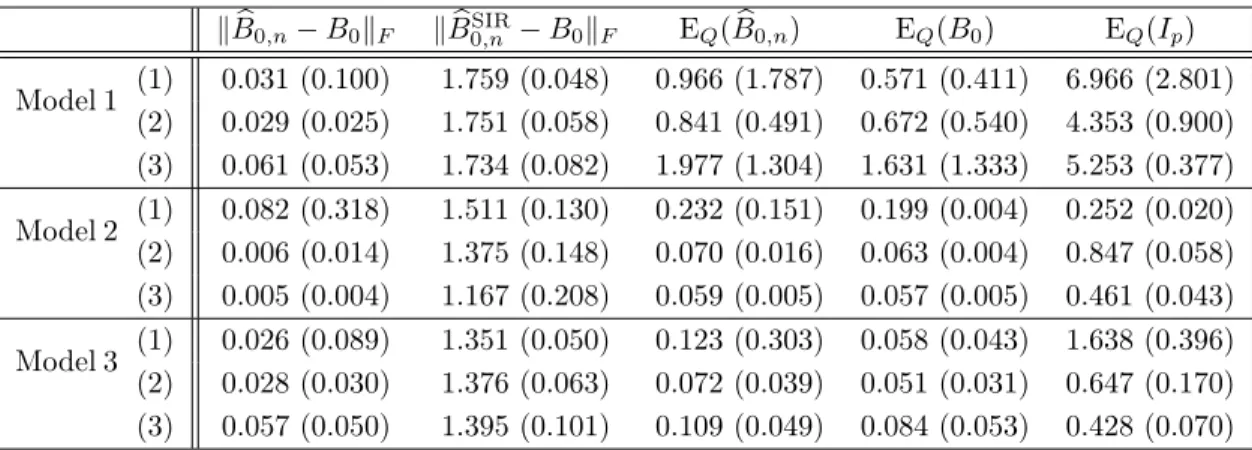
Results are gathered in Table 1. As expected, the conditional extreme quantile estimatorQˇn(βn|B0,·)
is the best among the three considered statistics. Unfortunately, this estimator can only be used
in the ideal situation whereB0 is known. Nevertheless, the plug-in estimatorQˇn(βn|Bˆ0,n,·)
pro-vides similar results and outperforms in each case the classical estimatorQˇn(βn|Ip,·)(for which
the existence of a TDR subspace is not assumed). One can remark that even for a large
sam-ple size (n= 4000), the classical estimator performs very poorly for a 4−dimensional covariate.
There is thus a real benefit in using our dimension reduction procedure. Note also that the
TDR estimatorBˆ0,n provides good estimation of the true directionB0while, as expected, the SIR
estimatorBˆSIR
0,n is not able to find the true direction. It appears in fact that Bˆ0SIR,n is often close
to the “central” directionB1 = (0,0,1,1)>. For instance, whenσ = 1/3, kBˆSIR0,n −B1kF = 0.016
for Model 1, kBˆSIR
0,n −B1kF = 0.066 for Model 2 and kBˆ0SIR,n −B1kF = 0.110 for Model 3. This
confirms the fact that classical dimension reduction methods are not adapted to the study of the
tail of the conditional distribution. Note also that the value of the standard deviationσ has an
influence on the estimation ofB0. Except for Model 2, the performance of Bˆ0,n deteriorates asσ
decreases. One possible explanation is that whenσis small, the variance ofγ˜(B>
0X)is also small is
thus the true direction is difficult to capture. Finally, to illustrate the sensitivity to the hidden
pa-rametersαn andHn, I estimate the TDR direction and the conditional quantile of orderβn = 2/n
under model 1 withσ = 1/8 and with the following hidden parameters: (1) αn = Hn =n−1/3,
(2) αn = n−1/3 and Hn = n−1/10 and (3) αn = Hn = n−1/10. Results are given in Table 2.
As expected, the conditional quantile estimator is sensitive to a bad choice of αn and Hn. The
estimator ofB0 seems to be more robust.
Choice of the TDR dimension In this simulation study, we assume that the true dimensionq
of the minimum TDR subspace is known. Obviously, in practice, this is not the case andqneed
to be estimated. In a non extreme-value context, some approaches for the estimation ofqcan be
found in the literature (see for instance [6] where a general permutation test is proposed and [5] for the use of information criterion). Adaptation of these methods to our situation is beyond the
scope of this paper. Nevertheless, in our setting, a possible way to check that the choiceq = 1
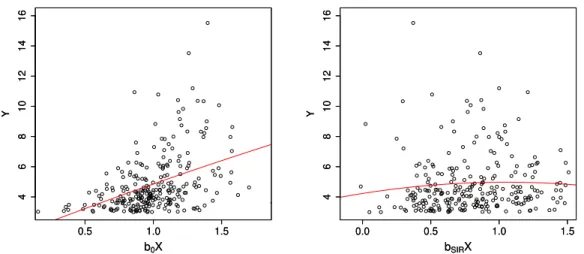
is reasonable is to look at the scatter plot of the largest observations{Yn−bnαc+1,n ≤. . .≤Yn,n}
statisticYn−i+1,n andBb0,n∈Rp is the estimated direction obtained in Section 4.1. The presence
of a relationship between extreme values ofY and their corresponding projections onBb0,n is a
good indicator that the projectionBb>0,nX contains most of the information on the tail
distribu-tion ofY. This scatter plot is represented on Figure 4 for a sample of size n = 4000 generated
according to Model 1 withσ= 1/3. As before,αn =n−1/3 and Hn =n−2/9. On the left panel,
the directionB0 is estimated by the procedure described in Section 4.1 while on the right panel,
this direction is estimated by the SIR approach. A strong link between extreme values ofY and
their corresponding projections can be seen on the left panel. In contrast, extreme values seem uniformly distributed on the right panel. This scatter plot is therefore a useful graphical tool that
permits us to visually check the relevance of a TDR model withq= 1. The right panel confirms
again that classical dimension reduction methods are not always useful when one is interested in the tail of the conditional distribution.
5
Data analysis
According to the world health organization, atmospheric pollutants may cause serious effects on public health and on environment. One of the most dangerous pollutant in urban areas is ozone. It is generated in the air when others pollutants (called primary pollutants) react with atmospheric oxygen and weather conditions (temperature, humidity, etc.).
Our objective is to understand the relationship existing between the concentration of some pri-mary pollutants and the daily maximum surface concentration of ozone. Our study is based on
data collected in Chicago from 1987 to 2000 duringn = 4841days. These data are available on
theRpackageNMMAPS Data Lite. The dataset consists in daily concentrations of different
pollu-tants such as ozone (O3), particular matter with diameter smaller than 10 microns or 25 microns
(PM10 or PM25), sulphur dioxide (SO2), nitrogen dioxide (NO2), carbon monoxide (CO), etc.
Various meteorology and mortality variables were also recorded. These data were considered by many authors in a dimension reduction framework (see for instance [33] and [38]).
More specifically, letY be the concentration of O3 (in parts per billion) and X be the covariate
vector of dimensionp= 4corresponding to the daily maximum concentrations of PM10, SO2, NO2
and CO. Note that for numerical convenience, the components ofX are centered and normalized.
We are interested in the estimation of extreme quantiles of orderβn = 1/nof the conditional
distri-bution ofY givenX=xwith two different possible scenarios forx. LetxPM10
τ ,xSOτ 2,xNOτ 2andxCOτ
be the empirical quantile of order1−τ ∈(0,1) of the (centered and normalized) daily maximum
values of PM10, SO2, NO2and CO. The first scenario isx= (xPM.5 10, x
SO2
.5 , x NO2
.5 , xCO.5 )>. This joint
vector is quite close to a situation observed in Chicago during the period 1987-2000 with moderate
values of the four primary pollutants. A second likely scenario isx= (xPM10
.5 , x SO2
.25 , x NO2
.05 , xCO.05)>
corresponding to large values for NO2and CO.
In a first step, we assume the existence of a TDR subspace forY givenX of dimensionq= 1. To
compute the TDR estimator proposed in this paper, we use the Epanechnikov kernel. A choice
for the bandwidth Hn, the percentage of largest observations αn and the sizen0 of the random
subsample is also required. As mentioned in Section 4.2, the choice ofn0is not critical and we fix it
is used. LetH:={0.05, . . . ,0.25} andA:={0.01, . . . ,0.1}be two sets of possible 10 equi-spaced
values forHn andαn. The selected values ofHn andαn are given by
ˆ Hn,αˆn := arg min (h,α)∈H×A b Tn b B0,n(h, α) .
The idea motivating this criteria is that for well chosenHnandαn, the value ofTbn
b
B0,n(Hn, αn)
must be close to 0. For the Chicago air pollution dataset, this procedure leads toˆhn= 0.094and
ˆ αn= 0.09(withTbn b B0,n(0.094,0.09)
= 0.006). The estimated direction is
b
B0,n= (0.175,−0.036,0.962,−0.207)
>
.
Note that the coordinate search method was initialized with different vectorsB(0), all these
ini-tialization leading to very similar values ofBb0,n.
In the first step, the existence of a TDR subspace of dimensionq = 1 was assumed. We must
now check if this assumption seems reasonable for the Chicago air pollution dataset. The
scat-ter plot introduced in Section 4.3 (Choice of the TDR dimension) is presented on Figure 5. A
pattern clearly appears in this plot. This is a first clue that the projection of X on Bˆ0,n
con-tains a non negligible amount of information on the tail distribution ofY. The scatter plot can
be completed by the value of the correlation between Y and Bˆ0>,nX. This correlation is equal
toCor(Y,Bˆ0>,nX) = 0.58 and has to be compared to correlations between Y and each individual
covariate: Cor(Y, P M10) = 0.37;Cor(Y, SO2) = 0.05;Cor(Y, N O2) = 0.55andCor(Y, CO) = 0.17.
It appears thatY is more correlated with the projection ofX onBˆ0,n than with each individual
covariate. We can also remark thatCor(Y, N O2)≈Cor(Y,Bˆ0>,nX) which is not surprising since
b
B0,nis close to the directionb0:= (0,0,1,0)> (kBˆ0,n−b0kF = 0.08). The covariate NO2seems to
bring the most important information on large values of ozone concentration.
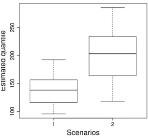
We can now proceed to the estimation of conditional extreme quantiles for the two considered scenarios. In order to have an information on the distribution of the conditional quantile esti-mator, a jackknife resampling method is used. More specifically, we first select the observations
corresponding to thebnαˆnc = 435largest values of Y. A sample distribution of the conditional
quantile estimator is then obtained by leaving out each selected observations and computing the estimator. For each scenario, we represent the box-plot of the jackknife distribution (see Figure 6). It appears that the worst scenario for large values of ozone concentration is the second one: very
important ozone concentration is more likely to be observed when concentrations of NO2 and CO
are important. Controlling levels of NO2and CO can thus lead to a reduction in ozone
concentra-tion. This conclusion is in line with the paper of Hanet al.[24] where it is shown that “the levels
of O3 and NO2are inextricably linked”.
Conclusion
We propose in this paper a new dimension reduction framework dedicated to the study of the
tail of a distribution in presence of a covariate of dimension p. An estimation procedure of the
reduced subspace and conditional extreme quantiles is presented. It appears on our simulation
study that even for a moderate dimensionp of the covariate (for instance p = 4), the classical
kernel estimator of conditional extreme quantiles fails to approximate the true quantile while our procedure provides significantly better results.
References
[1] Araújo Santos, P., Fraga Alves, M.I. and Gomes, M.I. (2006). Peaks Over Random Threshold
methodology for tail index and high quantile estimation, REVSTAT,4(3), 227–247.
[2] Basu, D. and Pereira, C.A.B. (1983). Conditional independence in statistics,Sankhya,45(3),
Series A, 324–337.
[3] Chaudhuri, P. (1991). Nonparametric estimates of regression quantiles and their local Bahadur
representation,Annals of Statistics,19(2), 760–777.
[4] Cook, R.D. (1994). On the interpretation of regression plots,Journal of the American
Statis-tical Association,89(425), 177–189.
[5] Cook, R.D. and Forzani, L. (2009). Likelihood-based sufficient dimension reduction, Journal
of the American Statistical Association,104, 197–208.
[6] Cook, R.D. and Weisberg, S. (1991). Discussion of "Sliced Inverse Regression for dimension
reduction",Journal of the American Statistical Association,86, 328–332.
[7] Daouia, A., Gardes, L. and Girard, S. (2013). On kernel smoothing for extremal quantile
regression, Bernoulli,19(5B), 2557–2589.
[8] Daouia, A., Gardes, L., Girard, S. and Lekina, A. (2011). Kernel estimators of extreme level
curves,Test,20(2), 311–333.
[9] Davison, A.C. and Smith, R.L. (1990). Models for exceedances over high thresholds,Journal
of the Royal Statistical Society, series B,52, 393–442.
[10] Davison, A.C. and Ramesh, N.I. (2000). Local likelihood smoothing of sample extremes,
Jour-nal of the Royal Statistical Society, series B,62, 191–208.
[11] Dekkers, A. L. M., Einmahl, J. H. J. and de Haan, L. (1989). A moment estimator for the
index of an extreme-value distribution,The Annals of Statistics,17(4), 1833–1855.
[12] Eastoe, E.F. and Tawn, J.A. (2009). Modelling non-stationary extremes with application to
surface level ozone,Journal of the Royal Statistical Society, series C,58, 25–45.
[13] Fisher, R. A. and Tippett, L. H. C. (1928). Limiting forms of the frequency distribution of the
largest or smallest member of a sample, Proceedings of the Cambridge Philosophical Society,
24, 180–190.
[14] Fraga Alves, M. I., Gomes, M. I., de Haan, L. and Neves, C. (2007). A note on second order
conditions in extreme value theory: linking general and heavy tail conditions, REVSTAT
-Statistical Journal,5(3), 285–304.
[15] Gannoun, A., Girard, S., Guinot, C. and Saracco, J. (2004). Sliced inverse regression in
reference curves estimation,Computational Statistics and Data Analysis,46(1), 103–122.
[16] Gardes, L. (2015). A general estimator for the extreme value index: applications to conditional
and heteroscedastic extremes,Extremes,18(3), 479–510.
[17] Gardes, L. and Girard, S. (2010). Conditional extremes from heavy-tailed distributions: an
[18] Gardes, L. and Girard, S. (2012). Functional kernel estimators of large conditional quantiles,
Electronic Journal of Statistics,6, 1715–1744.
[19] Gardes, L. and Girard, S. (2016). On the estimation of the functional Weibull tail-coefficient,
Journal of Multivariate Analysis, 146, 29–45
[20] Gasser, T. and Müller, H.G. (1984). Estimating regression functions and their derivatives by
the kernel method, Scandinavian Journal of Statistics,11, 171–185.
[21] Gnedenko, B. V. (1943). Sur la distribution limite du terme maximum d’une série aléatoire,
Annals of Mathematics,44, 423–453.
[22] de Haan, L. and Ferreira, A. (2006).Extreme Value Theory: An Introduction, Springer.
[23] Hooke, R. and Jeeves, T.A. (1961). Direct search solution of numerical and statistical
prob-lems,Journal of the ACM,8(2), 212–229.
[24] Han, S., Bian, H., Feng, Y., Liu, A., Li, ., Zeng, F. and Zhang, X. (2011). Analysis of the
relationship between O3, NO and NO2 in Tianjin, China,Aerosol and Air Quality Research,
11, 128–139.
[25] Ichimura, H. (1993). Semiparametric least squares (SLS) and weighted SLS estimation of
single-index models, Journal of econometrics,58, 71–120.
[26] Koenker, R. and Basset, G.S. (1978). Regression quantiles,Econometrica,46, 33–50.
[27] Li, K.C. (1991). Sliced inverse regression for dimension reduction.Journal of the American
Statistical Association,86, 316–327.
[28] Li, K.C. (1992). On principal hessian directions for data visualization and dimension reduction:
another application of Stein’s lemma, Journal of the American Statistical Association, 87,
1025–1039.
[29] Nadaraya, E.A. (1964). On estimating regression, Theory of Probability and its Application,
9(1), 141–142.
[30] Northrop, P.J. and Jonathan, P. (2011). Threshold modelling of spatially dependent
non-stationary extremes with application to hurricane-induced wave heights, Environmetrics,
22(7), 799–809.
[31] Parzen, E. (1962). On the estimation of a probability density function and mode,Annals of
Mathematical Statistics,33, 1065–1076.
[32] Russell, B.T., Cooley, D., Porter, W.C., Reich, B.J. and Heald C.L. (2016). Data mining for
extreme behavior with application to ground level ozone, Annals of Applied Statistics, 10,
1673–1698.
[33] Scrucca, L. (2011). Model-based SIR for dimension reduction,Computational Statistics and
Data Analysis,55, 3010–3026.
[34] Wang, E. and Tsai, C. (2009). Tail Index Regression, Journal of the American Statistical
[35] Watson, G. S. (1964). Smooth regression analysis,Sankhya,26(15), 175–184.
[36] Weisberg, W. (2002). Dimension reduction regression inR,Journal of Statistical Software, 7,
1–22.
[37] Wu, T.Z., Yu, K. and Yu, Y. (2010). Single-index quantile regression,Journal of Multivariate
Analysis,101, 1607–1621.
[38] Xia, Y. (2009). Model checking in regression via dimension reduction, Biometrika, 96(1),
133–148.
[39] Yu, K. and Jones, M.C. (1998). Local Linear Quantile Regression,Journal of the American
Statistical Association,93(441), 228–237.
Appendix
−
Proofs
Preliminary results
The first Lemma is a probability result that will be helpful in the proof Theorem 1.
Lemma 1. Let (Ω,F,P)be a probability space. Let U be a positive random variable and V be a
Rq-valued random vector (U andV are both defined on(Ω,F,P)). Denoting byσ(U)(resp. σ(V))
theσ-algebra generated byU (resp. V), it is assumed thatσ(V)⊂σ(U). If there existsθ≥1 such that for allF ∈σ(U),
Z F E(U|V)dP≤θ Z F U dP or Z F E(U|V)dP≥θ−1 Z F U dP , (18)
thenE(U|V)≤θU a.s. (orE(U|V)≥θ−1U a.s.).
Proof−Assume that for allF ∈σ(U)
Z F E(U|V)dP≤θ Z F U dP,
(the proof for the other case is similar). First, we suppose thatUis a positive simple function. More
specifically, let{A1, . . . , Ak}be kdisjoint elements ofF with0<P(Ai)<1for alli∈ {1, . . . , k}.
We assume that U= k X i=1 ciIAi+ck+1I(A1∪...∪Ak)C,
where for all A ⊂ Ω, AC is the complement of A in Ω and c
i > 0 for all i ∈ {1, . . . , k}. Since
σ(V) ⊂σ(U), one can assume without loss of generality that σ(V) =σ({A1, . . . , A`}) with 1 ≤
` < k(the situation where`=k, i.e. σ(U) =σ(V)is trivial). It is then easy to check that
E(U|V) = ` X i=1 ciIAi+ξI(A1∪...∪A`)C, where ξ:= k X i=`+1 ci P (Ai) P[(A1∪. . .∪A`)C] +ck+1P [(A1∪. . .∪Ak)C] P[(A1∪. . .∪A`)C] .
We thus have to show that for everyi∈ {`+ 1, . . . , k},ξ≤θciand that, ifP[(A1∪. . .∪Ak)C]6= 0,
ξ≤θck+1. From (18), for allF ∈σ(U) =σ({A1, . . . , Ak}),
` X i=1 ciP(Ai∩F) +ξP[(A1∪. . .∪A`)C∩F]≤θ k X i=1 ciP(Ai∩F) +ck+1P[(A1∪. . .∪Ak)C∩F].
Forj ∈ {`+ 1, . . . , k}, taking F =Aj in the previous inequality leads toξ≤θcj sinceP(Aj)>0.
Furthermore, takingF= (A1∪. . .∪Ak)Centails thatξP[(A1∪. . .∪Ak)C]≤θP[(A1∪. . .∪Ak)C].
The result is thus proved for all positive simple functions. Since any positive measurable function is the pointwise limit of an increasing sequence of positive simple function, we conclude the proof by using the Lebesgue’s monotone convergence theorem.
The next lemma is a technical result used in the proof of Theorem 4.
Lemma 2. Assume that there exists a full rankp×qmatrixB0such thatS(B0)is a TDR subspace
forY given X and that condition (5) holds. For x∈ supp(X), let(yn(u|x))be a sequence such
that[yn(u|x)−Q(uαn|X =x)]/a(α−n1|X =x)→0 locally uniformly on u∈(0,∞). The following
statements hold almost everywhere forx∈supp(X):
(i) Let ν ∈ (0,1). For all u ∈ [ν,1], yn(u|x) =Q(β|B>0X = B0>x) with β ∈ [ξναn, ξ−1αn] for
ξ <1as near as you like to 1.
(ii) Let u ∈ (0,1) and ξ < 1 as near as we like to 1. If Q(0|X = x) < ∞ then Q(0|X =
x)−yn(u|x)≤ξ−1δαn(X =x)and if Q(0|X =x) = +∞ then[yn(u|x)]
−1≤ξ−1δ
αn(X =x).
Proof − We start by proving the first statement. From (5), one has for x ∈ supp(X) that
[yn(u|x)−Q(αn|X =x)]/a(α−n1|X =x)−Lγ(x)(1/u)→0 locally uniformly onu∈(0,∞). Now,
sinceS(B0) is a TDR subspace, [22, Lemma 1.2.12] entails that[Q(αn|X =x)−Q(αn|B>0X =
B0>x)]/a(α−n1|X =x)converges to 0 almost everywhere forx∈supp(X). As a first conclusion,
yn(u|x) =Q(αn|B0>X=B > 0x) +a(α −1 n |x) Lγ(x)(1/u) +o(1) ,
locally uniformly on u ∈ (0,∞) and almost everywhere for x ∈ supp(X). From Lemma 1, the
distribution function ofY givenB>0Xbelongs to a maximum domain of attraction with an auxiliary
function equivalent toa(·|x). Thus, according to [22, Theorem 1.1.6], one can findξ <1 as close
as we like to 1 such that for allu∈[ν,1], P(Y > yn(u|x)|B0>X =B0>x)≥νξαn. Hence,
yn(u|x) =Q P(Y > yn(u|x)|B0>X =B0>x))|B>0X=B0>x
≤Q(νξαn|B0>X=B0>x). (19)
Mimicking the proof of (19), we show thatyn(u|x)≥Q(ξ−1α
n|B0>X =B0>x)and thus conclude
the proof of the first statement.
Let us now focus on the second statement. Assume first thatQ(0|X =x)<∞ (this implies
that γ(x)≤0). Using the first statement withB0 =Ip, one has for all u≤1 and forξ˜as near
as we like to 1 that Q(0|X = x)−yn(u|x) ≤ Q(0|X = x)−Q( ˜ξ−1αn|X = x). Now from [22,
Lemma 1.2.9], one has that δ−αn1(X = x)a(α
−1
n |X = x) → −γ(x) as n goes to infinity. Hence,
from (5), one can findξ <1as near as we want to 1 such that
Q(0|X =x)−yn(u|x) δαn(X =x) ≤1 +Q(αn|X=x)−Q( ˜ξ −1α n|X =x) δαn(X =x) ≤ξ−1.
Now, suppose thatQ(0|X=x) = +∞(and thus thatγ(x)≥0). Applying again the first statement
want to 1. Sinceδαn(X =x)a(α
−1
n |X =x) =a(α−n1|X =x)/Q(αn|X =x)→γ(x)as n goes to
infinity, condition (5) entails thatδαn(X =x)Q( ˜ξ
−1α
n|X =x) = 1 +δαn(X =x)[Q( ˜ξ
−1α
n|X =
x)−Q(αn|X=x)]→ξ˜γ(x). Hence, one can findξ <1as close as we want to 1 and such that for
nlarge enough, yn(u|x)≥ξδα−n1(X =x)and the proof is complete.
Proofs of main results
Proof of Theorem 1−First, we prove that (i)implies(ii). Letε >0. There exists κ >0 such
that for allδ∈(0, κ],
∆δ(X, Z) := P(Y >Yδ(Z)|X, Z) P(Y >Yδ(Z)|Z) −1 ≤ε.
Remarking that for all non-zero bounded and positive functionh(·),
E I{Y >Yδ(Z)}h(X)|Z =Eh(X)E(I{Y >Yδ(Z)}|X, Z) Z .
it is easy to check that, almost surely, E(I{Y >Yδ(Z)}h(X)|Z) P(Y >Yδ(Z)|Z)E(h(X)|Z)−1 ≤E P(Y >Yδ(Z)|X, Z) P(Y >Yδ(Z)|Z) −1 h(X) E(h(X)|Z)|Z ≤ε. (20)
Let us now show that(ii)implies(i). We thus assume that for allε >0, there existκ > 0 such
that for allδ∈(0, κ], inequality (20) holds. LetA∈ B(Rp)andB ∈ B(Rq), we have
Z {X∈A}∩{Z∈B} P(Y >Yδ(Z)|Z)dP=EEI{X∈A}E(I{Y >Yδ(Z)}I{Z∈B}|Z)|Z = Z {Z∈B}P (Y >Yδ(Z)|Z)P(X ∈A|Z)dP = Z {Z∈B} P[{Y >Yδ(Z)} ∩ {X∈A}|Z] P(X ∈A|Z)P(X ∈A|Z) P[{Y >Yδ(Z)} ∩ {X ∈A}|Z] dP.
Letε∈(0,1). Applying inequality (20) withh(X) =IA(X)leads to Z {X∈A}∩{Z∈B} P(Y >Yδ(Z)|Z)dP≤ 1 1−ε Z {Z∈B} P[{Y >Yδ(Z)} ∩ {X∈A}|Z]dP and Z {X∈A}∩{Z∈B} P(Y >Yδ(Z)|Z)dP≥ 1 1 +ε Z {Z∈B} P[{Y >Yδ(Z)} ∩ {X ∈A}|Z]dP. Since Z {Z∈B} P[{Y >Yδ(Z)} ∩ {X ∈A}|Z]dP= Z {X∈A}∩{Z∈B} P(Y >Yδ(Z)|X, Z)dP,
and by the monotone class theorem we thus have for allF ∈σ(X, Z)that
1 1 +ε Z F P(Y >Yδ(Z)|X, Z)dP≤ Z F P(Y >Yδ(Z)|Z)dP≤ 1 1−ε Z F P(Y >Yδ(Z)|X, Z)dP.
We conclude the proof by applying Lemma 1 withU :=P(Y >Yδ(Z)|X, Z)andV =Z.
Let us now prove that(i) is equivalent to (iii). Obviously, if (i)holds then(iii)also holds with
To show that(iii)implies (i), first remark that the “tower property” of conditional expectations
entails thatP(Y >Yδ(Z)|Z) =E[P(Y >Yδ(Z)|X, Z)|Z] =sδ(Z)[1 +E(ηδ(X, Z)|Z)]a.s. Hence
P(Y >Yδ(Z)|X, Z) P(Y >Yδ(Z)|Z)
= 1 +ηδ(X, Z) 1 +E(ηδ(X, Z)|Z)
a.s. (21)
By assumption, for allε∈(0,1), there existsκ >0 such that for allδ∈(0, κ],
P P(Y >Yδ(Z)|X, Z) P(Y >Yδ(Z)|Z) −1 ≤ 2ε 1−ε = 1, (22)
which concludes the proof.
Proof of Proposition 1−First recall that sinceS(B0)is a TDR subspace, there exists a Borel
set A ∈ B(Rp)with
P(X ∈ A) = 1 such that for all x∈ A, Q(0|X = x) = Q(0|B0>X = B0>x).
Hence, for allx∈ A, [22, Lemma 1.2.12] and the definition of the TDR subspace entail that the
distribution functionP(Y ≤ ·|B>0X =B0>x)belongs to the maximum domain of attraction of an
extreme value distribution with extreme value indexγ(x) or equivalently that for all u >0 and
x∈ A
lim α→0
Q(uα|B0>X =B0>x)−Q(α|B0>X =B>0x)
a(α−1|x) =Lγ(x)(1/u). (23)
As a consequence, from [22, Theorem 1.2.6],for all x∈ A there exist positive functions c(·|B0>x)
andd(·|B0>x)(depending onxonly throughB0>x) such that for ally∈(y0, Q(0|B0>X =B0>x)),
P(Y > y|B>0X =B > 0x) =c(y|B > 0x) exp − Z y y0 ds d(s|B>0x) ,
with c(y|B>0x) → c0 > 0 as y → Q(0|B>0X = B0>x). Now, let us introduce the