Neural Voting Machines

Neural Voting Machines

Whitman Richards & H. Sebastian Seung

AI Memo 2004-029 December 2004

30 Dec 04

Neural Voting Machines

Whitman Richards & H. Sebastian Seung {wrichards,seung}@mit.edu

CSAIL

MIT 32-364, Cambridge, MA 02139

Abstract

“Winner-take-all” networks typically pick as winners that alternative with the largest excitatory input. This choice is far from optimal when there is uncertainty in the strength of the inputs, and when information is available about how alternatives may be related. In the Social Choice community, many other procedures will yield more robust winners. The Borda Count and the pair-wise Condorcet tally are

among the most favored. Their implementations are simple modifications of classical recurrent networks.

1.0 Introduction

Information aggregation in neural networks is a form of collective decision-making. The winner-take-all procedure is probably the most favored method of picking one of many choices among a landscape of alternatives (Amari & Arbib, 1977; Maas, 2000.) In the social sciences, this is equivalent to choosing the plurality winner, which is but one of a host of procedures that could be used to choose winners from a set of alternatives. More importantly, in the presence of uncertainty about choices, the plurality winner is not the maximum likelihood choice (Young, 1995.) To obtain a glimpse into some of the problems associated with winner-take-all, consider the analogy where the input is a population of voters. Then the plurality winner - that outcome shared by most of the voters -- only needs to receive more votes than any other alternative in the choice set. Hence it is possible for the winner to garner only a very small percentage of the total votes cast. In this case,

uncertainty and errors in opinions can have a significant impact on outcomes, such as when only a few “on-the-fence” voters switch choices. We sketch two other procedures that yield more reliable and robust winners. These procedures utilize information about relationships among alternatives, and can be implemented as neural networks.

2.0 Plurality Voting

To provide background, the winner-take-all procedure is recast as a simple voting machine. Let there be n alternative choices ai with vi of the voters preferring

alternative ai. The inputs to the n nodes in a neural network will then be the number

plurality_winner = argMax(i) {vi} [1]

which can be found using a recurrent network whose dynamics is described elsewhere (Xie, Hahnloser & Seung, 2001.) Note that no information about any similarity relationships among alternatives is captured in [1]. In other words, the Plurality voting method does not consider second ranked preferences of the voters.

3.0 Borda Method

To improve the robustness of outcomes, we now follow recommendations in Social Decision-Making, and relax the constraint that only first choices will be considered in the voting process (Runkel, 1956; Saari & Haunsberger, 1991; Saari, 1998.) Specifically, we include second (or higher) rank opinions, weighting these inversely to their rank when the tally is taken (Borda, 1784.) The minimum of these weighted sums is then taken as the winner. Here, we use the reversed Borda method, with the first choice given a weight equal to the largest rank, the weight on the

second choice being the next largest rank, etc. The winner is then the maximum of these weighted sums. To further simplify the computation and the network design, we assume the alternative choices are related by a model Mn that is held in common by

all voters. Each voter’s ranking of alternatives is now not arbitrary, but is also reflecting information about choice relationships (Richards et al, 1998, 2002.) Note that the effective role of Mn is to place conditional priors on the choice domain.

Although the shared model Mn has typically been represented as a graph, Gn,

it is more convenient to use the matrix Mij where the entry “1” indicates the

presence of the edge ij in Gn and 0 otherwise (Harary,1969). For the graphical

model of Fig 1, we would have:

0 1 1 0 0 1 0 1 0 0

Mij = 1 1 0 1 0 [2]

0 0 1 0 1 0 0 0 1 0

Here, for simplicity, we assume that the edges of Mn are undirected, meaning that if

alternative a1 is similar to alternative a2, then a2 is equally similar to a1. However,

directed edges require only a trivial modification to the scheme.

With Mn expressed as the matrix Mij we can include second choice opinions

in a tally by defining a new voting weight v*

i as

v*

i = { 2 vi + SjMij vj } [3]

where now first-choice preferences are given twice the weight of the second-ranked choices, and third or higher ranked options have zero weight. (This is the reverse Borda procedure.) The outcome is then

winner_Borda = argMax(i) {v*

i} [4]

A neural network that executes this tally is shown in Fig 1, and is a standard winner-take-all (WTA) network supplemented by an input layer. (The collection of WTA nodes in the “winner’s circle” does not show all the recurrent connections.) The ith WTA node receives a synapse of strength 2 from the ith input node, which in turn is driven by v_i. This twice weighted input to a WTA node is depicted by heavy double arrows. The ith WTA node also receives synapses of strength M_ij

from the jth input. These inputs are depicted by the slimmer arrows, each of which represents the assertion of an edge in M_n. In the neural network, one possible

implementation of these assertions would be a layer of neurons that inhibit inputs from v_i to v_j in the winner’s circle if edge [v_i,v_j] is not in M_n. The highlighted WTA node 3 is the Borda winner for the inputs v_i given in the model M_n. Note that the more common winner-take-all plurality procedure would pick node 1.

4.0 Bias Vector

A disadvantage of the Borda Count is that a weighting on preferences is imposed depending on rank. In our simple model using only first and second choice preferences, the weightings were 2 for the first choice and 1 for the second. Let this bias be represented as the vector {2, 1, 0}, where the 0 is the weight applied to all preferences ranked after second choices. Then it is clear that the bias for the

Plurality method is {1, 0, 0}. But we could also invent another bias vector {1, 1, 0} that would weight the “Top Two” choices equally. More generally, a normalized bias vector will have the form {1, b, c} with 0 < b < 1 and c = 0 for our simplified preference rankings. But now we see that the outcome of a Borda procedure will depend on the choices for b, c.

To avoid specifying values for b and c, alternatives can be compared pairwise. Each agent then simply picks the most preferred alternative of each pair – the one with the higher rank in his preference order. This method, proposed by Condorcet (1785) is a tournament, where the winner is that alternative beating all others. Definition: let dij be the minimum number of edge steps between vertices i and j in

Mn, where each vertex corresponds to the alternatives ai and aj respectively.

Then a pairwise Condorcet score Sij between alternatives ai and aj is given by

S_ij = S_k v_k sgn[ d_jk - d_ik] [5] with the sign positive for the alternative ai or aj closer to ak. Note that if ai or aj are

equidistant from ak, then sgn=0 and the voting weight vk does not contribute to Sij.

Furthermore, as in the Borda Count, we again impose a maximum on the value of dij of 2, which means that third or higher ranked alternatives do not enter into the

tally.

A Condorcet winner is then

winner_ Condorcet = ForAll_i=!=j Sij > 0 . [6]

Although a Condorcet winner is a true majority outcome, it comes at a

computational cost. For n alternatives, a complete pair-wise comparison would require

nC2or O(n

2_{) separate tallies. Hence a neural network that calculates the Condorcet}

5.0 Condorcet Network

To reduce the computational complexity to O(n), the trick is to choose a special subgraph of Gn, namely gk, with k << n. Conceptually, the subgraph we

choose is a ridge in the landscape of Borda weights. The ridge consists of the k nodes in Gn with the highest Borda scores. This choice is based on the observation

that for connected random graphs with weights chosen from a uniform distribution, there is a 90% likelihood that the Condorcet winner and the Borda winner will agree.

5.1 Specifics for the subgraph gk.

Let the Borda rank vector be {2,1,0} as before, with the Borda scores v*

i for

each vertex i in Gn. Without loss of generality, label the vertices in Gn by the rank

order of their Borda score, with vertex i = 1 having the largest score. In cases where the Borda scores are tied, simply choose the indexing arbitrarily among the tied vertices to create a total order. (If necessary, when ties occur for the kth and k+1 vertices, the size of gk may be increased to include all vertices with scores

identical to the kth ranked score.)

Definition: gk is the spanning subgraph of Gn containing the vertices with the top k

Borda scores.

Note that other definitions are possible. For example, we could require that gk be a

connected subgraph. In this case, for some Gn, gk may not include all the top k

Borda scores. Or, rather than ordering vertices using their Borda scores, the Top-Two bias vector {1, 1, 0} could be used. This latter choice may be more appropriate for scale-free graphs or trees with long paths between large clusters. The principal advantages of our definition are (i) ease of computation and (ii) uniqueness.

5.2 Sketch of a Neural Network

Here, our objective is to obtain a crude sense of the complexity of a plausible neural network that calculates a winner for gk. There are three design challenges:

(1) finding gk, (2) computing the Condorcet winner for each pairwise comparison,

and (3) to determine which alternative (node) beats all others. We assume that the maximum Borda ridge (nodes in gk ) has already been found. If gk can be

unconnected as defined, then a clipping algorithm might suffice. Alternatively, if we wish to impose a connectivity constraint on gk, then some form of a greedy

algorithm beginning at vertex i = 1 seems appropriate. Simulations based on random graphs Gn,for n=40 with edge probability 1/4 and weights chosen from a

uniform distribution show that in over 96% of cases, the winners with k=8 are the same regardless whether the definition of gk is satisfied precisely, or found using a

highest Borda scores will typically have the largest vertex degrees and hence the greatest connectivity. In either case, this step is of complexity O(n).

The second challenge is to implement kC2 pairwise comparisons [Eq. 5]. The

trick requires noting whether the vertices being compared are adjacent or not. Consider first the case where two vertices in gk are not adjacent in Gn (and hence

also not adjacent in gk.) Then we simply need to sum the weights of the neighbors

to each vertex, plus the weight of the vertex itself, and then compare these two weight sums to determine the pairwise winner. Note that this is equivalent to using the Top-Two bias vector {1,1,0} for each vertex, and then picking that vertex with the largest score. If the two vertices being contested are adjacent, however, then note that the weight of each vertex will be added to the score of the competing vertex. Hence the weights of the vertices themselves will be cancelled if the Top-Two bias vector is used. The patch is simple: just double the weight of each vertex when adjacent vertices are being contested. This is the Borda bias vector {2,1,0}. Hence, when calculating each pairwise Condorcet score, the rule is to use a Top-Two bias vector {1,1,0} when vertices are non-adjacent in Gn,, and to use the Borda

bias vector {2,1,0} when adjacent (Richards et al, 2002.) This requires making explicit whether or not the kC2 edges in gk are adjacent or not in Gn.

The third challenge is to determine that node or vertex beating all others. As will be seen below, this can be handled easily by a logical AND of the WTA outputs from each pairwise comparison.

Fig. 2 depicts a gk network with six layers. The computation is carried out as

follows:

(i) the k-maximum Borda ridge (nodes in gk) is given, as well as the

neighborhood sums in Gn for each node in gk .

(ii) activate the kC2 set of nodes in an “edge assertion” layer to make explicit

which edges in Mn are present in Gn (as was done previously in the Borda

network.) Note that this activation controls inputs to both the neighborhood sums layer, as well as to nodes in the comparator layer.

(iii) for every node in gk, find the sum of the weight of vertex i and its

neighbors (neighborhood sums.) Again, this step is analogous to that used in the Borda network of Fig. 1, except at this stage the sum uses the “Top-Two” bias vector. The second input for the weight of vertex i itself will be added in step (iv) depending upon edge connectivity in Gn.

(iv) project the “Top-Two” activity of neighborhood node sums onto each member of a pair of nodes in the “comparator” layer that has the same vertex label. (v) project the weight of vertex i itself onto the appropriate member of all pairs in the comparator layer, but only if the two vertices in the comparator layer are adjacent in gk (as controlled by the edge assertion

activations in (ii).)

(vi) use a WTA procedure to select the winner of each pairwise comparison in the comparator layer, and send either a “0” (loser) or “1” (winner) signal into the appropriate node in the “winner’s circle”.

(vii) do a logical “AND” of the inputs to each of the k nodes in the winner’s circle. If there is a unique winner, then only one node will remain active. If there is no such unique winner, then there is either a tie or a top-cycle. (A top-cycle is when alternative ai beats aj which in turn beats ak, and then ak

beats the original alternative ai.)

Note that although there are only k nodes in the winner’s circle, in the comparator layer there will be a much larger set of roughly 2 x kC2 depending upon the tiling.

This comparator layer, and also the comparable edge assertion layer, are the critical components that govern the size of the network. If the diameter of Gn is very large,

the connectivities required become too distant. Some hint of this problem is given in Fig. 2 for k = 4. This depiction also makes clear that neither Gn nor gk appear

explicitly as graphs. Rather, the connectivity is represented by the filled nodes that indicate whether the vector {2, 1, 0} or {1, 1, 0} should be applied to the paired comparison in the comparator module. This representational form has the obvious benefit that weighted edges, i.e. correlations among alternatives, can be easily be incorporated by allowing analog, rather than binary inhibition by the “edge assertion” nodes in layer 3 (small circles.)

6.0 Success of gk

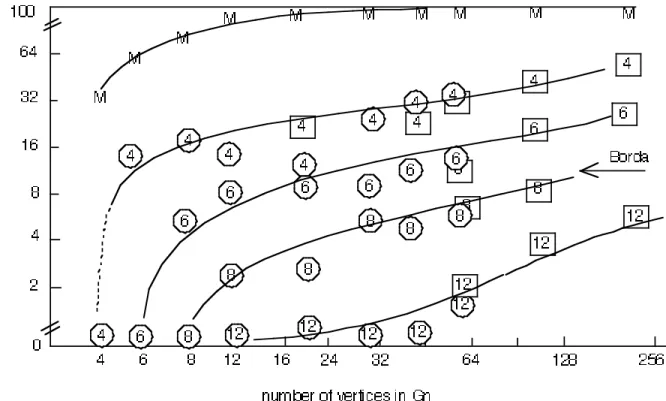
Figure 3 shows the success rate of the k-Condorcet procedure for graphs of size n < 250, with different choices for k. The models Mn used were connected

random graphs with edge probability 1/4. A set of weights on the nodes was chosen from a uniform distribution. Winners were also calculated using both the Plurality (i.e. node with greatest weight) and Borda procedures for the same set of weights. The graph shows the failure rate of gk to yield the same Condorcet winner

the Gn winner (98+% for k > 8.) The approximation by gk is thus conservative:

there are few false positives, instead no winner is chosen, unlike the Borda count.

!

Figure 4 provides some additional insight into the robustness of the several aggregation procedures. Here again, random graphs of edge probability 1/4 were generated, with weights on nodes chosen from a uniform distribution. Winners were then found using Condorcet, Borda and Plurality tallies, the latter being simply that node with maximum input weight. Then the input weights were diddled using a uniform sampling from +/- 50% of the initial node weight (hence and average of 25% variation.) Using the same graphical model Mn, a second set of winners were

!

For the Borda and Condorcet procedures, over 80% of the winners remained the same (curve labeled BC), and over 60% when the subgraph g12 was used to

approximate Gn (curve c12.) In contrast, the Plurality method (P) was not robust to

noisy input weights. Furthermore, as shown earlier in Fig. 3, the Plurality winner seldom agreed with the Borda or Condorcet winners for graphical models

describing similarity relations among 10 or more alternatives. This difference shows the large effect prior knowledge about the domain can have on the determining optimal (maximum likelihood) choices.

7.0 Biological Feasibility

Obviously, the Plurality method is the simplest to implement, the Borda next, with the Condorcet network being the most complex. Two questions emerge: is the Condorcet network too complex? And second, is the additional complexity worth the benefit? Surprisingly, from a biological perspective, the Condorcet network is still rather trivial (Marr, 1969.) A more interesting issue is how the Condorcet network might actually be implemented in detail. For example, should the network be broken into overlapping modules or “receptive fields” of size k for the local

choices, the Condorcet network explicitly finds correlations among the most

significant because it must make explicit whether edges in Mn are adjacent or not.

This design thus gives the network the potential to learn priors on such correlations. Furthermore, it has a clear rejection strategy during the learning phase, namely the presence of top-cycles. No other method mentioned above has this kind of built-in feedback mechanism because all others always output a winner. Finally, it is not inconceivable to see the potential of such a layered network design in primitive cortical areas, even for the aggregation of rather simple features.

Acknowledgements

Supported under AFOSR contract# 6894705. An earlier version of this memo was presented at the annual meeting of the Cog. Sci. Soc. 2003.

References

Amari, S. and M. A. Arbib (1977) Competition and cooperation in neural nets. In Systems Neuroscience, Ed. J. Metzler. Academic Press

Arrow, K.J. (1963) Social choice and Individual Values. Wiley, NY Borda, J-C. (1784) Memoire sur les

elections au Scrutin. Histoire de l’Academie Royal des Sciences.

Condorcet, Marquis de (1785) Essai sur l’application de l’analyse a la probabilite des decisions rendue a la pluralite des voix, Paris (See Arrow, 1963)

Hopfield, J.J. and Tank, D. ( 1986) Computing with neural circuits: a model. Science 233, 625-633.

Maas, W. (2000) On the computational power of winner-take-all. Neural Computing. 12, 2579-35.

Marr, D. (1969) A Theory of cerebellar cortex J. Physiol. (Lond.) 202, 437-470. Richards, D., McKay, B. and Richards, W. (1998) Collective Choice and mutual knowledge structures. Adv. in Complex Systems. 1, 221-36.

Richards, W., McKay, B. and Richards, D. (2002) Probability of Collective Choice with shared knowledge structures. Jrl Math. Psychol. 46, 338-351.

Richards, W. & Seung, S. (2003) Neural Voting Machines. Proc. Ann. Mtg. Cog. Sci. Soc., Boston, MA.

Runkel, P.J. (1956) Cognitive similarity in facilitating communication. Sociometry, 19, 178-91.

Saari, D. G. (1994) Geomtry of Voting. Springer-Verlag,, Berlin

Saari, D. and Haunsberger, D. (1991) The lack of consistency for statistical decision procedures. The Amer. Statistician, 45, 252-55.

Xie, X-H, Hahnloser, R. and Seung, H.S. (2001) Learning winner-take-all

competitions between groups of neurons in lateral inhibiting networks. Adv. Neural. Info. Proc. 13, 350-6.