BALKAN JOURNAL
OF APPLIED MATHEMATICS
AND INFORMATICS
(BJAMI)
GOCE DELCEV UNIVERSITY - STIP, REPUBLIC OF MACEDONIA
FACULTY OF COMPUTER SCIENCE
ISSN 2545-479X print ISSN 2545-4803 on line
ISSN 2545-479X print ISSN 2545-4803 on line
BALKAN JOURNAL
OF APPLIED MATHEMATICS
AND INFORMATICS
(BJAMI)
GOCE DELCEV UNIVERSITY - STIP, REPUBLIC OF MACEDONIA
FACULTY OF COMPUTER SCIENCE
ISSN 2545-479X print ISSN 2545-4803 on line
Managing editor Biljana Zlatanovska Ph.D. Editor in chief Zoran Zdravev Ph.D. Technical editor Slave Dimitrov
Address of the editorial office Goce Delcev University – Stip Faculty of philology Krste Misirkov 10-A PO box 201, 2000 Štip, R. of Macedonia
AIMS AND SCOPE:
BJAMI publishes original research articles in the areas of applied mathematics and informatics.
Topics:
1. Computer science;
2. Computer and software engineering; 3. Information technology;
4. Computer security; 5. Electrical engineering; 6. Telecommunication;
7. Mathematics and its applications;
8. Articles of interdisciplinary of computer and information sciences with education, economics, environmental, health, and engineering.
BALKAN JOURNAL
OF APPLIED MATHEMATICS AND INFORMATICS (BJAMI), Vol 1
ISSN 2545-479X print ISSN 2545-4803 on line Vol. 1, No. 1, Year 2018
EDITORIAL BOARD
Adelina Plamenova Aleksieva-Petrova, Technical University – Sofia,
Faculty of Computer Systems and Control, Sofia, Bulgaria
Lyudmila Stoyanova, Technical University - Sofia , Faculty of computer systems and control,
Department – Programming and computer technologies, Bulgaria
Zlatko Georgiev Varbanov, Department of Mathematics and Informatics,
Veliko Tarnovo University, Bulgaria
Snezana Scepanovic, Faculty for Information Technology,
University “Mediterranean”, Podgorica, Montenegro
Daniela Veleva Minkovska, Faculty of Computer Systems and Technologies,
Technical University, Sofia, Bulgaria
Stefka Hristova Bouyuklieva, Department of Algebra and Geometry,
Faculty of Mathematics and Informatics, Veliko Tarnovo University, Bulgaria
Vesselin Velichkov, University of Luxembourg, Faculty of Sciences,
Technology and Communication (FSTC), Luxembourg
Isabel Maria Baltazar Simões de Carvalho, Instituto Superior Técnico,
Technical University of Lisbon, Portugal
Predrag S. Stanimirović, University of Niš, Faculty of Sciences and Mathematics,
Department of Mathematics and Informatics, Niš, Serbia
Shcherbacov Victor, Institute of Mathematics and Computer Science,
Academy of Sciences of Moldova, Moldova
Pedro Ricardo Morais Inácio, Department of Computer Science,
Universidade da Beira Interior, Portugal
Sanja Panovska, GFZ German Research Centre for Geosciences, Germany Georgi Tuparov, Technical University of Sofia Bulgaria
Dijana Karuovic, Tehnical Faculty “Mihajlo Pupin”, Zrenjanin, Serbia Ivanka Georgieva, South-West University, Blagoevgrad, Bulgaria
Georgi Stojanov, Computer Science, Mathematics, and Environmental Science Department
The American University of Paris, France
Iliya Guerguiev Bouyukliev, Institute of Mathematics and Informatics,
Bulgarian Academy of Sciences, Bulgaria
Riste Škrekovski, FAMNIT, University of Primorska, Koper, Slovenia
Stela Zhelezova, Institute of Mathematics and Informatics, Bulgarian Academy of Sciences, Bulgaria Katerina Taskova, Computational Biology and Data Mining Group,
Faculty of Biology, Johannes Gutenberg-Universität Mainz (JGU), Mainz, Germany.
Dragana Glušac, Tehnical Faculty “Mihajlo Pupin”, Zrenjanin, Serbia Cveta Martinovska-Bande, Faculty of Computer Science, UGD, Macedonia
Blagoj Delipetrov, Faculty of Computer Science, UGD, Macedonia Zoran Zdravev, Faculty of Computer Science, UGD, Macedonia Aleksandra Mileva, Faculty of Computer Science, UGD, Macedonia
Igor Stojanovik, Faculty of Computer Science, UGD, Macedonia Saso Koceski, Faculty of Computer Science, UGD, Macedonia Natasa Koceska, Faculty of Computer Science, UGD, Macedonia Aleksandar Krstev, Faculty of Computer Science, UGD, Macedonia Biljana Zlatanovska, Faculty of Computer Science, UGD, Macedonia
Natasa Stojkovik, Faculty of Computer Science, UGD, Macedonia Done Stojanov, Faculty of Computer Science, UGD, Macedonia Limonka Koceva Lazarova, Faculty of Computer Science, UGD, Macedonia Tatjana Atanasova Pacemska, Faculty of Electrical Engineering, UGD, Macedonia
5
C O N T E N T
Aleksandar, Velinov, Vlado, Gicev
PRACTICAL APPLICATION OF SIMPLEX METHOD FOR SOLVING
LINEAR PROGRAMMING PROBLEMS ... 7
Biserka Petrovska , Igor Stojanovic , Tatjana Atanasova Pachemska
CLASSIFICATION OF SMALL DATA SETS OF IMAGES WITH
TRANSFER LEARNING IN CONVOLUTIONAL NEURAL NETWORKS ... 17
Done Stojanov
WEB SERVICE BASED GENOMIC DATA RETRIEVAL ... 25
Aleksandra Mileva, Vesna Dimitrova
SOME GENERALIZATIONS OF RECURSIVE DERIVATES
OF k-ary OPERATIONS ... 31
Diana Kirilova Nedelcheva
SOME FIXED POINT RESULTS FOR CONTRACTION
SET - VALUED MAPPINGS IN CONE METRIC SPACES ... 39
Aleksandar Krstev, Dejan Krstev, Boris Krstev, Sladzana Velinovska
DATA ANALYSIS AND STRUCTURAL EQUATION MODELLING
FOR DIRECT FOREIGN INVESTMENT FROM LOCAL POPULATION ... 49
Maja Srebrenova Miteva, Limonka Koceva Lazarova
NOTION FOR CONNECTEDNESS AND PATH CONNECTEDNESS IN
SOME TYPE OF TOPOLOGICAL SPACES ... 55
The Appendix
Aleksandra Stojanova , Mirjana Kocaleva , Natasha Stojkovikj , Dusan Bikov , Marija Ljubenovska , Savetka Zdravevska , Biljana Zlatanovska , Marija Miteva , Limonka Koceva Lazarova
OPTIMIZATION MODELS FOR SHEDULING IN KINDERGARTEN
AND HEALTHCARE CENTES ... 65
Maja Kukuseva Paneva, Biljana Citkuseva Dimitrovska, Jasmina Veta Buralieva, Elena Karamazova, Tatjana Atanasova Pacemska
PROPOSED QUEUING MODEL M/M/3 WITH INFINITE WAITING
LINE IN A SUPERMARKET ... 73 Maja Mijajlovikj1, Sara Srebrenkoska, Marija Chekerovska, Svetlana Risteska,
Vineta Srebrenkoska
APPLICATION OF TAGUCHI METHOD IN PRODUCTION OF SAMPLES
PREDICTING PROPERTIES OF POLYMER COMPOSITES ... 79
Sara Srebrenkoska, Silvana Zhezhova, Sanja Risteski, Marija Chekerovska Vineta Srebrenkoska Svetlana Risteska
APPLICATION OF FACTORIAL EXPERIMENTAL DESIGN IN
PREDICTING PROPERTIES OF POLYMER COMPOSITES ... 85
Igor Dimovski, Ice Gjumandeloski, Filip Kochoski, Mahendra Paipuri, Milena Veneva , Aleksandra Risteska
COMPUTER AIDED (FILAMENT WINDING) TAPE PLACEMENT
PRACTICAL APPLICATION OF SIMPLEX METHOD FOR SOLVING LINEAR
PROGRAMMING PROBLEMS
Aleksandar, Velinov1, Vlado, Gicev 1
1Faculty of Computer Science, Goce Delcev University, Stip, Macedonia
[email protected] [email protected]
Abstract: In this paper we consider application of linear programming in solving optimization problems with constraints. We used the simplex method for finding a maximum of an objective function. This method is applied to a real example. We used the “linprog” function in MatLab for problem solving. We have shown, how to apply simplex method on a real world problem, and to solve it using linear programming. Finally we investigate the complexity of the method via variation of the computer time versus the number of control variables.
Keywords: simplex method, linear programming, objective function, complexity.
1.
Introduction
Linear programming was developed during World War II, when a system with which to maximize the efficiency of resources was of utmost importance. New war-related projects demanded optimization of constrained resources. “Programming” was used as a military term that referred to activities such as planning schedules efficiently or deploying men optimally [1].
Mathematical programming is that branch of mathematics dealing with techniques for maximizing or minimizing an objective function subject to linear, nonlinear, and integer constraints on the variables. Special case of mathematical programming is a linear programming.Linear programming is concerned with the maximization or minimization of a linear objective function with many variables subject to linear equality and inequality constraints [2]. Linear programming can be viewed as a part of a great revolutionary development. It has the ability to define general goals and to find detailed decisions in order to achieve that goals. It can be faced with practical situations of great complexity. To formulate real-world problems, linear programming uses mathematical terms (models), techniques for solving the models (algorithms), and engines for executing the steps of algorithms (computers and software) [3].
Optimization principles have important aspect in modern engineering design and system operations in various areas. Computers capable of solving large-scale problems contribute to the recent development of new optimization techniques. The main goal of these techniques is to optimize (maximize or minimize) some function f. This functions are called objective functions. As a case study we used the objective function f that represent the revenue of the production of electronic elements, more precisely graphics cards. We used methods for maximizing the revenue of the company. Using linear programming, we can model wide variety of objective functions as: yield per minute in a chemical process, revenue in a production of cars, the hourly number of customers served in a bank, the mileage per gallon of a certain type of car, the production of computers on monthly basis and so on. Sometimes we may want to minimize f if f is the cost per unit of producing certain graphics cards (opposite of our example where we maximize the revenue of production), the operating cost of some power plant, the time needed to produce a new type of car, the daily loss of heat in a heating system, the costs for IT infrastructure in some company and so on.
In most optimization problems the objective function f depends on several variables:
x1, x2,…..xn
These variables are called “control variables” because we can control them, that is, we can choose their values. For example the production of some plant may depend on temperature x1, moisture content x2, nitrogen in the soil x3. The
efficiency of a certain air-conditioning system may depend on air pressure x1, temperature x2, cross-sectional area of
17
CLASSIFICATION OF SMALL DATA SETS OF IMAGES WITH TRANSFER
LEARNING IN CONVOLUTIONAL NEURAL NETWORKS
Biserka Petrovska 1, Igor Stojanovic 2, Tatjana Atanasova Pachemska3 Military Academy “General Mihailo Apostolski”, University “Goce Delcev”, Stip, Macedonia
Faculty of Computer Science, University “Goce Delcev”, Stip, Macedonia [email protected]
Faculty of Computer Science, University “Goce Delcev”, Stip, Macedonia [email protected]
Abstract: Nowadays the rise of the artificial intelligence is with high speed. Neural networks are in a big expansion in a new millennium. Their application is wide: they are used in processing images, video, speech, audio, and text. Convolutional neural networks have been widely applied to a variety of pattern recognition problems, such as computer vision. Pre-trained convolutional neural networks developed by researches or big corporations were trained on millions of images. Sometimes we have a small set of images to be classified and in those situations, there is no success to train the network from a scratch. This article exploits the technique of transfer learning for classifying the images of small datasets. It transfers the knowledge of the pre-trained convolutional neural network and uses it for the classification of those data sets. Fine-tuning of the network is done through optimization of hyper parameters, in order to maximize the classification accuracy. In the end, the directions have been proposed for the selection of the hyper parameters and of the pre-existing network which can be suitable for transfer learning.
Keywords: artificial intelligence, deep learning, AlexNet, hyper parameters, optimization, accuracy
1.
Introduction
Artificial intelligence (AI) is a cutting edge discipline, which unites machine learning-based techniques and neural networks (NN). Even we are far away from the moment when machines are going to make decisions instead of human beings, the development in the field of neural networks is remarkable.Deep learning (DL) is based on a specialized architecture of neural networks. The concepts of AI are extremely technical, complex, and based on numerous fields of science, such as mathematics, statistics, probability theory, signal processing, machine learning, linguistics, and neuroscience. At the moment, there are a lot of problems which are incredibly complicated, not well understood and very difficult to solve it manually. The primary motivation for the further study of AI, and for profound developing of these techniques, is to find solutions of the kind of problems mentioned above. Increasingly, we rely on AI techniques to solve these problems for us, without requiring explicit programming instructions.
There have been remarkable gains in the application of AI techniques and associated algorithms of AI. Popular examples of an AI solution includes IBM’s Watson, Apple’s Siri and Amazon’s Alexa. Watson was made famous by beating the two greatest Jeopardy champions in history. It is now being used as a question answering computing system for commercial applications [15]. So far AI has been used for speech recognition and natural language applications (processing, generation, and understanding). It is also used for other recognition tasks (pattern, text, image, video, audio, facial …), autonomous vehicles, medical diagnoses, gaming, search engines, robotics, spam filtering, crime fighting, marketing, remote sensing, transportation, classification, etc.
At the time of this writing, there are a lot of pre-trained convolutional neural networks, developed by scientists or big corporations. One of the main purposes of these networks is to solve image classification problems. Pre-existing convolutional neural networks were trained on huge datasets and they have shown astonishing accuracies. Even that the above mentioned CNN were trained on certain image sets, they can be used for image classifications on other sets of images. This is achieved with transfer learning technique. We
18
transfer the weights and biases of the pre-trained CNN and then fine-tune the network in order to classify the small datasets on which it was not trained before. Fine-tuning the neural network actually consists selection of hyper parameters.
In this article, we research one particular part of the area of AI, deep neural networks. They are neural networks with many computational stages. This article exploits convolution neural networks and their use for transfer learning. Transfer learning is a technique of optimization of pre-trained CNN in order to classify a set of images on which it was not trained before.
2.
Related work
Lately, large public image data sets, such as ImageNet [3], and high-performance computing systems, such as GPUs or large-scale distributed clusters [20] have become available. This is the reason why convolutional networks have come out on top in large-scale image and video recognition [1], [17], [18], [19]. Convolutional neural networks have been a point of interest of researches in the last decade. The ImageNet Large-Scale Visual Recognition Challenge (ILSVRC) [21] is a competition with the most remarkable role in the advance of deep visual recognition architectures. From high-dimensional shallow feature encodings [22] to deep CNN [1], all these generations of image classification systems of enormous scale were tested in ImageNet Large-Scale Visual Recognition Challenge (ILSVRC). It is difficult to outperform the accuracies that have been achieved.
Transfer learning technique as a method for computer vision is related to the pre-trained network from which we transfer the knowledge, in our case convolutional neural network AlexNet [1], especially with its hyper parameters.
2.1 Transfer learning
The purpose of transfer learning is to transfer knowledge between the source and target domains. For image classification, transfer learning is a good choice when the number of training samples is small. It is done by adapting classifiers trained for other categories. Transfer learning has been successfully applied except to image classification [5], [6], also to text sentiment classification [4], human activity classification [7], software defect classification [8], and multi-language text classification [9]. Since Pan [10] in 2010 published a research paper for transfer learning, there have been over 700 papers written about it.
Existing networks, pre-trained on ImageNet [3], demonstrate a good ability to classify images outside this dataset via transfer learning. Figure 1 shows directions how to proceed with using the pre-trained neural network in a specific case [14].
Figure 1. Transfer learning according to the characteristics of dataset [14]
Case 1 – Size of the data set is small and the data similarity is very high – Here there is no need to retrain the
network; the pre-existing model is used as a mechanism for feature extraction. But certainly, the convolutional
neural network needs some changes. The output layers should be modified and adjusted according to the classification assignment.
Case 2 – Size of the data is small and data similarity is very low – In this scenario, size of a data set is not sufficient for training the network from a scratch. So, k lower layers are frozen and the remaining (n-k) higher layers of the pre-existing network model are trained again. A certain number of layers has to be retrained, because of the fact that new data set has low similarity compared to the data set the network was originally trained on.
Case 3 – Size of the data set is large and the data similarity is very low – Compared to case 3, here the condition for the effectiveness of a neural network training is fulfilled, the size of the data set is large enough. The similarity between two data sets is small, so using the pre-trained CNN will result in low classification accuracy. The best solution is to train the neural network from a scratch.
Case 4 – Size of the data is large and there is high data similarity – When the data set is large, there are enough images to retrain the whole network. We are not doing it from a scratch, but the architecture of the model and its initial weights are kept.
2.2 AlexNet
Krizhevsky, Sutskever, and Hinton (KSH) trained and tested a deep convolutional neural network [1]. In their work, they used a subset of the ImageNet data repository [3]. The images were categorized into 1,000 categories. The validation set contained 50,000 images and test set contained 150,000 images. The developed deep convolutional network was later named AlexNet. AlexNet took part on ILSVRC 2012 and knocked off its competitors. AlexNet achieved an accuracy of 84.7 percent, according to the top-5 criterion. It was better than the second-rang CNN, which classification accuracy was 73.8 percent. When it comes strictly to the restrictive metric of accuracy, AlexNet achieved an accuracy of 63.3 percent.
The KSH network consists of input layer, 7 layers of hidden neurons and output 1000-unit softmax layer. 5 of the hidden layers are convolutional layers, and 2 layers are fully-connected layers. Model architecture is shown in Figure 2 [1]. The network was trained on 2 parallel GPUs. Half of the kernels of the KSH network were put on the first GPU and the other half on the second GPU. The GPUs communicate in the third convolutional layer and in fully connected layers. Response-normalization layers follow the first and second convolutional layers. First, second and fifth convolutional layer are followed by a pooling layer with 3×3 regions. The pooling regions of the max-pooling layer have a stride length of 2 pixels. In order to speed up training, the ReLU (Rectified Linear Unit) non-linearity with activation function f (z) ≡ max (0, z) [2], is applied to the output of every convolutional and fully-connected layer.
KSH network had about 60 million learned parameters. In order to combat overfitting in such a large-scale network, Krizhevsky, Sutskever, and Hinton employed numerous techniques: the training set was expanded by using random cropping, a variant of L2 regularization and dropout were used. Alexnet was trained with a BP (Back Propagation) algorithm - momentum-based, mini-batch stochastic gradient descent.
Figure 2: Architecture of AlexNet [1] Biserka Petrovska, Igor Stojanovic, Tatjana Atanasova Pachemska
19
transfer the weights and biases of the pre-trained CNN and then fine-tune the network in order to classify the small datasets on which it was not trained before. Fine-tuning the neural network actually consists selection of hyper parameters.
In this article, we research one particular part of the area of AI, deep neural networks. They are neural networks with many computational stages. This article exploits convolution neural networks and their use for transfer learning. Transfer learning is a technique of optimization of pre-trained CNN in order to classify a set of images on which it was not trained before.
2.
Related work
Lately, large public image data sets, such as ImageNet [3], and high-performance computing systems, such as GPUs or large-scale distributed clusters [20] have become available. This is the reason why convolutional networks have come out on top in large-scale image and video recognition [1], [17], [18], [19]. Convolutional neural networks have been a point of interest of researches in the last decade. The ImageNet Large-Scale Visual Recognition Challenge (ILSVRC) [21] is a competition with the most remarkable role in the advance of deep visual recognition architectures. From high-dimensional shallow feature encodings [22] to deep CNN [1], all these generations of image classification systems of enormous scale were tested in ImageNet Large-Scale Visual Recognition Challenge (ILSVRC). It is difficult to outperform the accuracies that have been achieved.
Transfer learning technique as a method for computer vision is related to the pre-trained network from which we transfer the knowledge, in our case convolutional neural network AlexNet [1], especially with its hyper parameters.
2.1 Transfer learning
The purpose of transfer learning is to transfer knowledge between the source and target domains. For image classification, transfer learning is a good choice when the number of training samples is small. It is done by adapting classifiers trained for other categories. Transfer learning has been successfully applied except to image classification [5], [6], also to text sentiment classification [4], human activity classification [7], software defect classification [8], and multi-language text classification [9]. Since Pan [10] in 2010 published a research paper for transfer learning, there have been over 700 papers written about it.
Existing networks, pre-trained on ImageNet [3], demonstrate a good ability to classify images outside this dataset via transfer learning. Figure 1 shows directions how to proceed with using the pre-trained neural network in a specific case [14].
Figure 1. Transfer learning according to the characteristics of dataset [14]
Case 1 – Size of the data set is small and the data similarity is very high – Here there is no need to retrain the
network; the pre-existing model is used as a mechanism for feature extraction. But certainly, the convolutional
neural network needs some changes. The output layers should be modified and adjusted according to the classification assignment.
Case 2 – Size of the data is small and data similarity is very low – In this scenario, size of a data set is not sufficient for training the network from a scratch. So, k lower layers are frozen and the remaining (n-k) higher layers of the pre-existing network model are trained again. A certain number of layers has to be retrained, because of the fact that new data set has low similarity compared to the data set the network was originally trained on.
Case 3 – Size of the data set is large and the data similarity is very low – Compared to case 3, here the condition for the effectiveness of a neural network training is fulfilled, the size of the data set is large enough. The similarity between two data sets is small, so using the pre-trained CNN will result in low classification accuracy. The best solution is to train the neural network from a scratch.
Case 4 – Size of the data is large and there is high data similarity – When the data set is large, there are enough images to retrain the whole network. We are not doing it from a scratch, but the architecture of the model and its initial weights are kept.
2.2 AlexNet
Krizhevsky, Sutskever, and Hinton (KSH) trained and tested a deep convolutional neural network [1]. In their work, they used a subset of the ImageNet data repository [3]. The images were categorized into 1,000 categories. The validation set contained 50,000 images and test set contained 150,000 images. The developed deep convolutional network was later named AlexNet. AlexNet took part on ILSVRC 2012 and knocked off its competitors. AlexNet achieved an accuracy of 84.7 percent, according to the top-5 criterion. It was better than the second-rang CNN, which classification accuracy was 73.8 percent. When it comes strictly to the restrictive metric of accuracy, AlexNet achieved an accuracy of 63.3 percent.
The KSH network consists of input layer, 7 layers of hidden neurons and output 1000-unit softmax layer. 5 of the hidden layers are convolutional layers, and 2 layers are fully-connected layers. Model architecture is shown in Figure 2 [1]. The network was trained on 2 parallel GPUs. Half of the kernels of the KSH network were put on the first GPU and the other half on the second GPU. The GPUs communicate in the third convolutional layer and in fully connected layers. Response-normalization layers follow the first and second convolutional layers. First, second and fifth convolutional layer are followed by a pooling layer with 3×3 regions. The pooling regions of the max-pooling layer have a stride length of 2 pixels. In order to speed up training, the ReLU (Rectified Linear Unit) non-linearity with activation function f (z) ≡ max (0, z) [2], is applied to the output of every convolutional and fully-connected layer.
KSH network had about 60 million learned parameters. In order to combat overfitting in such a large-scale network, Krizhevsky, Sutskever, and Hinton employed numerous techniques: the training set was expanded by using random cropping, a variant of L2 regularization and dropout were used. Alexnet was trained with a BP (Back Propagation) algorithm - momentum-based, mini-batch stochastic gradient descent.
Figure 2: Architecture of AlexNet [1]
CLASSIFICATION OF SMALL DATA SETS OF IMAGES WITH TRANSFER LEARNING IN CONVOLUTIONAL NEURAL NETWORKS
20 2.2 Hyper parameters
Different network training algorithms involve different sets of hyper-parameters [16]. Here we are discussing the hyper parameters which are optimized in our simulation scenario.
The initial learning rate (η0) - the most important thing in neural network training is to tune the learning rate.
Typically, its value is between the borders 10-6 - 1, for standardized neural network inputs (in the range (0, 1)).
There are two possibilities for tuning the learning rate. The first one is to keep the learning rate values constant over whole network training, which is satisfying in most cases. The second possibility is to adapt the learning rate according to a given schedule, as presented in equation (1). It gives an O (1/t) learning rate schedule [11]. In equation (1) τ is time constant: when τ → ∞ then the learning rate is constant over whole network training.
(1) Here learning rate is kept constant for the first τ steps and then decreases it in O (1/tα).
The mini-batch size B – usually, B moves between values of 1 and few hundreds. Selection of the mini-batch size has strictly computational meaning. When the training set is larger, there is a possibility to choose a bigger mini batch size B. In those scenarios, network training takes advantage of matrix-matrix products.
Number of training iterations T - this hyper-parameter optimization concerns best classification accuracy. Termination of network training is determined by the technique of early stopping. Every N updates of a mini-batch, we mark down the accuracy estimated on a validation set. We stop the neural network training if it doesn’t improve for quite some time (number of training iterations).
Layer-specific optimization hyper parameters – this scenario mostly concerns the learning rate; it can be different on different layers of a deep neural network. Another possibility is to have different learning rates for the different types of parameters in the neural network, like biases and weights. Apart biases and weights, usage of different learning rate for separate parameters has significance when parameters such as precision or variance are included in the training process [12].
Weight decay regularization coefficient λ – adding a regularization term to the cost function is a way to reduce overfitting. There are two types of regularization L2 and L1. L2 adds a term to the cost function. It decreases large weights more than small weights. The second type of regularization L1 adds a term . It forces the network weights to go to zero, except in a small number of high-important connections [16]. Despite the fact that weights w and biases b are associated with the hidden neurons’ activation, some researches during neural network training regularize only the first ones.
The above mentioned hyper parameters are basic choices. There are also a number of other hyper parameters which can be optimized with different neural network models and training algorithms: momentum β, a number of hidden neurons (layers), neuron non-linearity, the sparsity of activation, weights initialization scaling coefficient, random seeds, preprocessing etc.
3. Materials and methods
The aim of our research is to use the technique of transfer learning for classification of small datasets. What was done is transfer the part of the architecture, weights, and biases from the pre-trained convolutional neural network and then fine-tune it. In our simulations, we were optimizing the hyper parameters of the convolutional neural network in order to maximize the classification accuracy on the small dataset. Here AlexNet [1] is used as pre-trained model architecture. AlexNet was trained on a restricted subset of the ImageNet data [3] by its creators. The goal is to classify a set of images on which the neural network was not trained before. Used images are a subset of CIFAR-10 dataset [13]. The subset consists of images which belong to 5 categories. The size of the test dataset was 20% the size of the training dataset. Except in the first studied situation where the size of the training data set varied from 500 to 4000 images and respectively the size of the test data set varied from 100 to 800 images, in the rest studied situations the size of the training data set was 3000 images and the size of a test data set was 600 images.
)
,
max(
0t
t
h
h
t
t=
å
i i 2q
l
å
i iq
l
In heading 2.2 Transfer learning, four possible scenarios that can take place are explained. Choice of the scenario depends on the size of the dataset and the similarity between the dataset on which the convolutional neural network was trained at first and the dataset which should be classified. The CIFAR-10 dataset consists of 60000 32x32 colour images in 10 classes (airplane, automobile, cat, bird, deer, dog, frog, horse, ship, truck) with 6000 images per class. We will use only part of CIFAR-10 dataset, so the data set size is small. The similarity between the ImageNet data and CIFAR-10 dataset is big. This situation can be resolved by scenario 1 – we fine tune the output layers of the pre-trained neural network. The images were pre-processed in an appropriate way at the input of AlexNet.
The pre-existing network model AlexNet is used as a feature extractor. The last three layers form the original
AlexNet architecture: a fully connected layer with 1000 neurons, a softmax layer, and the classification output layer are removed. They are replaced with new layers relevant to our assignment: a fully connected layer with 5 hidden units, softmax layer and classification layer of 5 categories. We choose the weights of the last layers we introduced in the network to learn faster than the others. That’s why weight learn rate factor and bias learn factor are from order 101.
The simulations were performed in MATLAB with GeForce GTX 960 GPU (Graphic Processor Unit), Intel Core2Duo 3.0 GHz CPU (Central Processor Unit) and 4GB RAM (Random Access Memory). Despite the computation of classification accuracy, we were plotting the training accuracy in order to visualize the process and to realize when the network starts severly to overfit.
In the next heading, we will present and discuss the success of transfer learning as a function of the size of a training set, learning rate, regularization parameter λ, weight and bias learn rate factor, size of a mini batch, number of training epochs (iterations).
4. Results and discussion
The scale of the data set is a couple thousands of images, for which the pre-trained convolutional network gives acceptable accuracy, nearly 85%. Figure 3 shows the overall accuracy which is accomplished by CNN with transfer learning from AlexNet, as a function of the number of training images.
Figure 3. Accuracy of pre-trained CNN as a function of dataset size
Next parameter we optimized is learning rate. For bigger learning rates 0.1 and 0.01 our classification accuracies are no better than chance (0,2). The highest accuracies are achieved for learning rates 0.001 and 0.0001. Learning rate 0.00001 is too small and it slows down stochastic gradient descent. Figure 4 shows the process of training CNN with transfer learning from AlexNet with different learning rates. The neural network has a lot of parameters, so it tends to overfit during training with a small dataset. It can be seen that with η= 0.001 the network suffers from severe overfitting, so η= 0.0001 is the best option and this value for the learning rate is used in further simulations.
Pre-trained CNN AlexNet was originally trained with L2 regularization parameter λ=0.0005. We tried to optimize the value of λ in the surrounding of that value. For λ=0.0001 we got a little bit better accuracy, Figure 5, and with further decrease of λ improvement was negligible.
21 2.2 Hyper parameters
Different network training algorithms involve different sets of hyper-parameters [16]. Here we are discussing the hyper parameters which are optimized in our simulation scenario.
The initial learning rate (η0) - the most important thing in neural network training is to tune the learning rate.
Typically, its value is between the borders 10-6 - 1, for standardized neural network inputs (in the range (0, 1)).
There are two possibilities for tuning the learning rate. The first one is to keep the learning rate values constant over whole network training, which is satisfying in most cases. The second possibility is to adapt the learning rate according to a given schedule, as presented in equation (1). It gives an O (1/t) learning rate schedule [11]. In equation (1) τ is time constant: when τ → ∞ then the learning rate is constant over whole network training.
(1) Here learning rate is kept constant for the first τ steps and then decreases it in O (1/tα).
The mini-batch size B – usually, B moves between values of 1 and few hundreds. Selection of the mini-batch size has strictly computational meaning. When the training set is larger, there is a possibility to choose a bigger mini batch size B. In those scenarios, network training takes advantage of matrix-matrix products.
Number of training iterations T - this hyper-parameter optimization concerns best classification accuracy. Termination of network training is determined by the technique of early stopping. Every N updates of a mini-batch, we mark down the accuracy estimated on a validation set. We stop the neural network training if it doesn’t improve for quite some time (number of training iterations).
Layer-specific optimization hyper parameters – this scenario mostly concerns the learning rate; it can be different on different layers of a deep neural network. Another possibility is to have different learning rates for the different types of parameters in the neural network, like biases and weights. Apart biases and weights, usage of different learning rate for separate parameters has significance when parameters such as precision or variance are included in the training process [12].
Weight decay regularization coefficient λ – adding a regularization term to the cost function is a way to reduce overfitting. There are two types of regularization L2 and L1. L2 adds a term to the cost function. It decreases large weights more than small weights. The second type of regularization L1 adds a term . It forces the network weights to go to zero, except in a small number of high-important connections [16]. Despite the fact that weights w and biases b are associated with the hidden neurons’ activation, some researches during neural network training regularize only the first ones.
The above mentioned hyper parameters are basic choices. There are also a number of other hyper parameters which can be optimized with different neural network models and training algorithms: momentum β, a number of hidden neurons (layers), neuron non-linearity, the sparsity of activation, weights initialization scaling coefficient, random seeds, preprocessing etc.
3. Materials and methods
The aim of our research is to use the technique of transfer learning for classification of small datasets. What was done is transfer the part of the architecture, weights, and biases from the pre-trained convolutional neural network and then fine-tune it. In our simulations, we were optimizing the hyper parameters of the convolutional neural network in order to maximize the classification accuracy on the small dataset. Here AlexNet [1] is used as pre-trained model architecture. AlexNet was trained on a restricted subset of the ImageNet data [3] by its creators. The goal is to classify a set of images on which the neural network was not trained before. Used images are a subset of CIFAR-10 dataset [13]. The subset consists of images which belong to 5 categories. The size of the test dataset was 20% the size of the training dataset. Except in the first studied situation where the size of the training data set varied from 500 to 4000 images and respectively the size of the test data set varied from 100 to 800 images, in the rest studied situations the size of the training data set was 3000 images and the size of a test data set was 600 images.
)
,
max(
0t
t
h
h
t
t=
å
i i 2q
l
å
i iq
l
In heading 2.2 Transfer learning, four possible scenarios that can take place are explained. Choice of the scenario depends on the size of the dataset and the similarity between the dataset on which the convolutional neural network was trained at first and the dataset which should be classified. The CIFAR-10 dataset consists of 60000 32x32 colour images in 10 classes (airplane, automobile, cat, bird, deer, dog, frog, horse, ship, truck) with 6000 images per class. We will use only part of CIFAR-10 dataset, so the data set size is small. The similarity between the ImageNet data and CIFAR-10 dataset is big. This situation can be resolved by scenario 1 – we fine tune the output layers of the pre-trained neural network. The images were pre-processed in an appropriate way at the input of AlexNet.
The pre-existing network model AlexNet is used as a feature extractor. The last three layers form the original
AlexNet architecture: a fully connected layer with 1000 neurons, a softmax layer, and the classification output layer are removed. They are replaced with new layers relevant to our assignment: a fully connected layer with 5 hidden units, softmax layer and classification layer of 5 categories. We choose the weights of the last layers we introduced in the network to learn faster than the others. That’s why weight learn rate factor and bias learn factor are from order 101.
The simulations were performed in MATLAB with GeForce GTX 960 GPU (Graphic Processor Unit), Intel Core2Duo 3.0 GHz CPU (Central Processor Unit) and 4GB RAM (Random Access Memory). Despite the computation of classification accuracy, we were plotting the training accuracy in order to visualize the process and to realize when the network starts severly to overfit.
In the next heading, we will present and discuss the success of transfer learning as a function of the size of a training set, learning rate, regularization parameter λ, weight and bias learn rate factor, size of a mini batch, number of training epochs (iterations).
4. Results and discussion
The scale of the data set is a couple thousands of images, for which the pre-trained convolutional network gives acceptable accuracy, nearly 85%. Figure 3 shows the overall accuracy which is accomplished by CNN with transfer learning from AlexNet, as a function of the number of training images.
Figure 3. Accuracy of pre-trained CNN as a function of dataset size
Next parameter we optimized is learning rate. For bigger learning rates 0.1 and 0.01 our classification accuracies are no better than chance (0,2). The highest accuracies are achieved for learning rates 0.001 and 0.0001. Learning rate 0.00001 is too small and it slows down stochastic gradient descent. Figure 4 shows the process of training CNN with transfer learning from AlexNet with different learning rates. The neural network has a lot of parameters, so it tends to overfit during training with a small dataset. It can be seen that with η= 0.001 the network suffers from severe overfitting, so η= 0.0001 is the best option and this value for the learning rate is used in further simulations.
Pre-trained CNN AlexNet was originally trained with L2 regularization parameter λ=0.0005. We tried to optimize the value of λ in the surrounding of that value. For λ=0.0001 we got a little bit better accuracy, Figure 5, and with further decrease of λ improvement was negligible.
CLASSIFICATION OF SMALL DATA SETS OF IMAGES WITH TRANSFER LEARNING IN CONVOLUTIONAL NEURAL NETWORKS
22
Figure 4. Process of training with different learning rates
Figure 5. Accuracy of pre-trained CNN as a function of L2 regularization parameter
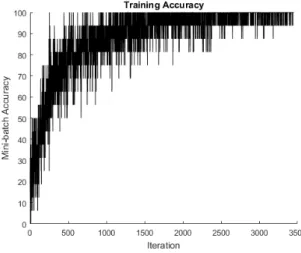
Choosing a size of a mini batch is closely related to the number of epochs (iterations) the network was trained. We trained the neural network for 20 epochs. The size of a mini batch varied from 8, 16, 32, 64 to 128 images. For fixed size of training epochs, the number of iterations was biggest for MBS (mini batch size) 8 –more than 4000, and it was smallest for MBS 128 – below 500. With smaller mini batch the training images are visited many times, so CNN experienced enormous overfitting. From the same reason, overfitting is less for larger mini batches. During training of the network, we introduced an accuracy threshold of 99.5, in order to stop the training process because of the overfitting. The training was stopped in cases when the size of a mini batch was 8 and 16, Figure 6.
The classification accuracy which was achieved with MBS of 128 images and 20 training epochs was 81%. It can reach over 83% when the neural network is trained with MBS of 128 images and 30 training epochs.
Figure 6. Training accuracy with mini batch size of 16 images
0.7767 0.7967 0.8067 0.8117 0.75 0.76 0.77 0.78 0.790.8 0.81 0.82 0.001 0.0005 0.0001 0.00001 A ccur acy L2 regularization parameter
We simulated transfer learning from pre-trained CNN with layer-specific optimization parameter: the learning rate for weights and biases of the neurons of the last fully connected layer. Because ImageNet data and CIFAR-10 are similar data sets, it is reasonable to keep the weights and biases of the layers which we took from AlexNet in a great measure and to make the new fully connected layer to learn more. Fig.7 presents the increasing of the classification accuracy with the growth of the weight and bias learn rate factor.
Figure 7. Accuracy of pre-trained CNN as a function of weight and bias learn factor
5. Concluding remarks
In our research assignment, we tried to solve the problem of classification of a small dataset of images with the technique known as transfer learning. We transferred knowledge from AlexNet and at the same time, we were optimizing the hyper parameters of our network with the purpose to maximize the accuracy on the test data. We got an accuracy of over 85% in specific cases of a simulation scenario.
Neural network training was short in time and the training dataset consisted a couple thousands of images. We didn’t modify the weights too soon and too much. Taking in to consideration the similarity of ImageNet data set and CIFAR-10 dataset, we imported the architecture of AlexNet in a great measure, as far as the weights of all layers (except the last three one) of the pre-trained network.
There are situations when the training and testing set of images are small, and yet we need to classify it with acceptable accuracy. Then comes to a situation when one should think of transfer learning from a pre-trained neural network as an option. In order to get as high as possible classification accuracy, the pre-trained model selected for transfer learning has to be trained on a similar data set as the data set we wish to use it on. If the image set we have to classify differs a lot from the one on which the pre-existing neural network was trained, then the classification would be very inaccurate. There are various architectures people have tried on different types of data sets.
5. References
[1] A. Krizhevsky, I. Sutskever, G. E. Hinton, “ImageNet Classification with Deep Convolutional Neural Networks”, pp. 1106– 1114, 2012
[2] Michael A. Nielsen, “Neural Networks and Deep learning”, Determination Press 2015
[3] Deng, W. Dong, R. Socher, L.-J. Li, K. Li, and L. Fei-Fei, “ImageNet: A Large-Scale Hierarchical Image Database”, In CVPR09, 2009
[4] Wang C, Mahad-evan S, “Heterogeneous Domain Adaptation Using Manifold Alignment”, Proceedings of the 22nd international joint conference on artificial intelligence, vol. 2. 2011. p. 541–46.
[5] Duan L, Xu D, Tsang IW, “Learning with Augmented Features for Heterogeneous Domain Adaptation”, IEEE Trans Pattern Anal Mach Intell 2012; 36(6):1134–48.
[6] Zhu Y, Chen Y, Lu Z, Pan S, Xue G, Yu Y, Yang Q, “Heterogeneous Transfer Learning for Image Classification”, Proceedings of the national conference on artificial intelligence, vol. 2. 2011. p. 1304–9
[7] Harel M, Mannor, “Learning from Multiple Outlooks”, Proceedings of the 28th international conference on machine learning 2011, p. 401–8
[8] Nam J, Kim S, “Heterogeneous Defect Prediction”, Proceedings of the 2015 10th joint meeting on foundations of software engineering, 2015. p. 508–19 0,6383 0,725 0,7933 0,815 0 0,2 0,4 0,6 0,8 1 2;5 5;10 8;15 10;20 A ccu racy
Weight learn rate factor Bias learn rate factor
23 Figure 4. Process of training with different learning rates
Figure 5. Accuracy of pre-trained CNN as a function of L2 regularization parameter
Choosing a size of a mini batch is closely related to the number of epochs (iterations) the network was trained. We trained the neural network for 20 epochs. The size of a mini batch varied from 8, 16, 32, 64 to 128 images. For fixed size of training epochs, the number of iterations was biggest for MBS (mini batch size) 8 –more than 4000, and it was smallest for MBS 128 – below 500.With smaller mini batch the training images are visited many times, so CNN experienced enormous overfitting. From the same reason, overfitting is less for larger mini batches. During training of the network, we introduced an accuracy threshold of 99.5, in order to stop the training process because of the overfitting. The training was stopped in cases when the size of a mini batch was 8 and 16, Figure 6.
The classification accuracy which was achieved with MBS of 128 images and 20 training epochs was 81%. It can reach over 83% when the neural network is trained with MBS of 128 images and 30 training epochs.
Figure 6. Training accuracy with mini batch size of 16 images
0.7767 0.7967 0.8067 0.8117 0.75 0.76 0.77 0.78 0.790.8 0.81 0.82 0.001 0.0005 0.0001 0.00001 A ccur acy L2 regularization parameter
We simulated transfer learning from pre-trained CNN with layer-specific optimization parameter: the learning rate for weights and biases of the neurons of the last fully connected layer. Because ImageNet data and CIFAR-10 are similar data sets, it is reasonable to keep the weights and biases of the layers which we took from AlexNet in a great measure and to make the new fully connected layer to learn more. Fig.7 presents the increasing of the classification accuracy with the growth of the weight and bias learn rate factor.
Figure 7. Accuracy of pre-trained CNN as a function of weight and bias learn factor
5. Concluding remarks
In our research assignment, we tried to solve the problem of classification of a small dataset of images with the technique known as transfer learning. We transferred knowledge from AlexNet and at the same time, we were optimizing the hyper parameters of our network with the purpose to maximize the accuracy on the test data. We got an accuracy of over 85% in specific cases of a simulation scenario.
Neural network training was short in time and the training dataset consisted a couple thousands of images. We didn’t modify the weights too soon and too much. Taking in to consideration the similarity of ImageNet data set and CIFAR-10 dataset, we imported the architecture of AlexNet in a great measure, as far as the weights of all layers (except the last three one) of the pre-trained network.
There are situations when the training and testing set of images are small, and yet we need to classify it with acceptable accuracy. Then comes to a situation when one should think of transfer learning from a pre-trained neural network as an option. In order to get as high as possible classification accuracy, the pre-trained model selected for transfer learning has to be trained on a similar data set as the data set we wish to use it on. If the image set we have to classify differs a lot from the one on which the pre-existing neural network was trained, then the classification would be very inaccurate. There are various architectures people have tried on different types of data sets.
5. References
[1] A. Krizhevsky, I. Sutskever, G. E. Hinton, “ImageNet Classification with Deep Convolutional Neural Networks”, pp. 1106– 1114, 2012
[2] Michael A. Nielsen, “Neural Networks and Deep learning”, Determination Press 2015
[3] Deng, W. Dong, R. Socher, L.-J. Li, K. Li, and L. Fei-Fei, “ImageNet: A Large-Scale Hierarchical Image Database”, In CVPR09, 2009
[4] Wang C, Mahad-evan S, “Heterogeneous Domain Adaptation Using Manifold Alignment”, Proceedings of the 22nd international joint conference on artificial intelligence, vol. 2. 2011. p. 541–46.
[5] Duan L, Xu D, Tsang IW, “Learning with Augmented Features for Heterogeneous Domain Adaptation”, IEEE Trans Pattern Anal Mach Intell 2012; 36(6):1134–48.
[6] Zhu Y, Chen Y, Lu Z, Pan S, Xue G, Yu Y, Yang Q, “Heterogeneous Transfer Learning for Image Classification”, Proceedings of the national conference on artificial intelligence, vol. 2. 2011. p. 1304–9
[7] Harel M, Mannor, “Learning from Multiple Outlooks”, Proceedings of the 28th international conference on machine learning 2011, p. 401–8
[8] Nam J, Kim S, “Heterogeneous Defect Prediction”, Proceedings of the 2015 10th joint meeting on foundations of software engineering, 2015. p. 508–19 0,6383 0,725 0,7933 0,815 0 0,2 0,4 0,6 0,8 1 2;5 5;10 8;15 10;20 A ccu racy
Weight learn rate factor Bias learn rate factor
CLASSIFICATION OF SMALL DATA SETS OF IMAGES WITH TRANSFER LEARNING IN CONVOLUTIONAL NEURAL NETWORKS
24
[9] Zhou JT, Pan S, Tsang IW, Yan Y, “Hybrid Heterogeneous Transfer Learning Through Deep Learning”, Proceedings of the national conference on artificial intelligence, vol. 3. 2014. p. 2213–20.
[10] Pan SJ, Yang Q, “A Survey on Transfer Learning” IEEE Trans Knowl Data Eng 2010; 22(10):1345–59.
[11]Bergstra, J. and Bengio, Y. (2012), “Random Search for Hyper-Parameter Optimization”, J. Machine Learning Res., 13, 281–305.
[12]Courville, A., Bergstra, J., and Bengio, Y. (2011), “Unsupervised Models of Images by Spike-And-Slab RBMs”, In ICML’2011
[13]Alex Krizhevsky, “Learning Multiple Layers of Features from Tiny Images”, 2009
[14]www.analyticsvidhya.com, https://www.analyticsvidhya.com/blog/2017/06/transfer-learning-the-art-of-fine-tuning-a-pre-trained-model/
[15]www.innoarchitech.com, https://www.innoarchitech.com/artificial-intelligence-deep-learning-neural-networks-explained/ [16]Bengio, Y. (2012), “Practical Recommendations for Gradient-Based Training of Deep Architectures”, arXiv: 1206.5533V2
[cs.LG] 16 Sep 2012
[17]Zeiler, M. D., and Fergus, R. “Visualizing and understanding convolutional networks”, CoRR, abs/1311.2901, 2013. Published in Proc. ECCV, 2014
[18]Sermanet, P., Eigen, D., Zhang, X., Mathieu, M., Fergus, R., and LeCun, Y. OverFeat: “Integrated Recognition, Localization and Detection using Convolutional Networks”. In Proc. ICLR, 2014.
[19]Simonyan, K. and Zisserman, A. “Two-stream convolutional networks for action recognition in videos”. CoRR, abs/1406.2199, 2014. Published in Proc. NIPS, 2014
[20]Dean, J., Corrado, G., Monga, R., Chen, K., Devin, M., Mao, M., Ranzato, M., Senior, A., Tucker, P., Yang, K., Le, Q. V., and Ng, A. Y. “Large scale distributed deep networks”. In NIPS, pp. 1232–1240, 2012
[21]Russakovsky, O., Deng, J., Su, H., Krause, J., Satheesh, S., Ma, S., Huang, Z., Karpathy, A., Khosla, A., Bernstein, M., Berg, A. C., and Fei-Fei, L. “ImageNet large scale visual recognition challenge”. CoRR, abs/1409.0575, 2014.
[22]Perronnin, F., Sa´nchez, J., and Mensink, T. “Improving the Fisher kernel for large-scale image classification”. In Proc. ECCV, 2010.
WEB SERVICE BASED GENOMIC DATA RETRIEVAL
Done Stojanov
Faculty of computer science, Goce Delcev University, Stip, Macedonia [email protected]
Abstract: An application of web service for genomic data retrieval is considered. Records for nucleotide sequences are retrieved from the European Nucleotide Archive and preprocessed locally in order to be able to apply local host based analysis. This analysis is required because many of the built-in EMBL-EBI services pose restrictions upon the metrics with which will operate the user, what in some cases may also affect the structure of the solution, such as when performing pairwise or multiple DNA or mRNA comparison. Keywords: web, service, data, retrieval, ENA
1.
Introduction
In recent years, a huge volume of genomic data has been accessed. This was possible due to the advances in the DNA sequencing techniques, such as shotgun sequencing and bridge PCR technique. The value of the collected DNA information increases by sharing in the scientific community. This idea drove the construction of the central repository of nucleotide data: ENA or The European Nucleotide Archive [1].
ENA or The European Nucleotide Archive (web access: https://www.ebi.ac.uk/ena) [1] is a public database hosted under the European Bioinformatics Institute (EMBL-EBI) [2] that contains records for nucleotide sequences. ENA allows upload/access/download of nucleotide data derived from different sources (organisms) applying different sequencing techniques.
ENA evolved from the EMBL Data Library which was officially released in 1982 [3] and it contained 568 records with total size of 500,000 base pairs [4]. Since then the volume of the data in this repository exponentially grows [5].
Data stored in this repository is functionally annotated. This means that in spite of the exact order of nucleotides in the sequence, data linkage details are also available. For instance, when accessing a whole genome, each CDS (coding sequence) is differentiated from other coding frames, as well as from non-coding frames. By knowing the start and the end of each CDS, the structure of the mRNA being transcribed and the protein being translated can be exactly determined.
Regardless record’s functional association, there is metadata common for all. This means that regardless the record is associated to a whole genome, chromosome or partial CDS (partial coding region or partial mRNA) there are descriptors which are common for all records.
For each record there is information that describes: the source (organism) of nucleotide sequence, type and topology of the molecule, taxonomic division or taxonomic rank (ex. HUM (Human), PRO (Prokaryote)…etc.), length of the sequence or the number of base pairs, sequence version, date when the sequence was made public and the date of last update of the sequence. Keywords that describe the sequence and secondary accession information are also available.
However, the most important feature of each record in ENA is that there is no restriction in the accession of exact structure of nucleotide sequence. This information can be accessed in three data formats: TEXT, FASTA and
XML.
The European Bioinformatics Institute (EMBL-EBI) also hosts web implementations of the most popular algorithms for genomic data analysis, such as: EMBOSS Needle – an implementation of the Needleman-Wunsch algorithm [6], EMBOSS Water – an implementation of the Smith-Waterman algorithm [7], EMBOSS Matcher – an
![Figure 1. Transfer learning according to the characteristics of dataset [14]](https://thumb-us.123doks.com/thumbv2/123dok_us/10012155.2493600/9.892.321.567.744.991/figure-transfer-learning-according-characteristics-dataset.webp)
![Figure 1. Transfer learning according to the characteristics of dataset [14]](https://thumb-us.123doks.com/thumbv2/123dok_us/10012155.2493600/10.892.122.839.726.943/figure-transfer-learning-according-characteristics-dataset.webp)