Generation and detection of nonlinear Lamb waves for the characterization of material nonlinearities. Christian Bermes

(1)

Generation and detection of nonlinear Lamb waves

for the characterization of material nonlinearities

A Thesis Presented to The Academic Faculty

by

Christian Bermes

In Partial Fulfillment

of the Requirements for the Degree

Master of Science in Engineering Science and Mechanics

School of Civil and Environmental Engineering Georgia Institute of Technology

(2)

Generation and detection of nonlinear Lamb waves

for the characterization of material nonlinearities

Approved by:

Dr. Laurence J. Jacobs, Advisor School of Civil and Environmental Engineering

Georgia Institute of Technology Dr. Jianmin Qu

George W. Woodruff School of Mechanical Engineering

Georgia Institute of Technology Dr. Jin–Yeon Kim

George W. Woodruff School of Mechanical Engineering

Georgia Institute of Technology Date Approved: August 23, 2006

(3)

(4)

ACKNOWLEDGEMENTS

My sincere gratitude is expressed towards everyone who has supported me in the making of this thesis and in my studies over the past five years.

I would especially like to thank my academic advisor Prof. Laurence J. Jacobs for all his support, inspiration and advice. Due to his great organizational and financial efforts I received the opportunity to present the results of this thesis at the QNDE conference in Portland, Oregon. During my stay at Georgia Tech he has become my mentor and good friend, and I will truly miss our conversations during many morning runs.

Dr. Jin–Yeon Kim is the mastermind behind all my experiments, guiding me in the right direction and showing me the way out whenever I thought I was stuck. I cannot thank him enough for his advice.

Moreover I would like to thank Prof. Jianmin Qu for his unpayable advice and for granting access to the facilities of the School of Mechanical Engineering and Krit-sakorn Luangvilai for his patient introduction to the laser interferometer. Thanks go also to my predecessor Jan Herrmann, who answered all my questions regarding the measurement system. With his assistance in the lab, Prof. Guoshuang Shui alleviated my experimental work enormously.

For their friendship, their moral support and the fruitful discussions at work I ex-press my gratitude to my lab fellows Florian J. Kerber, J¨urgen Koreck, Kritsakorn Luangvilai, H. Benjamin Mason and Dr. Wonsiri Punurai. Moreover, I would like to thank Dr. Christine Valle for bringing fresh spirit into the lab and sacrificing her time to review my written work.

(5)

Exchange Program between the University of Stuttgart and the Georgia Institute of Technology as well as Dr.–Ing. Matthias Maess, who put a lot of time and effort in his exemplary support and advice for his exchange students. The generous fundings of the German Academic Exchange Service (DAAD) and the German National Aca-demic Foundation are gratefully acknowledged.

Finally, I am deeply indebted to my parents, who support me in an unprecedented way and always have faith in my intentions and plans. Their loving encouragement always accompanies me.

(6)

LIST OF TABLES

Table 2.1 Angle relations for reflection on a stress–free surface. . . 10 Table 3.1 Material properties of aluminum 6061–T6 and aluminum 1100–H14. 29 Table 3.2 Two cumulative second harmonic excitation setpoints of aluminum

6061–T6 and aluminum 1100–H14 for a plate thickness of 1 mm. . 31 Table 6.1 Best fit curve parameters and relative nonlinearity parameter ratios. 68 Table B.1 Amplitudes for the measurements in aluminum 6061–T6 evaluated

with STFT. . . 82 Table B.2 Amplitudes for the measurements in aluminum 6061–T6 evaluated

with chirplet. . . 83 Table B.3 Amplitudes for the measurements in aluminum 1100–H14

evalu-ated with STFT. . . 83 Table B.4 Amplitudes for the measurements in aluminum 1100–H14

(9)

LIST OF FIGURES

Figure 1.1 Cumulative second harmonic generation and tracking of

nonlinear-ity parameter with fatigue life for Rayleigh waves [13]. . . 2

Figure 2.1 Momentum balance. . . 5

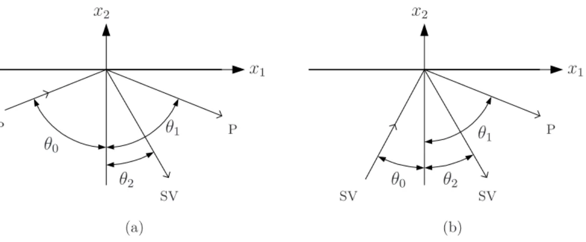
Figure 2.2 Wave reflections. (a) Reflection of a P–wave. (b) Reflection of an SV–wave. . . 10

Figure 2.3 Multiple reflections in a waveguide. . . 11

Figure 2.4 Theoretical solution in the phase velocity – frequency domain (dis-persion curves). . . 13

Figure 2.5 Theoretical solution for the Lamb wave. . . 14

Figure 2.6 Linear and nonlinear wave propagation in a solid. . . 15

Figure 3.1 Cumulative second harmonic excitation setpoint s1 →s2. . . 30

Figure 3.2 Cumulative second harmonic excitation setpoint s2 →s4. . . 30

Figure 4.1 Generation of a Lamb wave with the wedge method. . . 33

Figure 4.2 Improved wedge design including a clamping tip (not to scale). . 35

Figure 4.3 Laser interferometer detection system. . . 37

Figure 4.4 Experimental setup. . . 42

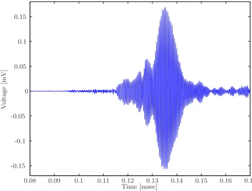
Figure 5.1 Typical time signal with overlapping Lamb modes. . . 45

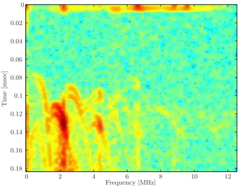
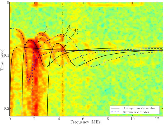
Figure 5.2 Typical spectrogram for the performed measurements. . . 46

Figure 5.3 Spectrogram and dispersion curves. . . 47

Figure 5.4 Fundamental and second harmonic frequency as functions of time. 48 Figure 5.5 CT basis functions adjusted to the s0–mode (fifth–order approxi-mation) [18]. . . 49

Figure 5.6 Amplitude plot of the CT for the s0–mode in an aluminum plate [18]. 50 Figure 6.1 Relative nonlinearity parameterβ′ _{as functions of transducer input} voltage evaluated with STFT. . . 52

Figure 6.2 Relative nonlinearity parameter β′⋆ as functions of transducer in-put voltage evaluated with STFT. . . 53

Figure 6.3 Theoretical and measured decay of amplitude A1 as a function of propagation distance. . . 54

(10)

Figure 6.4 Theoretical and measured decay of amplitude A2 as a function of

propagation distance. . . 55 Figure 6.5 Theoretical and measured decay of amplitude A⋆

2 as a function of

propagation distance. . . 56 Figure 6.6 Relative nonlinearity parameter β′ _{as function of propagation}

dis-tance for aluminum 6061–T6 evaluated with STFT (see Table B.1 for corresponding data). . . 58 Figure 6.7 Relative nonlinearity parameterβ′⋆

as function of propagation dis-tance for aluminum 6061–T6 evaluated with STFT (see Table B.1 for corresponding data). . . 59 Figure 6.8 Relative nonlinearity parameter β′ _{as function of propagation}

dis-tance for aluminum 6061–T6 evaluated with chirplet (see Table B.2 for corresponding data). . . 60 Figure 6.9 Relative nonlinearity parameterβ′⋆

as function of propagation dis-tance for aluminum 6061–T6 evaluated with chirplet (see Table B.2 for corresponding data). . . 61 Figure 6.10 Relative nonlinearity parameter β′ _{as function of propagation}

dis-tance for aluminum 1100–H14 evaluated with STFT (see Table B.3 for corresponding data). . . 62 Figure 6.11 Relative nonlinearity parameterβ′⋆

as function of propagation dis-tance for aluminum 1100–H14 evaluated with STFT (see Table B.3 for corresponding data). . . 63 Figure 6.12 Relative nonlinearity parameter β′ _{as function of propagation}

dis-tance for aluminum 1100–H14 evaluated with chirplet (see Ta-ble B.4 for corresponding data). . . 64 Figure 6.13 Relative nonlinearity parameterβ′⋆

as function of propagation dis-tance for aluminum 1100–H14 evaluated with chirplet (see Ta-ble B.4 for corresponding data). . . 65 Figure 6.14 Comparison of relative nonlinearity parametersβ′ _and _β′⋆

as func-tions of propagation distance for both alloys evaluated with STFT. 66 Figure 6.15 Comparison of relative nonlinearity parametersβ′ _and _β′⋆

as func-tions of propagation distance for both alloys evaluated with chirplet. 67 Figure A.1 Visualization of operators for the chirplet transform [18]. . . 80

(11)

SUMMARY

An understanding of the generation of higher harmonics in Lamb waves is of critical importance for applications such as remaining life prediction of plate–like structural components. The objective of this work is to use nonlinear Lamb waves to experimentally investigate inherent material nonlinearities in aluminum plates. These nonlinearities, e.g. lattice anharmonicities, precipitates or vacancies, cause higher har-monics to form in propagating Lamb waves. The amplitudes of the higher harhar-monics increase with increasing propagation distance due to the accumulation of nonlinear-ity while the Lamb wave travels along its path. Special focus is laid on the second harmonic, and a relative nonlinearity parameter β′ _{is defined as a function of the} fundamental and second harmonic amplitude. The experimental setup uses an ultra-sonic transducer and a wedge for the Lamb wave generation and laser interferometry for detection. The experimentally measured Lamb wave signals are processed with a short–time Fourier transformation (STFT) and a chirplet transformation–based al-gorithm, which yield the amplitudes of the frequency spectrum as functions of time, allowing the observation of the nonlinear behavior of the material. The increase ofβ′ with propagation distance as an indicator of cumulative second harmonic generation is shown in the results for two different aluminum alloys. The difference in inherent nonlinearity between both alloys as determined from longitudinal wave measurements can be observed for the Lamb wave measurements, too.

(12)

CHAPTER I

INTRODUCTION

Nonlinear ultrasound has proven to be a very useful technique in nondestructive eval-uation (NDE) to track the damage condition in structural components even before the initiation of the first crack. In comparison to classical NDE techniques, where damage evaluations are based on the crack–scattered wavefield, nonlinear ultrasound has the potential to enable assessments of the current damage state much earlier. For damage types based on plastic deformation, such as fatigue and creep damage, nonlinear ultrasonic methods offer an especially high potential for qualitative and quantitative investigations.

The physical effect that is monitored in nonlinear ultrasonic measurements is the generation of higher harmonic frequencies in an originally single frequency wave pro-pagating in the sample. This higher harmonic generation appears due to the nonlin-earity of the component’s material, which is described with a nonlinear stress–strain relationship. The material nonlinearity consists of two sources: the inherent, nat-ural material nonlinearity and damage induced nonlinearity. In addition to these, the possibility of nonlinearity introduced by the experimental setup always has to be investigated.

In order to quantify the degree of nonlinearity present in a material, a nonlinearity parameter β can be used. Theoretically, β is described in terms of the higher order elastic constants from the nonlinear stress–strain relationship and represents a dis-tinct material property. However, the absolute value of β can only be determined experimentally. Cantrell and Yost, for instance, have determined absolute values of

(13)

of nonlinearity changes from an undamaged to a damaged specimen, the value of β

changes accordingly. Previous publications show thatβ is significantly more sensitive to changes in the material microstructure than linear ultrasonic properties like group velocity, phase velocity or attenuation. Changes in β associated with damage have been shown again by Cantrell and Yost [4] and by Nagy [24] for aluminum.

In the work of Herrmann et al. [13], Rayleigh surface waves are used to show cumula-tive second harmonic generation with propagation distance in Nickel–based superal-loys. Moreover, the specimens are damaged in low cycle fatigue tests and nonlinearity parameter and specimen fatigue life are tracked simultaneously. The transition from verifying the inherent material nonlinearity to damaging the specimen and success-fully tracking nonlinearity as a function of damage state is shown in Figure 1.1. Based

3.0 3.2 3.4 3.6 3.8 4.0 4.2 4.4 4.6 4.8 0.0000 0.0005 0.0010 0.0015 0.0020 0.0025 0.0030 0.0035 N o rm a liz e d a m p lit u de o f h ig h e r h a rm o n ic s , A 'n /A '1 Propagation distance (cm)

Second order harmonic Third order harmonic Linear fit 0 10 20 30 40 50 60 70 80 90 100 1.0 1.1 1.2 1.3 1.4 1.5

1.6 Longitudinal wave measurement (Specimen #1) Longitudinal wave measurement (Specimen #2) Rayleigh wave measurement (Specimen #1) Rayleigh wave measurement (Specimen #2) Best fit of longitudinal wave measurement results

N o rm a liz e d a c o u s ti c n o n lin e a ri ty , E / Eun fa t Fatigue life (%)

Figure 1.1: Cumulative second harmonic generation and tracking of nonlinearity parameter with fatigue life for Rayleigh waves [13].

on the displayed results, lifetime prediction by tracking the nonlinearity parameter of a specimen is possible, even before the initiation of the first macroscopic crack. The wave types successfully used so far are longitudinal waves [19] and Rayleigh surface waves [13].

The fundamental idea of this work is to perform similar nonlinear ultrasonic mea-surements with Lamb waves. As guided wave, this wavetype appears promising for

(14)

the interrogation of plate–like structures in possible field applications. However, ap-plication of Lamb waves to nonlinear ultrasonic measurements is significantly more difficult compared to the wave types previously mentioned. The reasons for this higher degree of difficulty lie in two facts: Lamb waves are dispersive, which means that phase and group velocity are functions of frequency, and Lamb waves are a multi–modal wavetype, having several modes propagating simultaneously. Because of that, cumulative higher harmonic generation in Lamb waves is only possible under certain, very restrictive conditions. The work of Deng derives and explains these conditions in detail [6, 7, 8] and also shows some experimental validation of the the-oretical work [9]. Due to these complications, the goal of this research is limited to verifying the inherent material nonlinearity of two different aluminum alloys, alu-minum 6061–T6 and alualu-minum 1100–H14, whose absolute nonlinearity parameters are known from longitudinal wave measurements [31]. The combination of contact wedge generation and non–contact laser interferometric detection is used as an exper-imental setup for the Lamb wave measurements. With this, the dependence of higher harmonic generation on wave propagation distance in the specimen is investigated. It is attempted to comply experimentally with the analytical relationship between the amount of nonlinearity and the propagation distance. A simultaneous tracking of damage and nonlinearity is postponed to future work.

In Chapter 2, an overview of the fundamental theory of linear wave propagation in elastic solids is given. Furthermore, in the theory of nonlinear wave propagation, the nonlinearity parameter β is derived for longitudinal waves and subsequently corre-lated to higher harmonic generation in Lamb waves. Chapter 3 presents the detailed derivation of the conditions for the excitation of cumulative second harmonics in Lamb waves according to [6]. Subsequently, in Chapter 4 the experimental setup for the Lamb wave measurements is shown. Contact wedge generation and non–contact laser interferometric detection are explained as well as the overall setup including the

(15)

specimens used. Since careful signal processing has to be applied in order to identify the desired harmonic amplitudes from the measured signals, Chapter 5 is dedicated to the two methods that are applied for signal processing, namely short–time Fourier transformation and adaptive chirplet algorithm. Their fundamental theory can be found in Appendix A. In Chapter 6, the results from the measurements after signal processing are presented. The results comprise checks for plate spreading and in-strumentation nonlinearity, and the developing of the nonlinearity parameter of both aluminum alloys as a function of propagation distance is shown. Moreover, a com-parison is made between the two alloys aluminum 6061–T6 and aluminum 1100–H14. Finally, the results are summarized and discussed in Chapter 7. An outlook on open questions and future work is given as well.

(16)

CHAPTER II

FUNDAMENTAL THEORY

To conduct this research, a thorough understanding of the theoretical fundamentals is indispensable. Thus, an introduction to linear and nonlinear wave propagation is given in this chapter.

2.1 Linear wave propagation

The theory of linear wave propagation is well–known and –documented, good sources are for instance Achenbach [1] and Graff [11]. The following sections will briefly describe the fundamental aspects of linear wave propagation. Additionally, wave phenomena like reflections are discussed. Finally, the key wave type for this research, i.e. Lamb waves, will be explained.

2.1.1 Equations of motion

To derive the equations of motion, consider a volume V at time t bounded by the surface S (see Figure 2.1). As a result of the momentum principle, the time rate of

dV S V ρbdV tdS dS

Figure 2.1: Momentum balance.

(17)

the external forces.

For the total momentum of the given mass, the momentum change is given as

d dt

R

ρvidV, with _dtd being the material derivative of the integral. The momentum

balance is then described as

Z S tidS+ Z V ρbidV = d dt Z V ρvidV, (2.1)

where ti are the surface tractions, bi are the body forces and v is the velocity. Next,

substitution of the Cauchy formula

ti =σijnj (2.2)

in the momentum balance (2.1) and transformation of the surface integral using the divergence theorem leads to

Z

V

[σij,j+ρbi−ρv˙i]dV = 0. (2.3)

In order to transfer the material derivative inside the integral, the Reynolds formula is employed. Equation (2.3) holds for any arbitrary volume, hence it is possible to state

σij,j+ρbi =ρv˙i . (2.4)

These are Cauchy’s equations of motion. Note, that the stress tensorσij is symmetric.

The equations of motion can also be expressed solely in terms of the displacements

ui. Hooke’s law for a homogeneous, isotropic and linear elastic medium needs to be

assumed for the volume V:

σij =λǫkkδij + 2µǫij, (2.5)

with ǫij being the strain tensor related to the displacements ui by

ǫij =

1

(18)

From that, Navier’s equation of motion can be obtained as

µui,jj+ (λ+µ)uj,ji = ρu¨i (2.7)

µ_∇2u+ (λ+µ)_{∇∇ ·}u = ρu¨, (2.8)

where λ and µ are the Lam´e constants. In this derivation, the body forces are neglected.

The coupled partial differential equation (2.8) can be uncoupled with the Helmholtz decomposition

u=_∇ϕ+_{∇ ×}ψ. (2.9)

Equation (2.9) represents the three components of the displacement u in terms of the four potential functions ϕ, ψ1, ψ2 and ψ3. An additional constraint is required in

order to guarantee the uniqueness of the solution:

∇ ·ψ= 0. (2.10)

By substituting the Helmholtz decomposition (2.9) into the displacement equations of motion (2.8), two uncoupled wave equations expressed in terms of the displacement potentials ϕ and ψ are obtained:

∇2ϕ = 1 c2 L ¨ ϕ, (2.11) ∇2ψ = 1 c2 T ¨ ψ. (2.12)

The wave speed of the longitudinal wave (also called dilatational, irrotational, pressure or P–wave) is denoted by cL, while the wave speed of the vertically and horizontally

polarized shear waves (also called transverse, rotational, distortional or S–waves) is represented by cT. In terms of the material properties, the wave speeds are defined

as

c2_L = λ+ 2µ

(19)

and

c2_T = µ

ρ . (2.14)

Equations (2.11)–(2.12) represent the general form of the wave equation and will still hold if the potentials are replaced by the displacements or the strains.

From comparison of the numerators in equations (2.13)–(2.14) it follows immediately that cL > cT. Finally, the Lam´e constants λ and µ are related to the material’s

Young’s modulus E and Poisson’s ratio ν by

λ = Eν

(1 +ν)(1₋2ν) , (2.15)

µ = E

2(1 +ν) . (2.16)

2.1.2 Wave phenomena

The basis of all wave phenomena discussed in this section is the plane wave assump-tion. That means that a wave with constant properties (ǫ, σ, u) is assumed on a plane perpendicular to its direction of propagation p (propagating vector). A plane wave is represented mathematically as

u=df(x_·p₋ct), (2.17)

withdbeing the unit vector that defines the direction of particle motion (displacement vector), andcbeing either the longitudinal wave speedcLor the transverse wave speed cT. Substitution of (2.17) into Navier’s equation of motion (2.8) yields

(µ₋ρc2)d+ (λ+µ)(p_·d)p= 0. (2.18)

Because p and d are two different unit vectors, two solutions to (2.18) are possible. These solutions are eitherd=_±porp_·d= 0 and form the basis of wave propagation. Two cases can be distinguished according to the two solutions:

(20)

(1) The solution d = _±p immediately leads to p_·d = _±1. Evaluation of (2.18) yieldsc=cL as defined in (2.13). Sincedandpare linearly dependent, this

rep-resents a particle movement in the direction of propagation, which corresponds physically to a longitudinal or P–wave.

(2) The solutionp _·d= 0 leads with (2.14) and (2.18) to c=cT. Hence, the

direc-tion of modirec-tion is normal to the direcdirec-tion of propagadirec-tion, and the wave is called a transverse or S–wave. If a two–dimensional plane of propagation is consid-ered (for example, the (x1, x2)-plane), a wave with an in–plane displacement (in

the (x1, x2)-plane) is called SV–wave (vertically polarized), while a wave with

out–of–plane displacement (in thex3–direction) is called SH–wave (horizontally

polarized).

In a homogeneous, isotropic material, transverse and longitudinal wave speeds are independent of frequency, therefore they are nondispersive.

In an infinite medium, the wave types derived so far propagate independently. How-ever, as soon as a finite medium in the direction of propagation is considered, re-flections and coupling will occur due to the presence of boundaries. If an incident P–wave is reflected at a stress free boundary (σ22 = 0 and σ21 = 0), it will normally

cause both a reflected P–and SV–wave. Similarly, if an incident SV–wave is reflected at a stress free boundary, it will generally cause both reflected SV–and P–waves. This effect is known as mode conversion. In Figure 2.2, the reflections of an incident P–and SV–wave are illustrated.

The displacement field of a harmonic wave in the (x1, x2)–plane (propagating in

infinite media, plane–strain case) can be expressed as

u(n)=And(n)exp

h

ıkn(x1p(n)1 +x2p(n)2 −cnt)

i

, (2.19)

where n denotes the wave characteristics (longitudinal or transverse) and kn = _cω_n is

(21)

P P SV x1 x2 θ0 θ1 θ2 (a) P SV SV x1 x2 θ0 θ1 θ2 (b)

Figure 2.2: Wave reflections. (a) Reflection of a P–wave. (b) Reflection of an SV– wave.

definitions, the fact that the angular frequency ω is equal for the incident and the reflected waves, and the interface boundary conditions make it possible to determine the relationship between the angle of the incident and the angles of the reflected waves. These relationships are summarized in Table 2.1. In order to obtain non–

Table 2.1: Angle relations for reflection on a stress–free surface. incidentθ0 reflected P θ1 reflected SV θ2

P θ1 =θ0 sinθ2 = (cT/cL) sinθ0

SV sinθ1 = (cL/cT) sinθ0 θ2 =θ0

trivial amplitudes An, the angles of incident and reflected waves θ0, θ1 and θ2 (see

Figure 2.2) have to satisfy Snell’s law:

k0sinθ0 =k1sinθ1 =k2sinθ2 . (2.20)

Two exceptions exist for mode conversion: firstly, at normal incidence with θ0 = 0

the incident waves are reflected as themselves. Secondly, if the angle θ0 is greater

than a critical angle

θcritical = arcsin cT cL

(22)

only an SV–wave is reflected. In this case, the P–wave portion of the reflected signal degenerates into a Rayleigh surface wave, a specific type of two–dimensional harmonic wave.

2.1.3 Lamb waves

Lamb waves belong to the class of guided waves, which travel in a body (the wave-guide) with at least one, but usually two boundaries. As illustrated in Figure 2.1.3, waves are reflected at two surfaces, causing them to propagate back and forth between the surfaces and producing multiple reflections at each of them. Due to the mode conversion at these boundaries, multiple propagating waves are generated, causing an interference pattern in the waveguide. The result of this effect is that propagating waves are guided in a certain direction.

x₁

x2

2h P SV SV P

Figure 2.3: Multiple reflections in a waveguide.

In order to model the phenomenon of guided waves, the following complex potentials are assumed:

ϕ= Φ(x2)eı(kx1−ωt), ψ = Ψ(x2)eı(kx1−ωt). (2.22)

The additional assumption of the x1–direction as propagation direction and plane

strain stress free boundaries atx2 =±hleads to the Rayleigh–Lamb frequency

equa-tions as they can be found in Achenbach [1]: tan(qh)

tan(ph) =−

4k2_pq

(23)

and tan(qh) tan(ph) =− (q2₋_k2₎2 4k2_pq , (2.24) with p2 = ω 2 c2 L −k2, q2 = ω 2 c2 T −k2. (2.25)

Equation (2.23) represents the symmetric Lamb modes and equation (2.24) represents the antisymmetric Lamb modes, while the thickness of the waveguide accounts for 2h. The terms symmetric and antisymmetric are used with respect to the direction of propagationp, in this case thex1–direction, and describe the amplitude distribution

over the plate thickness. Every Lamb mode propagates with a frequency ω and a phase velocity cph = ω_k. Since the mode velocities change with frequency, the nature

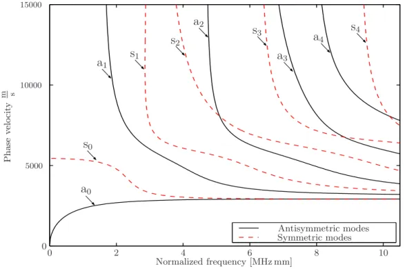
of Lamb waves is called dispersive. Solutions for the Rayleigh–Lamb equations can only be found numerically and are depicted in Figure 2.4. The displayed solutions have been computed with the software Disperse1_{. Further information about the}

program can be found in [27]. The symmetric modes obtained from equation (2.23) are labeled si, i = 0...4, the antisymmetric modes obtained from equation (2.24) are

labeled ai, i= 0...4. To obtain these solutions, first of all a numerical solution in the

(ω, k) domain (and withf = ω

2π in the (f, k) domain, respectively) is determined, and

subsequently f is differentiated partially with respect to the wave number k for all modes. This derivative is again taken numerically and is referred to as group velocity

cg(f):

cg(f) = 2π ∂f

∂k. (2.26)

The group velocity describes the velocity of the energy propagating with the wave and does therefore have a physical meaning. In contrast to that, the phase velocitycph= ω_k

(24)

5000 10000 15000 0 0 2 4 6 8 10 a0 a1 a2 a3 a4 s0 s1 s2 s3 s4 Normalized frequency [MHz mm] P h a se v el o ci ty m s Antisymmetric modes Symmetric modes

Figure 2.4: Theoretical solution in the phase velocity – frequency domain (dispersion curves).

refers to the velocity of points with constant phase. Note, that for nondispersive , i.e. infinitely linearly elastic media, group and phase velocity are equal.

From Equation (2.26), the energy slowness sle(f) is defined as

sle(f) =

1

cg(f)

. (2.27)

In order to obtain a theoretical solution in the time–frequency domain, the relation-ship

t(f) = sle(f)

d (2.28)

represents the expected arrival time for a specific mode at frequency f with a propa-gation distance of d between sender and receiver.

Existing Matlab code is modified to perform a normal mode expansion and calcu-late theoretical Lamb waves for a pcalcu-late that is 1 mm thick and considered infinite. The waveform of the theoretical Lamb waves is obtained by superposition of the

(25)

first six symmetric and anti–symmetric modes with a modeled sampling frequency of 100 MHz. Further information about how to implement dispersion curves, expand the normal modes and obtain formulae for the theoretical Lamb wave is given by Pao [30]. Figure 2.5 depicts the results for the theoretical Lamb wave.

0 0 20 40 60 80 100 -1.5 -1 -0.5 0.5 1 1.5 x 10 -6 Time [µsec] O u t– of –p la n e d is p la ce m en t uz [m ]

Figure 2.5: Theoretical solution for the Lamb wave.

2.2 Nonlinear wave propagation

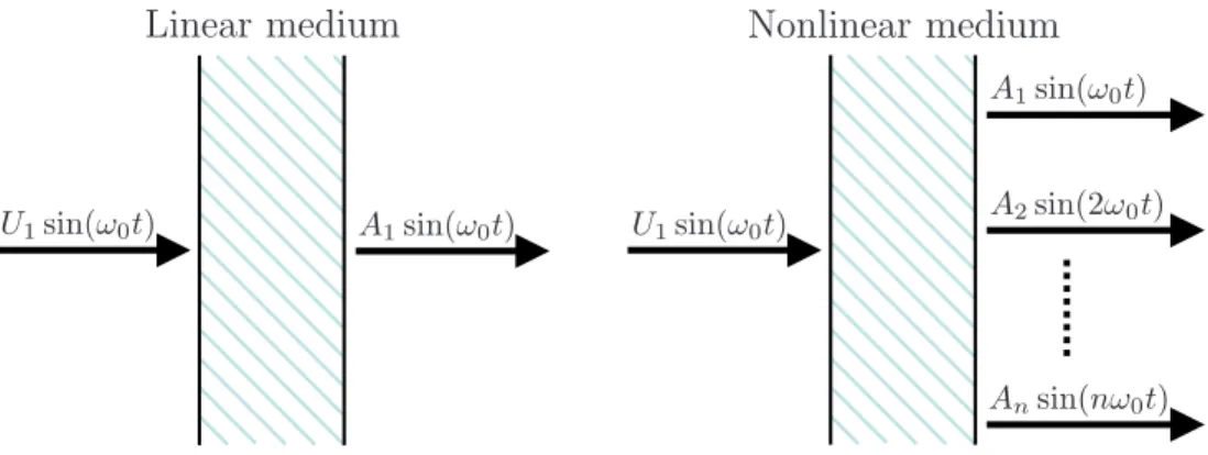
The aim of this section is to give an introduction to one–dimensional nonlinear wave propagation. This is, together with Chapter 3, the theoretical foundation for the ex-perimental part of this thesis. Figure 2.6 schematically shows the difference between linear and nonlinear wave propagation in a solid. While for the linear case the pro-pagating wave travels at only one frequency, the fundamental excitation frequency, in the nonlinear case the material nonlinearities create additional frequencies (the higher harmonics) that are integer multiples of the fundamental frequency. Phys-ically, material nonlinearities are either material inherent (natural), or damage in-duced. Material inherent nonlinearities are e.g. lattice anharmonicities, precipitates or vacancies, whereas damage induced nonlinearities are for instance dislocations or

(26)

Linear medium Nonlinear medium

U1sin(ω0t) A1sin(ω0t) U1sin(ω0t)

A1sin(ω0t)

A2sin(2ω0t)

Ansin(nω0t)

Figure 2.6: Linear and nonlinear wave propagation in a solid.

even microcracks. In terms of the higher harmonics, the observation of the second harmonic, which possesses exactly twice the frequency of the fundamental wave, will be the focal point in the course of this thesis.

An absolute nonlinearity parameter β is introduced in the following. It is a quantity that represents the degree of nonlinearity in a material and is an absolute material related value for undamaged materials. As soon as damage due to plastic deformation occurs, an increase ofβ beyond its material inherent value is observable [12]. For the experimental determination of the absolute parameter β, an expression in terms of the amplitudes of the fundamental and second harmonic frequency is derived. How-ever, it is important to note that this expression holds exclusively for longitudinal wave measurements and only serves as a justification for the introduction of a rela-tive nonlinearity parameter β′ _{for Lamb waves at the end of the section.}

As stated in [14], a wave propagating at a certain fundamental frequency will be distorted in the supporting nonlinear medium. This distortion, particularly caused by lattice anharmonicity and dislocation structures, leads to the generation of higher harmonic frequencies. The generation and growth of the amplitude of the second harmonic frequency contribute to the nonlinearity parameter β, which is derived in

(27)

detail in [3]. In the following, the important steps of this derivation will be summa-rized.

In a solid medium, the longitudinal stress perturbation ¯σ, caused for instance by a propagating ultrasonic wave, leads to a longitudinal strain

ǫ=ǫe+ǫpl, (2.29)

withǫe being the elastic strain component and ǫplbeing the plastic strain component

associated with the motion of dislocations in the dipole configuration. Stress pertur-bation ¯σ and elastic strain component ǫe are related by the nonlinear Hooke’s law

using the quadratic nonlinear approach

¯

σ =Ae₂ǫe+

1 2A

e

3ǫ2e+ higher order terms (h.o.t.) (2.30)

or ǫe= 1 Ae 2 ¯ σ₋1 2 Ae 3 (Ae 2)3 ¯ σ2+ h.o.t. . (2.31) The coefficients Ae

2 and Ae3 are the Huang coefficients [15] and are also referred to as

the initial stress configuration.

The relationship between the stress perturbation ¯σ and the plastic strain component

ǫpl can be found by considering the dipolar forces [3]. The force per unit length along

the glide plane (also referred to as shear force per unit length) for edge dislocation pairs with opposite polarity is given by

¯ Fx1 =− Gb2 2π(1₋ν) x1(x21−x22) (x2 1+x22)2 , (2.32)

whereGis the shear modulus, bis the Burgers vector, νis Poisson’s ratio andx1 and x2 are the Cartesian coordinates of one dislocation pair relative to the other. It is

assumed that motion in dipole pairs occurs only along parallel slip planes separated by the so–called equilibrium dipole height x2 =h. A shear force of bRσ¯ per unit length

(28)

is obtained by resolving the stress perturbation ¯σ along the slip planes, leading to an equilibrium condition of

¯

Fx1 +bRσ¯ = 0. (2.33)

R is the longitudinal–to–shear conversion factor, which is also referred to as Schmid factor.

Furthermore, the relationship between the plastic strain component ǫpl and the

rela-tive dislocation displacement ¯ζ =x₋h can be expressed as

ǫpl= ΩΛdpbξ. (2.34)

In that equation, Ω denotes the conversion factor from the dislocation displacement in the slip plane to a longitudinal displacement along an arbitrary direction, while Λdp _{represents the dipole density. Expanding equation (2.32) in a power series and}

using the relationships (2.33)–(2.34) with ¯ζ =x₋h leads to

¯ σ =Adp₂ ǫpl+ 1 2A dp 3 ǫ2pl+ h.o.t. , (2.35) where Adp2 =− G 4πΩRΛdp_h2₍₁₋_ν₎ , Adp3 = G 4πΩ2_R_(Λdp₎2_h3₍₁₋_ν₎_b . (2.36)

Solving for ǫpl yields the inverse relationship

ǫpl= 1 Adp₂ ¯σ− 1 2 Adp₃ (Adp₂ )3σ¯ 2 _{+ h}_._o_._t_{. .} _(2.37)

Finally, insertion of equations (2.31) and (2.37) into equation (2.29) leads to

ǫ= 1 Ae 2 + 1 Adp₂ ¯ σ₋1 2 Ae 3 (Ae 2)3 + A dp 3 (Adp₂ )3 ! ¯ σ2+ h.o.t. , (2.38)

with the inverse relation

¯ σ =Ae₂ " ǫ₋ 1 2 Ae 3 Ae 2 + A dp 3 (Ae2)2 (Adp₂ )3 ! ǫ2+ h.o.t. # . (2.39)

(29)

With these results, the one–dimensional wave equation with respect to the Lagrangian coordinateX and under neglect of body forces becomes

ρ∂ 2_ǫ ∂t2 =

∂2_σ_¯

∂X2 . (2.40)

Eliminating ¯σ by inserting (2.39) into (2.40) results in the strain–based nonlinear wave equation ∂2_ǫ ∂t2 −c 2 ∂2ǫ ∂X2 = c2_β Ae 2 " ǫ ∂ 2_ǫ ∂X2 + ∂ǫ ∂X 2# , (2.41) where c= s Ae 2 ρ , β =βe+βdp, βe =− Ae 3 Ae 2 , βdp = 16πΩR2_Λ dph3(1−ν)2(Ae2)2 G2_b . (2.42)

Oftentimes, the Huang coefficients are expressed in terms of the higher elastic con-stants. This leads to Ae

1 = C1 with C1 equal to the initial stress, as well as Ae2 = C1+C11andAe3 = 3C11+C111. Under the assumption of zero initial stress, i.e. C1 = 0,

the portion of β describing the nonlinearity contribution from lattice elasticity can be expressed in terms of the higher order elastic constants as

βe =− 3 + C111 C11 . (2.43)

In order to obtain an expression for the experimental determination of the nonlin-earity parameter β, first of all the wave equation (2.40) is stated in terms of the displacement u: ρ∂ 2_u ∂t2 = ∂2_σ_¯ ∂X2. (2.44)

Substituting (2.39) for ¯σ in equation (2.44) yields the displacement based nonlinear wave equation ∂2_u ∂t2 =c 2 1₋β ∂u ∂X ∂2_u ∂X2 . (2.45)

(30)

As an input wave, a displacement wave of the form u0cos(kX −ωt) is assumed. A solution of (2.45) is determined to be u= 1 8βk 2_u2 0X+u0cos(kX−ωt)− 1 8βk 2_u2 0Xcos[2(kX −ωt] + h.o.t. . (2.46)

Neglect of the higher order terms leaves the fundamental and the second harmonic frequency in the output wave signal. Assigning the amplitudes A1 = u0 and A2 =

1 8βk

2_u2

0X for the fundamental and second harmonic, respectively, the nonlinear

pa-rameter β can be expressed by means of these amplitudes as

β = 8 k2_X A2 A2 1 . (2.47)

Making use of the definition of the wavenumber k = ω

c leads to an alternative form

of equation (2.47): β = 8 c 2 ω2_X A2 A2 1 . (2.48)

As mentioned before, these expressions for the calculation of the absolute nonlinear-ity parameter β are valid only for longitudinal waves and fundamental and second harmonic amplitudes that are measured in longitudinal waves.

Currently there exists no similar expression for the determination of an absolute β

from Lamb wave measurements. Therefore, a relative nonlinearity parameter β′ _is introduced:

β′ = A2

A2 1 ∝

β. (2.49)

It provides means of quantifying the degree of nonlinearity in materials examined with Lamb waves. Sinceβ′ _{is a relative parameter only accounting for the amplitudes}

A1 and A2, it is not possible to base a statement for an absolute β on it. Thus, β′ is

a weaker formulation to quantify the degree of nonlinearity in a material. Also note that in this research, the amplitudes A1 and A2 are surface normal velocities.

(31)

CHAPTER III

EXCITATION OF CUMULATIVE SECOND

HARMONICS IN LAMB WAVES

The ultimate goal of this work is to generate and measure second harmonics in a Lamb wave propagating in a solid plate. These second harmonics are desired to be cumulative with propagation distance, thus being a relative measurement for the ma-terial nonlinearity. In order to create cumulative second harmonic Lamb waves in a solid plate, certain conditions need to be met. Deng et al. derived these conditions theoretically [6, 7, 8] and validated the results experimentally [9]. Since the excitation conditions for cumulative second harmonics are crucial for the success of the experi-mental part of this thesis, they are described here.

3.1 Symmetry condition for the cumulative

second harmonic field

The Lamb mode propagation in a solid plate consists of four partial bulk waves, i.e. two longitudinal waves and two transverse waves. Second harmonic generation occurs due to the dilatational nonlinearity of the plate material and the nonlinear interaction among the four partial bulk waves. Given a homogeneous solid without attenuation and dispersion, the nonlinear wave equation in terms of the displacement vector u is formulated as ρ∂ 2_u ∂t2 − λ+ 4µ 3 ∇(_{∇ ·}u) +µ_{∇ ×}(_{∇ ×}u) =F(u), (3.1)

(32)

with ρ being the solid’s density, and λ and µ being the Lam´e constants. Note that the right hand side of (3.1) is nonlinear, withF(u) being a quadratic function of the displacement vector. Due to the quadratic right hand side of (3.1), the displacement vector of the elastic wave can be expanded in terms of the fundamental and the second harmonic frequency, which leads to

u=u(1)+u(2). (3.2)

Substituting this expansion into (3.1) leads to two linear equations:

ρ∂ 2_u(1) ∂t2 − λ+ 4µ 3 ∇(_{∇ ·}u(1)) +µ_{∇ ×}(_{∇ ×}u(1)) = 0, (3.3) ρ∂ 2_u(2) ∂t2 − λ+ 4µ 3 ∇(_{∇ ·}u(2)) +µ_{∇ ×}(_{∇ ×}u(2)) = F(u(1)). (3.4) The right hand side F(u(1)_{) is obtained from} _F₍_u_{) by substituting} _u(1) _for _u_{. A}

Cartesian coordinate system is chosen in a way that the x3–axis points along the

plate boundaries, while the x2–axis is perpendicular to the plate boundaries. Thus,

the displacement vectors of the four partial bulk waves lie in the (x1, x2)–plane. The

formal solutions for the four partial bulk waves with the frequency f and the corre-sponding angular frequencyω can be found directly from (3.3) by considering Snell’s law: uT1= uT1(ˆx1×KT10 ) exp[ıKT1·r1−ıωt], uL1 = uL1K0L1exp[ıKL1·r1−ıωt], uT2= uT2(K0T2×xˆ1) exp[ıKT2·r2−ıωt], uL2 = uL2K0L2exp[ıKL2·r2−ıωt], (3.5) with KP m·rm =kx3+ (−1)m−1αPkx2, m = 1,2, KP = ω VP =_|KP1|=|KP2|, k=KPsinθP, αPk =KP cosθP, αP = s _c2 ph c2 P −1, P = L,T. (3.6)

(33)

The indices L and T denote the longitudinal and transverse wave, respectively. The wave vectors for the partial bulk waves are KLm and KTm (m= 1,2), and the angles θT and θL represent the angles between the x2–axis and the vectors KLm and KTm.

Moreover, ˆx1 denotes the unit vector of the x1–axis, k is the x3–axis component

of KLm and KTm, and uLm and uTm (m = 1,2) are the amplitudes of the partial

longitudinal and transverse waves. Finally,KP represents the magnitude ofKP m,cP

(P = L,T) denotes the longitudinal or transverse velocity, and cph refers to the phase

velocity of the Lamb mode propagation.

Assuming a plate thickness of 2h, the boundary conditions of stress free plate surfaces can be stated as Tx2x2(±h) = Tx2x3(±h) = 0. From that, the four wave amplitudes

uLm and uTm (m= 1,2) can be derived from

ık[M(ω, k)]          uL1 uT1 uL2 uT2          = 0 (3.7)

with the coefficient matrix

[M(ω, k)] =         

2µcosθLRL+ (αT2 −1)µsinθTRT+ −2µcosθLRL₋ −(αT2 −1)µsinθTRT₋

2µcosθLRL₋ (α2T−1)µsinθTRT₋ −2µcosθLRL+ −(α2T−1)µsinθTRT+

M31RL+ M32RT+ M31RL₋ M32RT₋ M31RL₋ M32RT₋ M31RL+ M32RT+          .

The abbreviations used in the coefficient matrix are RL± = exp(±ıαLkh), RT± = exp(_±ıαTkh), M31 = (C11α2L+C12) sinθL and M32 = (C12−C11) cosθT with C11 = λ + 4µ₃ and C12 = λ − 2µ₃ . In order to obtain a nontrivial solution for the wave

(34)

to zero. This again leads to the two dispersion equations of Lamb mode propagation: tan(αTkh) tan(αLkh) = ₋ 4αTαL 2₋ c 2 ph c2 T 2 , (3.8) tan(αTkh) tan(αLkh) = ₋ 2₋ c 2 ph c2 T 2 4αTαL , (3.9)

where kh represents the normalized thickness of the plate. By substituting (3.8) into (3.7), the symmetric Lamb mode propagation condition

uP1 =uP2, P = L,T (3.10)

is obtained, while by substituting (3.9) into (3.7) its antisymmetric equivalent

uP1 =−uP2, P = L,T (3.11)

can be found.

As a solution to (3.1), the displacement fieldu(1) _{can be expanded as a superposition}

of the four partial bulk waves:

u(1) =uT1+uL1+uT2+uL2. (3.12)

Inserting this expansion into the right hand side of (3.4) leads to a formulation for F(u(1)). This expression contains the nonlinear interaction of the four partial bulk waves, including self and cross interaction between two different partial bulk waves. Moreover, F(u(1)) contains driving force components of the longitudinal and trans-verse waves. The driving force components generate their corresponding driven sec-ond harmonics u(DT)_Tm₋_Ln (m, n = 1,2), u(DL)_Lm₋_Lm (m, n = 1,2), u(DL)_Tm₋_Tm (m, n = 1,2), u(DL)_Tm₋_Ln (m, n = 1,2) and u(DL)_P1₋_P2 (P = L,T). The superscripts DL and DT de-note the driven longitudinal and transverse components of these second harmonics, respectively. Due to the assumption that there is no dispersion in the plate mate-rial, a cumulative effect occurs for the driven second harmonic u(DL)_Lm₋_Lm (m = 1,2).

(35)

According to [29, 32], its solution is given as u(DL)_Lm₋_Lm = u(DL)_Lm₋_LmhsinθL x3 h + (−1) m−1_cos_θ L x2 h i ×K0_Lmexp[ı2KLm·rm] (3.13) with u(DL)_Lm₋_Lm = ıF (DL) Lm−Lm 4KL(λ+4µ₃ ) h = 4µ+ 3λ+ 2A+ 6B+ 2C 4(λ+ 4µ₃ ) × KL k 2 (kh)2 u2 Lm h . (3.14)

Here, F_Lm(DL)₋_Lm denotes the longitudinal driving force component, whereasA,B andC

are the third order elastic constants of the plate material. It is obvious thatu(DL)_Lm₋_Lmis a function of the longitudinal coordinate x3 and the transverse coordinate x2. Thus,

an increase of the second harmonic displacement amplitude with increasing propaga-tion distance is present. u(DL)_Lm₋_Lm is also referred to as the driven cumulative second harmonic as opposed to the driven plane second harmonic, which does not possess a cumulative effect.

The boundary condition of stress free plate surfaces has to hold for the second har-monic as well. In general, it cannot be fulfilled solely by consideration of the driven second harmonic, which is only a particular solution to (3.4). In order to obtain a gen-eral solution, the homogeneous problem for (3.4) needs to be solved, i.e. F(u(1)) = 0. The general solution is also referred to as the freely propagating second harmonic, since it has no driving force. It is given as [5, 32]:

u(F)_Lm = u(FC)_Lm +u(FP)_Lm = nhcosθL x3 h + (−1) m sinθL x2 h i u(FC)_Lm +u(FP)_Lm o ×K0_Lmexp[ı2KLm·rm] (3.15)

(36)

and u(F)_Tm = u(FC)_Tm +u(FP)_Tm = nhcosθT x3 h + (−1) m_sin_θ T x2 h i u(FC)_Tm +u(FP)_Tm o ×(₋1)m−1(ˆx1×K0Tm) exp[ı2KTm·rm], (3.16)

with m= 1,2 andu(F)_Lm andu(F)_Tm being the freely propagating longitudinal and trans-verse second harmonics. u(FC)_{P m} (P = L,T) represents the cumulative and u(FP)_{P m} (P = L,T) the plane second harmonic, respectively.

With the presence of the particular (3.13) and the general (3.16) solution to (3.4) it is now possible to formulate the ultimate second harmonic of Lamb mode propagation:

u(2) ₌ 2 X m=1 u(DL)_Lm₋_Lm+u(DL)_Tm₋_Tm+ 2 X n=1 (u(DL)_Tm₋_Ln+u(DT)_Tm₋_Ln) +u(F)_Tm+u(F)_Lm +u(DL)_T1₋_T2+u(DL)_L1₋_L2 . (3.17)

Reducing that expression to its cumulative contributions leads to the ultimate cumu-lative second harmonic of Lamb mode propagation:

u(2C) = 2 X m=1 h u(DL)_Lm₋_Lm+u(FC)_Tm +u(FC)_Lm i. (3.18)

The second harmonic stress caused in the solid includes u(2) _{because of the linear}

Hooke’s law andu(1)_{because of the nonlinear Hooke’s law. From the second harmonic}

boundary condition it follows that

ı2k[M(2ω,2k)]          u(FC)_L1 cosθL+u(DL)L1−L1sinθL u(FC)_T1 cosθT u(FC)_L2 cosθL+u(DL)L2−L2sinθL u(FC)_T2 cosθT          x₃ h +ı2k[M(2ω,2k)]          u(FP)_L1 u(FP)_T1 u(FP)_L2 u(FP)_T2          =₋          Tx(2)2x3(+h) Tx(2)2x3(−h) Tx(2)2x2(+h) Tx(2)2x2(−h)          (3.19)

(37)

has to hold. The coefficient matrix [M(2ω,2k)] is directly obtained from the coef-ficient matrix [M(ω, k)] by using of 2kh instead of kh. Note, that the second term on the left hand side of (3.19) contains the contributions of the driven plane second harmonic, the ultimate cumulative second harmonic and the four partial bulk waves. In order to satisfy (3.19) at both boundaries, two conditions arise:

[M(2ω,2k)]          u(FC)_L1 cosθL+u(DL)L1−L1sinθL u(FC)_T1 cosθT u(FC)_L2 cosθL+u(DL)L2−L2sinθL u(FC)_T2 cosθT          =0 (3.20) and ı2k[M(2ω,2k)]          u(FP)_L1 u(FP)_T1 u(FP)_L2 u(FP)_T2          =₋          Tx(2)2x3(+h) Tx(2)2x3(−h) Tx(2)2x2(+h) Tx(2)2x2(−h)          . (3.21)

The dispersive equations of the Lamb mode propagation (3.8)–(3.9) are derived from the condition _|M(ω, k)_|= 0. Generally, _|M(2ω,2k)_|= 0 cannot be derived from this condition. Hence,_|M(2ω,2k)_{| 6}= 0 leads to a trivial solution for (3.20) and a nontrivial solution for (3.21). If that is the case, only the freely propagating plane second harmonics have a nonzero solution, resulting in a non–cumulative second harmonic for the Lamb wave propagation. It follows directly that only under the condition

|M(2ω,2k)_| = 0 cumulative second harmonic generation is possible. This in fact leads to a nontrivial solution for (3.20), and from the driven second harmonic (3.13) it can be derived thatu(DL)_L1₋_L1 =u(DL)_L2₋_L2 holds foruP1 =uP2 and foruP1 =−uP2 (P =

L,T). That means that the driven cumulative second harmonic of the Lamb mode propagation is symmetric. From the assumption, _|M(2ω,2k)_|= 0, formal conditions

(38)

can be derived:

u(FC)_L1 cosθL+u(DL)_L1₋_L1sinθL = u(FC)_L2 cosθL+u(DL)_L2₋_L2sinθL,

u(FC)_T1 cosθT = −u(FC)T2 cosθT, (3.22)

u(FC)_L1 cosθL+u(DL)L1−L1sinθL = −u(FC)L2 cosθL−u(DL)L2−L2sinθL,

u(FC)_T1 cosθT = u(FC)_T2 cosθT. (3.23)

These equations show that the ultimate cumulative second harmonic can be sym-metric or antisymsym-metric, which means that the driven and freely propagating sec-ond harmonics must have the same symmetry characteristics. From the csec-ondition

u(DL)_L1₋_L1 = u(DL)_L2₋_L2 it follows directly that the freely propagating second harmonic is symmetric, hence proving that the ultimate cumulative second harmonic u(2) _is

sym-metric. The importance of this result will become more obvious in the course of this work, when feasible excitation setpoints for cumulative second harmonic generation need to be found.

3.2 Existence condition for the cumulative

second harmonic field

The symmetry condition as an existence condition for the cumulative second har-monic field can be transformed into a more illustrative expression. As seen before,

|M(ω, k)_| = 0 does not generally lead to _|M(2ω,2k)_| = 0. However, the previ-ously derived cumulative second harmonic existence condition requires _|M(ω, k)_| =

|M(2ω,2k)_|= 0 at the same time. Because of the symmetry of the ultimate cumula-tive second harmonic u(2C)_{, the symmetric dispersion equation (3.8) is used in terms}

of the second harmonic:

tan(αT2kh) tan(αL2kh) =₋ 4αTαL 2₋ c 2 ph c2 T 2 . (3.24)

(39)

Combining the symmetric dispersion equation for the second harmonic with (3.8) and (3.9) leads to the condition

tan(αTkh) = tan(αLkh), (3.25)

which can be further reduced to

αTkh=αLkh+nπ n∈N. (3.26)

Inserting the identities from (3.6) finally leads to

kh= _r nπ _c2 ph c2 T 2 −1₋ r _c2 ph c2 L 2 −1 !, cph 6=cL, cT. (3.27)

Thus, fulfillment of the existence condition _|M(ω, k)_| = _|M(2ω,2k)_| = 0 can be at-tained by the combination of (3.8) with (3.27) or of (3.9) with (3.27). In [6], numerical analysis illustrates the meaning of this condition: the phase velocities of the exciting mode at the fundamental frequency and the excited mode at the second harmonic frequency have to be equal.

Recapitulatory, the following conditions hold for cumulative second harmonic gene-ration in Lamb waves:

• The cumulative second harmonic field consists of symmetric Lamb modes ex-clusively. Thus, the excited mode at the second harmonic frequency has to be symmetric.

• The phase velocities of exciting fundamental frequency mode and excited second harmonic frequency mode are equal.

• Cumulative second harmonic generation is impossible for the s0 Lamb mode

propagation.

The existence conditions derived can now be used to determine cumulative second harmonic excitation setpoints, at which cumulative second harmonic generation is

(40)

possible. A cumulative second harmonic excitation setpoint is defined as a pair of points on two different symmetric modes, that possess the same phase velocity and fundamental and second harmonic frequency, respectively. In this work, two different materials are used, aluminum 6061–T6 and aluminum 1100–H14. Their material properties are presented in Table 3.1. Note that although their densities and wave

Table 3.1: Material properties of aluminum 6061–T6 and aluminum 1100–H14.

material density ρ longitudinal

wave speedcL transverse wave speed cT nonlinearity parameter β aluminum 6061–T6 2.70_cmg3 6320m_s 3130m_s 5.67 aluminum 1100–H14 2.71_cmg3 6350m_s 3100m_s 12.0

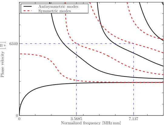
velocities are practically equal, both materials display significantly different values for their absolute nonlinearity parametersβ, which have been determined experimentally in [31]. Due to the marginal difference in the material properties that are required to define the dispersion curves, the same dispersion curves are used for the determination of possible cumulative second harmonic excitation setpoints for aluminum 6061–T6 and aluminum 1100–H14. Similar to the work of Deng, setpoints are identified for the symmetric mode pairs s1 → s2 and s2 → s4, which can be seen in Figure 3.1

and Figure 3.2, respectively. The numerical values for the frequencies and phase velocities associated with the two cumulative second harmonic excitation setpoints are summarized in Table 3.2. These values are determined based on dispersion curves that are calculated for a frequency normalized for a plate thickness of 1 mm. If plate thicknesses different from 1 mm are used, the fundamental and second harmonic frequency have to be scaled accordingly.

For the experimental work, the cumulative second harmonic excitation setpoint s1 →

s2 is examined. Experimental results for cumulative second harmonic generation at

(41)

0 0 3.5685 7.137 6349 Antisymmetric modes Symmetric modes Normalized frequency [MHz mm] P h a se v el o ci ty m s

Figure 3.1: Cumulative second harmonic excitation setpoint s1 →s2.

5.0832 10.1664 8078.9 Antisymmetric modes Symmetric modes Normalized frequency [MHz mm] P h a se v el o ci ty m s

(42)

Table 3.2: Two cumulative second harmonic excitation setpoints of aluminum 6061– T6 and aluminum 1100–H14 for a plate thickness of 1 mm.

setpoint fundamental frequency f1

second harmonic

frequency f2 phase velocity cph

s1 →s2 3.5685 MHz 7.1370 MHz 6349.0m_s

(43)

CHAPTER IV

EXPERIMENTAL PROCEDURE

This chapter presents all aspects of the experimental procedure. First of all, the Lamb wave generation via the wedge method is explained. Secondly, laser interferometry as a detection method is introduced. With the knowledge of Lamb wave generation and detection, in the subsequent section it is then possible to describe the experimental setup being disposed. Finally, an overview of the different specimens used in the experiments is given.

4.1 Generation of Lamb waves in plate specimens

Several methods are possible in order to launch a Lamb wave in a material speci-men. Examples are generation through a pulsing laser source, electromagnetic acous-tic transducers (EMATs), the comb transducer technique or the angle beam excita-tion [28], which is also referred to as wedge method. The wedge method is a very common technique and is used throughout all experiments for this work; it will be de-scribed subsequently. Additionally, details are given about the wedge design and the finalized wedge specifications for the cumulative second harmonic excitation setpoint s1 →s2 examined in this research.

4.1.1 Wedge method

For this method, a plexiglass wedge is used as a wave moderator between the ul-trasonic transducer and the specimen. The primary setup for the wedge method is depicted in Figure 4.1. It can be seen that the ultrasonic transducer is coupled to a wedge, which itself is coupled to the specimen. The wedge’s contact surface car-rying the transducer is inclined by an angle φcr relative to its contact surface with

(44)

the specimen. For proper acoustic coupling between the components, oil or glue are usually used. The ultrasonic transducer emits a longitudinal wave into the wedge,

Transducer φcr Wedge Specimen cLw clamb

Figure 4.1: Generation of a Lamb wave with the wedge method.

which propagates with the longitudinal wave speed cLw of the wedge material. The

longitudinal wave hits the boundary between wedge and specimen at the angle ofφcr.

This angle has to satisfy the Lamb wave excitation condition that can be derived from Snell’s law. For the interface between wedge and specimen, this condition is stated as

sin(φ2)cLw = sin(φcr)clamb, (4.1)

whereclamb is the velocity of the excited Lamb wave in the specimen and corresponds

to the chosen cumulative second harmonic excitation setpoint. Rearranging equa-tion (4.1) and incorporating that φ2 = 90◦ has to hold in order to launch a Lamb

wave leads to the following condition for the critical angle φcr in the wedge:

φcr = arcsin cLw clamb . (4.2)

By inspection it becomes clear that the longitudinal wave speed in the wedge has to be less or equal to the Lamb wave speed in the specimen for the critical angle condition to hold. Therefore, the wedge should always be made from a material with a relatively low longitudinal wave velocity, for instance plexiglass or polystyrene.

(45)

It has to be noted that in principle, only a single–directional and single–mode Lamb wave can be excited with the wedge method. While it might be a disadvantage for other purposes, this feature theoretically provides an advantage for this work, since all the energy transmitted at the generation side should be concentrated in one particular direction of propagation, leading to stronger signal amplitudes at the detection side. However, the experimental results in Chapter 6 show that due to the involved length scales the wedge still has to be considered as a point source. In general, if a multi– directional, multi–modal Lamb wave source is needed, a pulsing laser source is more appropriate.

4.1.2 Wedge design

In the work of Herrmann [12], several improvements for the wedge design are pro-posed. Their application is attempted for Lamb wave generation as well. In order to do so, the effect of beam divergence, which is also referred to as ultrasonic diffraction, has to be taken into consideration for the wedge design. Additionally, the attenua-tion of the wedge material plays an important role, since it weakens the Lamb wave launched in the specimen.

The effect of ultrasonic diffraction is caused by the fact that the ultrasonic transducer is not capable of launching a perfect plane longitudinal wave that remains within the imaginary cylinder below the cross–sectional area of the transducer. This is a result of diffraction in the wedge material. Therefore, some beams do not hit the interface between wedge and specimen at the critical angle. As a consequence, wave generation does not appear at the discrete desired phase velocity, but at a certain phase velocity spectrum. All additional phase velocities miss the Lamb mode to be excited, which is clear from the dispersion curves. Thus, in addition to the Lamb wave, bulk waves are generated, which carry a certain fraction of the energy that was intended exclusively for the Lamb wave.

(46)

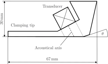
Additionally, the shape of the emitted beam magnitude possesses a Gaussian distri-bution, which means that the sound pressure has its maximum along the centerline of the transducer, the so–called acoustical axis, and decreases in radial direction. In order to compensate for these two effects, in [12] a modified wedge design is pro-posed for cleaner generation of Rayleigh waves. This design is used for Lamb wave generation as well and is shown in Figure 4.2. In contrast to the design proposed

θ Transducer Clamping tip Acoustical axis 67 mm 30 m m

Figure 4.2: Improved wedge design including a clamping tip (not to scale).

in [12], the wedge’s leading edge does not coincide with the point where the acous-tical axis hits the interface between wedge and specimen to minimize the effect of beam spreading. In fact, the wedge’s leading edge rather hits the point where the transducer’s leading edge hits that interface. Since the propagation distance in the wedge is significantly shorter for the Lamb wave measurements than for the Rayleigh wave measurements in [12] (due to a smaller critical angle of 25.85◦ _{for Lamb waves} compared to 64.5◦ _{for Rayleigh waves), the effect of beam spreading in the wedge} is much weaker. The results that are achieved with different wedge designs favor a design where the projection of the complete transducer cross–sectional area is used for wave transmission into the specimen, allowing more energy to be transmitted and

(47)

resulting in higher Lamb wave amplitudes.

However, in accordance to [12], a small additional incline θ and a rather voluminous region above that incline are created. This design makes sure that at least partially reflected beams off the acoustical axis do not reach the interface, but are manyfold reflected in the voluminous part of the wedge until they are sufficiently attenuated. Finally, it can also be seen that a rather long base has been added to the wedge. This base is used for clamping the wedge to the specimen. Although additional propaga-tion distance and hence attenuapropaga-tion is added for the longitudinal wave in the wedge, this has proven not to be problematic from a signal strength point of view. Even with the added thickness due to the clamping tip, the propagation distance in the wedge is shorter than in [12].

For the wedge material, a necessary condition is that the longitudinal wave speed in the wedge has to be smaller than that in the specimen in order to be able to fulfill the Lamb wave excitation condition. Once this condition is met, the preference is given to wedge materials with a low attenuation coefficient. Thus, the decrease of the signal strength due to attenuation is minimized. Feasible wedge materials are plexiglass and polystyrene. In Ginzel [10] and Herrmann [12], the longitudinal wave velocities and attenuation coefficients have been examined experimentally for these materials. The results show that for the excitation frequencies being used in this work, plexiglass displays a lower attenuation coefficient than polystyrene and is therefore the selected choice as a wedge material.

The critical angle in the wedge is determined according to Snell’s law, as previously described. With a longitudinal wave speed ofcLw = 2768.74m_s for plexiglass as wedge

material and a Lamb phase velocity of clamb = 6349m_s, the critical angle for the

cumulative second harmonic excitation setpoint s1 →s2 is calculated as

φcr = arcsin cLw clamb = arcsin 2768.74m_s 6349m_s = 25.85◦. (4.3)

(48)

For the acoustic coupling between ultrasonic transducer and plastic wedge, household glue of the brand Duco○R Cement is used. On the contrary, the acoustic coupling between wedge and specimen is ensured by the use of a light lubrication oil couplant, which is also used in [12].

4.2 Detection system

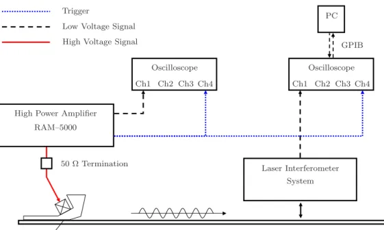
In order to be able to measure a relatively weak effect like the cumulative second harmonic in a propagating Lamb wave and moreover to measure simultaneously at two frequencies, a highly sensitive and broadband detection system is necessary. A good choice is in this case the single probe heterodyne laser interferometer, which has been previously described and used by Bruttomesso [2] and Hurlebaus [16, 17] and is depicted in Figure 4.3. The laser interferometer offers a variety of advantages:

Argon Laser 1 2–wave plate AOM Specimen Mirror 1 4–wave plate PBS Lens Photodiode NPBS Mirror vertical horizontal circular Polarization

Figure 4.3: Laser interferometer detection system.

• An absolute measurement of the out–of–plane surface velocity of the specimen can be performed.

(49)

• The laser measurement is made at a single point, thus being more precise than detection with a wedge–transducer combination.

• The broadband characteristic of the laser measurement makes it possible to measure multiple frequencies simultaneously.

• In contrast to the measurement with piezoelectric transducers, there is no me-chanical resonance involved, which makes a calibration dispensable.

• Since there is no physical contact between the laser system and the specimen, there is no interference or interaction of the measuring device with the effect to be measured. Moreover, a better repeatability is guaranteed due to the lack of a couplant and the associated difficulties (e.g. repeatability problems due to the thickness of the couplant layer).

Although there are also some disadvantages to the use of a laser interferometer system, they are mainly practical problems that can occur outside of a laboratory environ-ment. For instance, the alignment of the laser system and its sensitivity towards optical component vibrations can be problematic in field applications. Additionally, as a general requirement the specimen surface must be sufficiently reflective to the frequency of the laser light being used.

4.2.1 Doppler effect

The physical principle that is made use of by a laser interferometer is the well–known Doppler effect. In order to exploit this effect, first of all two beams of laser light are created that differ in frequency. They are referred to as object beam and reference beam. When the object beam hits the specimen surface and gets reflected off it, it is further influenced by the out–of–plane surface velocity of the specimen. This influence is again a frequency shift and is generally known as Doppler shift. After its reflection, the object beam is recombined with the reference beam, and analysis of

(50)

the resulting signal makes it possible to calculate the surface velocity which caused the frequency shift. According to the Doppler effect, the change in frequency ∆f is defined as

∆f = 2f v

c , (4.4)

wherevis the out–of–plane surface velocity of the specimen,f is the original frequency of the object beam, and cis the speed of light.

4.2.2 Acousto–optic modulator (AOM)

The acousto–optic modulator performs two basic functions for the laser interferome-ter: it splits a single laser beam into the object and reference beam, and it shifts the two exiting beams by a certain frequency. In the AOM, an incoming laser beam is split into multiple beams with the according frequencies fn =f +n·fb (n = 0...N),

where f is the frequency of the incoming beam and fb is the beat frequency of

the AOM. Additionally, the N + 1 outgoing laser beams are inclined by the an-gles θn = n·1.5◦ (n = 0...N). The first and second beam from the AOM, i.e. the

beams of order n = 0 and n = 1, carry already approximately 95 % of the energy of the incoming beam. Therefore these beams are very suitable as object and reference beams, respectively. If there is no out–of–plane surface velocity of the specimen, the beam stemming from the recombination of object and reference beam possesses a frequency f of the original laser signal, which is modulated by the beat frequency of the AOM, in this case fb = 40 MHz. Note, that the photodiode that detects the

recombined laser beam is only capable of detecting the modulating frequency in the incoming laser beam.