Optimization of Genomic Prediction of Single-Cross Performance in Maize
A DISSERTATION SUBMITTED TO THE FACULTY OF UNIVERSITY OF MINNESOTA
BY
Dnyaneshwar Chandrakant Kadam
IN PARTIAL FULFILLMENT OF THE REQUIREMENTS FOR THE DEGREE OF
DOCTOR OF PHILOSOPHY
Aaron J Lorenz, Advisor
i
Acknowledgements
I am foremost thankful to my advisor Dr. Aaron Lorenz for providing me the opportunity to work on this project and all his support and supervision throughout the course of this project. I am also thankful to my advisory committee at University of Minnesota, Dr. Candice Hirsch, Dr. Rex Bernardo and Dr. Shengqiang Zhong, and University of Nebraska, Dr. Ismail Dweikat, Dr. Stephen Kachman, and Dr. Thomas Hoegemeyer for their helpful suggestions and comments.
I am grateful to Indian Council of Agricultural Research for awarding me the fellowship for Ph.D. study, University of Nebraska and University of Minnesota for graduate education and necessary infrastructure for this project, Dr. Martin Bohn from University of Illinois for providing one dataset used in this research, and Dr. Ronald Haarmann from Pioneer for graciously allowing field experiments of hybrids at their York location for two consecutive years.
I would also like to thank Lorenz Lab members and friends for their help in this project as well as making my journey through graduate school pleasant.
Finally, I would like to express by gratitude to my family and relatives for their constant love and support throughout my education.
ii Abstract
Prediction of single-cross performance has been a major goal of plant breeders since the beginning of hybrid breeding because it is not feasible to evaluate all single-cross combinations between parental inbreds in a hybrid breeding program. Recently, simulation and experimental studies have shown great promise of genomic prediction of single-cross performance. However, further investigations are needed for optimal implementation of genomic prediction for single-cross performance. The objectives of this dissertation were to (1) examine the potential of genomic prediction of single crosses in the early stages of hybrid breeding pipeline, (2) evaluate the nonparametric models for genomic prediction of early-stage single crosses and (3) optimize the training set composition for genomic prediction of early-stage single crosses. Two different datasets consisting of 481 and 312 single crosses generated between random set of recombinant inbred lines (RILs)/doubled haploid lines (DHLs) derived from series of biparental families belonging to Iowa Stiff Stalk Synthetic (BSSS) and Non-Stiff Stalk Synthetic (NSSS) heterotic group were used. All the parental RILs/DHLs were genotyped using genotyping by sequencing approach. The accuracies of genomic prediction were substantially higher than topcross-based prediction commonly used in the early stages hybrid breeding. Moreover, genomic prediction outperformed phenotype-based prediction when only one or none of the parents of single crosses were tested. The mean genomic predictive abilities for T2, T1F, T1M, and T0 single crosses were 0.67, 0.60, 0.55, 0.46 for GY and 0.84, 0.74, 0.74, 0.63 for PH correspondingly. Genomic best linear unbiased prediction (GBLUP) and three nonparametric models namely reproducing
iii
kernel Hilbert space (RKHS), support vector regression (SVR) and neural network (NN) provided similar predictive abilities. Genetic relationship and training set (TRS) size in addition to the number of tested parents of single crosses considerably influenced the predictive abilities. Expected prediction accuracies based on prediction error variance (PEV) agreed well with empirical prediction accuracies when population structure was accounted. Genomic prediction models constructed on TRS optimized with PEV mean and coefficient of determination (CD) mean criteria provided increased predictive ability than stratified and randomly sampled TRS. Overall, the results of this study suggest that genomic prediction of early-stage single crosses with TRS optimization using PEV and CD mean criteria has great potential to redesign hybrid maize breeding and increase its efficiency.
iv Table of Contents
List of Tables ... viii
List of Figures ... xi
Chapter 1: Introduction and Literature Review... 1
INTRODUCTION ... 1
LITERATURE REVIEW ... 4
Hybrid Prediction Problem ... 4
Approaches for Hybrid Prediction ... 5
Genomic Selection ... 10
Comparison of Phenotypic, Marker Assisted Recurrent Selection and Genomic Selection ... 18
Genomic Selection for Hybrid Performance... 19
OBJECTIVES ... 23
Chapter 2: Genomic Prediction of Single Crosses in the Early Stages of a Maize Hybrid Breeding Pipeline ... 33
INTRODUCTION ... 34
MATERIALS AND METHODS ... 38
Germplasm ... 38
Field Experiments ... 39
Genotyping by Sequencing ... 40
Phenotypic Data Analysis ... 41
v
Cross-Validation and Prediction Accuracy Estimation ... 45
RESULTS ... 47
Variance Components and Broad-Sense Heritability ... 47
Prediction Accuracy for T2, T1F, T1M and T0 Scenarios ... 48
Prediction Accuracy for Novel Single-Cross Family ... 48
Genomic Predictions of Grain Yield of All Possible Single Crosses ... 49
DISCUSSION ... 49
Prediction Accuracy for T2, T1F, T1M and T0 Single Crosses ... 51
Comparison of Single-Cross Prediction Methods... 52
The Benefit of Modeling SCA ... 54
Prospects for Early-Stage Single-Cross Prediction... 55
Chapter 3: Evaluation of Nonparametric Models for Genomic Prediction of Early-Stage Single Crosses in Maize ... 65
INTRODUCTION ... 66
MATERIALS AND METHODS ... 71
Plant Materials and Field Experiments ... 71
Genotyping by Sequencing ... 73
Phenotypic Data Analysis ... 74
Genomic Prediction Models ... 76
RESULTS ... 85
Variance Components ... 85
vi
Phenotype and Genome-Based Predictive Abilities for T2, T1 and T0 Single Crosses
... 86
Influence of Tuning Parameters ... 87
Comparison of GBLUP and Nonparametric Models ... 88
DISCUSSION ... 89
Selection of Tuning Parameters ... 90
Comparison of GBLUP and Nonparametric Models for Single-Cross Performance Prediction ... 91
GBLUP vs Nonparametric Methods for Parent’s Combining Ability Based Prediction ... 93
GBLUP of Single-Cross Performance vs Combining Ability ... 95
Choice of Genomic Prediction Model for Single-Cross Performance ... 95
Chapter 4: Optimization of Training Set Composition for Genomic Prediction of Early-Stage Single Crosses in Maize ... 107
INTRODUCTION ... 108
MATERIALS AND METHODS:... 112
Germplasm ... 112
Genotyping by Sequencing ... 113
Phenotypic Data Analysis ... 114
Genomic Prediction Model ... 115
Cross-Validation Schemes ... 116
vii
Optimization Criteria and Algorithm ... 120
RESULTS ... 122
Variance Components and Heritabilities ... 122
Single-Cross Predictive Abilities with Different Levels of Relatedness ... 123
Comparisons of Expected and Empirical Prediction Accuracies ... 124
Comparisons of Training Set Optimization Methods ... 125
Training Set Optimization with All Possible Single Crosses ... 125
DISCUSSION ... 126
Effect of Different Levels of Relatedness on the Predictive Ability ... 126
Usefulness of Deterministic Formula to Design Training Set ... 128
Selection of Single-Cross Combinations for Phenotyping ... 130
Back to Shull’s “Pure Line Method of Corn Breeding” ... 131
Summary ... 141
Bibliography ... 145
viii
List of Tables
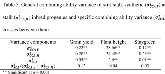
Table 1. Commonly used parametric and non-parametric models of genomic selection . 26 Table 2. Summary of published studies on genomic selection for per se performance, topcross performance and single-cross performance ... 28 Table 3. Family designations of nine single-cross families and number of single crosses belonging to each of the nine families. Biparental families are listed in the row and column headings. The numbers in the parentheses indicate numbers of recombinant inbred lines (RILs) or doubled haploid lines (DHLs) in the biparental family or number of single crosses in each single-cross family. Total number of single crosses per bi-parental family are displayed in the table margins. ... 57 Table 4. Mean, range, genetic variance and broad-sense heritability estimates in whole population as well as individual single-cross families for grain yield (GY; Mt/ha), plant height (PH; cm), and staygreen (SG; 1-10 rating) ... 58 Table 5. General combining ability variance of stiff stalk synthetic ( ) and non-stiff stalk ( ) inbred progenies and specific combining ability variance ( ) of single crosses between them. ... 59 Table 6. The parents of biparental families, number of RILs in each biparental family, number of single crosses for each of thirty six family wise cross combinations in dataset I. The total number of single crosses per biparental family are listed in the margins. ... 97 Table 7. The parents of biparental families, number of RILs in each biparental family, number of single crosses for each of nine family-wise cross combinations in dataset
ix
II. The total number of single crosses per biparental family are listed in the
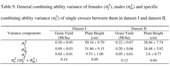
margins. ... 98 Table 8. Mean, range, variance components and heritabilities for grain yield (GY) and plant height (PH) in dataset I and dataset II. ... 99 Table 9. General combining ability variance of females ( ), males ( ) and specific combining ability variance ( ) of single crosses between them in dataset I and dataset II. ... 100 Table 10. Phenotype, topcross and genome based predictive abilities for grain yield (GY) and plant height (PH) in dataset I and II. ... 101 Table 11. Cross-validation based optimum values of tuning parameters of the three nonparametric methods RKHS, SVR and NN for grain yield (GY) and plant height (PH) in two datasets ... 102 Table 12. Predictive abilities of three nonparametric models obtained with optimum values of tuning parameters chosen by cross validations and default values
provided by respective software packages used to implement these models ... 103 Table 13. Correlation between observed and predicted GCA and SCA effects with GBLUP and three nonparametric methods RKHS, SVR and NN for grain yield (GY). ... 104 Table 14. Biparental families, number of RILs in each biparental family, number of single crosses for each of thirty six family-wise cross combinations. The total number of single crosses per biparental family are listed in the margins. The inbred groups denotes the classification of RILs based on realized genomic relationship.
x
... 133 Table 15. Mean, range, genetic variance ( ) and broad sense heritability ( ) estimates for whole population and nine groups of single crosses for grain yield (GY; Mt/Ha) and plant height (PH; cm) ... 134 Table 16. Mean expected prediction accuracies for grain yield with four training set (TRS) optimization methods when only 481 single crosses used and when all possible 9167 single crosses were considered. ... 135
xi
List of Figures
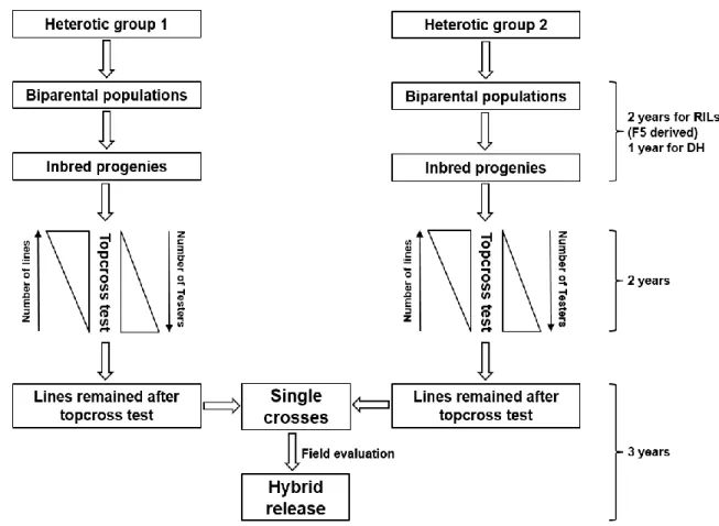
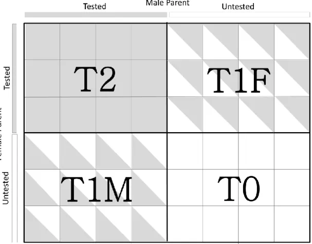
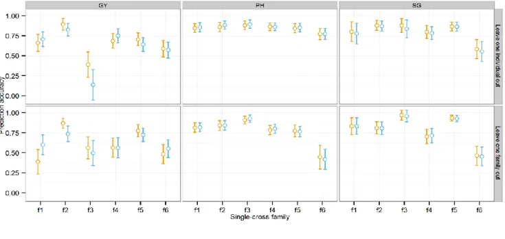
Figure 1. Schematic outline of typical hybrid maize breeding pipeline. Schematic outline of typical hybrid maize breeding pipeline. Estimated timeline for various stages adapted from Heffner et al., (2010) ... 31 Figure 2. Schematic outline of hybrid maize breeding pipeline with genomic selection. Estimated timeline for various stages adapted from Heffner et al., (2010). This scheme assumes the use of historical data for model training. ... 32 Figure 3. Crossing scheme between RILs or DHLs derived from three biparental families representing the SSS (y-axis) and NSS (x-axis) heterotic groups. Colored boxes indicate the presence while unfilled boxes indicate absence of a particular single cross. Bold lines delineate single-cross families... 60 Figure 4. Schematic visualization of T2, T1F, T1M and T0 cross-validation scenarios. Each small square represents one single cross. Completely filled squares (T2) indicate that both male and female parents of a single cross contained in the validation set were tested, half-filled squares indicate either the female (T1F) or male parent (T1M) of single cross contained in the validation set was tested, and unfilled squares (T0) indicate that neither parent of a single cross contained in the validation set was tested. ... 61 Figure 5. Prediction accuracy for T2, T1F, T1M and T0 cross-validation scenarios for traits grain yield (GY), plant height (PH) and staygreen (SG) obtained using the four methods 1a (Parent GCA), 1b (Parent GCA plus single-cross SCA), 2a (Additive genetic covariance among single crosses) and 2b (Additive plus
xii
dominance covariance among single crosses) as evaluated with training set of 250 and leave-one-individual-out cross-validation. ... 62 Figure 6. Mean prediction accuracy and standard errors of methods 1a (GCA) and 1b (GCA + SCA) in predicting performance of novel single-cross families. Two cross- validation schemes were used: leave-one-family out (bottom panel) and leave-one- individual out (top panel). Traits analyzed were grain yield (GY), plant height (PH), and stay green (SG). Standard errors were estimated using the bootstrap method... 63 Figure 7. Distribution of genomic predictions for grain yield (GY) for all 7866 possible single crosses between the 46 SSS inbred progenies and 171 NSS inbred progenies. ... 64 Figure 8. Single-cross predictive abilities based on phenotype (dashed lines) and four genome based methods GBLUP, RKHS, SVR and NN for T2, T1F, T1M and T0 single crosses for grain yield (GY) (A) and plant height (PH) (B) in dataset I and II as evaluated by leave-one-out cross-validation (LOOCV). ... 105 Figure 9. Effect of tuning parameters on the predictive ability of three nonparametric genomic prediction models. A: Effect of bandwidth parameter (h) on predictive ability of RKHS; B: Effect of ɛ-insensitivity, complexity parameter (C) and bandwidth parameter ( ) on predictive ability of SVR (Note: Only combinations providing predictive ability greater than 0.3 are shown to avoid overcrowding); C: Effect of number of neurons (s) on predictive ability of NN. Vertical planes (from left to right) represent 1. GY (dataset I), 2. PH (dataset I), 3. GY (dataset II) and 4.
xiii
PH (dataset II) ... 105 Figure 10. Realized genomic relationship among 10A. BSSS inbreds (females) and 10B. NSSS inbreds (males). GF1, GF2 and GF3 denote the three groups of inbreds based
on realized genomic relationship within BSSS and GM1, GM2 and GM3 denote the
three groups of inbreds based on realized genomic relationship within NSSS .... 136 Figure 11. Single-cross predictive abilities under different levels of relatedness between training set (TRS) and test set (TS). 11A.Leave-one-group cross-validation scheme used. GF1, GF2 and GF3 denotes three BSSS inbreds groups and GM1, GM2 and GM3 denotes three NSSS inbred groups based on realized genomic relationships. G2-Both parents of validation group of single crosses (SC) were tested, G1-Either male or female parents of validation group of SC were tested. Letters W, C, and D denotes SC from validation group, closely related group and distantly related group respectively. 11B. Predictive abilities for grain yield (GY) and PH for different TRS compositions using GCA or GCA and SCA ... 137 Figure 12. Expected Vs Empirical predictive ability for training set compositions D, C+D, C and across population (R). Without accounting for population structure 12A. Grain yield, 12B. Plant height. With accounting for population structure 12C. Grain yield, 12D. Plant height ... 138 Figure 13. Predictive abilities of model constructed using optimized training set selected out of 481 single crosses based on PEVmean, CDmean, stratified sampling and random sampling. 13A. Grain yield (GY), 13B. Plant height (PH)... 139 Figure 14. Prediction error variance (PEV) of model constructed using optimized training
xiv
set selected based on PEVmean, CDmean, stratified sampling and random
sampling. 14A. TRS optimization out of 481 single crosses 14B. TRS optimization out of all possible 9167 single crosses ... 140
1
Chapter 1: Introduction and Literature Review
INTRODUCTION
Maize is one of the most important cereal crop worldwide (Shiferaw et al. 2011). It belongs to grass family Poaceae (Gramineae) which also includes other major cereals such as wheat and rice. Maize is further classified into genus Zea, a group of annual and perennial grasses native to Mexico and Central America. The genus Zea comprises wild taxa, collectively known as teosinte (Zea spp.) and domesticated maize (Zea mays L. ssp.
mays). Genetic studies have indicated that maize is domesticated directly from Mexican annual teosinte Zea mays ssp. parviglumis, native to the Balas river valley in south-eastern Mexico (Matsuoka et al. 2002). Maize being a versatile crop is grown over a wide range of agro climatic zones (Hake and Ross-Ibarra 2015). The United States, China, Brazil are the top three maize producing countries in the world. Important uses of maize include food, animal feed and bioenergy production (Ranum et al. 2014). Maize is also an exciting model organism for biological research including plant domestication, genome evolution, epigenetics, heterosis and quantitative inheritance (Strable and Scanlon 2009).
Development of hybrid maize is one of the landmark achievement in the history of plant breeding (Duvick 2001). Shull (1908, 1909, 1952) first proposed a method for exploitation of heterosis through the development of single-cross hybrid. His method consist of two steps. In the first step, pure line are developed by self-fertilization and the second step consist of identification superior hybrid combination among the pure lines.
2
This method is referred as “pure line method of corn breeding”. Although Shull’s method has become a standard procedure hybrid breeding programs, several modifications have occurred over the past hundred years to efficiently generate lines and identify superior hybrid combination between them. The main modifications include organization of inbreds into heterotic groups to increase the probability of obtaining superior hybrids (Reif et al. 2005), population improvement methods to increase the frequency of lines having good potential for hybrid performance (Comstock et al. 1949), topcross test-based screening of lines for hybrid performance (Jenkins and Brunson 1932), doubled haploid (DH) technology to rapidly generate homozygous lines (Rober et al. 2005).
Contemporary hybrid maize development program consist of two overlapping stages 1) line development and 2) hybrid evaluation (Figure 1). Development of lines is most commonly carried out by selfing in a pedigree breeding method or DH technology. The crosses between elite lines in each heterotic group are typically used to derive recombinant inbred lines (RILs) or DH lines (DHLs) (Bauman 1982; Mikel and Dudley 2006). Prior knowledge of performance of parental lines in earlier breeding cycles and pedigree relationships is used to determine the potential of specific cross. Simulation studies indicate that selection of parents of crosses is far more important than number of crosses and number of lines within each cross (Bernardo 2003; Wegenast et al. 2008). For RILs development via pedigree method, selection and selfing is initiated in F2 population without any genetic recombination as the effects of random mating in F2 population before selfing are not conclusive (Bernardo 2002). DHLs are typically produced from F1 plants instead of F2 plants to shorten the length of breeding cycle
3
(Longin et al. 2007). Recent studies, however, suggest to produce DHLs from F2 plants preferably after selecting for disease and insect resistance, marker associated traits or topcross performance (Wegenast et al. 2008; Bernardo 2009).
Characterization and selection of lines involves sequential testing. Initially lines are selected based on per se performance and topcross test while selections in the advanced stages are performed by general combining ability (GCA) and specific combining ability (SCA) evaluation in hybrid combinations. The selections based on per se performance is carried out for traits having reasonably high heritability and are considered necessary for hybrid performance such as maturity, plant canopy architecture, ear size, grain quality and resistance to certain pests and diseases. In case of RILs development, topcross testing is commonly performed in F3 and F4 generations after the lines having poor per se performance are discarded (Hallauer and Miranda 1988). Similarly, only those DHLs having suitable per se performance are evaluated in topcross test. Typically, two generations of topcross testing are conducted (Heffner et al. 2010). With each round of topcross test, the number of lines advanced decreases while number of testers used increases. Narrow-based testers such as elite inbred from opposite heterotic group are commonly used for topcross test. Theoretical and empirical results shows that elite inbred from opposite heterotic group generate testcross genetic variability as large as when poor performing tester is used (Hallauer and Lopez-Perez 1979; Bernardo 2002). Additionally, they are more practical because superior hybrid combination can be commercialized in a short period of time.
4
Lines selected based on topcross performance are evaluated for GCA and SCA in hybrid combinations. Lines retained after GCA and SCA testing are further evaluated in more hybrid combinations at multiple locations. Resources are allocated to evaluate as many lines as possible at topcross stage with intense selection, while at later stages, emphasis is placed on testing fewer hybrid combinations at many locations. The RILs/DHLs with superior GCA and stability identified from multilocation hybrid evaluation are often recycled as parents to develop source populations for line development (Smith 2004). A typical structure of commercial hybrid maize breeding program based on DHLs is depicted in Bernardo (2002).
LITERATURE REVIEW
Hybrid Prediction Problem
Currently, heterotic groups are well established in maize and single-cross hybrids are exclusively made by crossing RILs/DHLs across heterotic groups (Reif et al. 2005). This greatly facilitates the hybrid development. However, as the number of lines to be tested are increasing over time especially with advances in DH technology, their evaluation in all possible hybrid combination is challenging. For example, if the breeder has just 100 RILs/DHLs in each heterotic group, the total number of hybrid combination to evaluate is 10,000. Therefore, evaluation of lines for hybrid performance has been the most expensive and critical phase in hybrid maize breeding. If the promising single crosses could be identified without the need to generate and test several thousand
5
possible single-cross combinations, the efficiency of hybrid breeding would be greatly enhanced (Schrag et al. 2009).
Approaches for Hybrid Prediction
In view of its potential to accelerate the hybrid breeding, prediction of hybrid performance has been the major goal of numerous studies. Below is the brief description of different approaches investigated for hybrid prediction.
Inbred per se performance
The possibility of inbred per se performance as indicative of its performance in hybrid combination is desirable to reduce the number of hybrid combinations to be made and tested. Many correlation studies between inbred and hybrid traits were undertaken in the past. The results of these studies were summarized in Hallauer and Miranda (1988). The correlations between inbred per se performance and hybrid performance were variable depending on the traits considered, environment, and tester used. In general, the correlations were relatively high for simple traits such as morphology, ear traits, maturity, quality characters etc. but were relatively low for complex trait such as grain yield. The poor correlations between inbred and hybrid grain yield were due to presence of strong nonadditive effects (Hallauer 1990) and genotype by environment interaction for this trait (Bernardo 1991). Environmental factors also influence the correlation between inbred and hybrid traits. Betran et al. (2003) found stronger correlation between inbred and hybrid traits under severe drought stress than under unstressed environments. Smith (1986) reported low theoretical correlation between inbred per se performance and
6
testcross performance for traits controlled by large number of genes showing complete dominance. The type of tester influenced this correlation, the correlations were low but greater with good unrelated tester than with a good related tester. It is now generally agreed that effective selection can be made on inbred per se performance for certain traits, but evaluation in hybrid combinations is required to identify the lines with best breeding values for complex traits (Hallauer and Miranda 1988).
General combining ability
Combining ability is defined as the capacity of individual to inherit superior performance to its offspring. Initially, it was a general concept used for classifying the lines relative to its performance in hybrid combinations. Sprague and Tatum (1942) refined the concept of combining ability into GCA and SCA. They defined GCA as the average performance of line in a series of hybrid combinations and, SCA as those instances in which certain hybrid combinations are either better or poorer than would be expected on the basis of average performance of parental lines included. Generally, GCA is considered to be an indicator of additive genetic effects, while SCA is related to the nonadditive genetic effects.
Several techniques have been proposed for the estimation of combining ability (Fasahat et al. 2016). The two main techniques include topcross test suggested by Davis (1927) and developed by Jenkins and Brunson (1932) and diallel analysis by Griffing (1956). Evaluation in diallel schemes is ideal as it provides information of both GCA and SCA. However, number of single crosses required for diallel analysis inceases
7
exponentially with increase in the number of lines. Therefore, diallel cannot be conducted practically with substantial number of lines. When the lines belongs to distinct groups like heterotic groups in maize, combining ability evaluation is performed in two factor factorial design (Comstock and Robinson 1948). Analysis of factorial can also provide information on both GCA and SCA. However, as with diallel, it is difficult to evaluate large number of lines in complete factorial because total number of crosses becomes unmanageable.
Topcrossing with appropriate tester has been a simple and widely used approach to evaluate the combining ability of lines (Jenkins and Brunson 1932). The tester genotypes can be classified into two groups namely broad genetic base tester (e.g. Synthetic variety) and narrow genetic base tester (inbred and single-cross hybrid). A broad genetic base tester is considered for GCA evaluation while narrow genetic base tester is useful for SCA evaluation. The average performance of lines with more than one inbred tester is also considered as the measure of lines GCA.
The sum of parental lines GCA estimated using performance in hybrid combinations or topcross test is a simple and established approach to predict single-cross performance (Cockerham 1967; Melchinger et al. 1987). The correlations between parents GCA and single-cross performance ranged from 0.68 - 0.94 in different experimental studies in maize (Schrag et al. 2006, 2007). Topcross based screening of lines has limitation that it takes longer time to develop commercial hybrid due to additional years of topcross test. Also, all possible single-cross combinations among
8
available lines cannot be evaluated due to discarding of lines based on topcross test which could include some potential hybrids.
Best linear unbiased prediction
Best linear unbiased prediction (BLUP) is used in linear mixed model for the estimation of random effects. BLUP was derived by C. R. Henderson for the prediction of breeding values in animal breeding (Henderson 1984). Bernardo (1994, 1995, 1996a, 1996b) showed the usefulness of BLUP with interpopulation genetic models involving both GCA and SCA for prediction of untested single crosses. The BLUP approach for single-cross performance used information on genetic relationships among the parental lines, based on coefficient of coancestry estimated from pedigree or molecular marker data. Later, Bernardo (1998) extended aforementioned BLUP (T-BLUP) approach to make use of both trait and marker data (TM-BLUP). In TM-BLUP approach, covariances associated with quantitative trait loci (QTLs) were modelled by inferring the identity by descent of unobservable QTLs from flanking markers. In experimental study, however, T-BLUP and TM-BLUP resulted in similar prediction accuracies which was explained by presence of large number of QTLs for grain yield (Bernardo 1999b). Results indicated that BLUP is useful for routine prediction of single-cross performance (Bernardo 1999a). Pedigree-based BLUP, however, has limitation that it is ineffective in comparing inbreds developed from single biparental population, as they possess the same pedigree (Bernardo 2002). Also, pedigree information is not always available in the breeding program, and, when available does not always have high reliability. The hybrid
9
prediction accuracies of marker based BLUP could be further improved by use of genome wide dense marker data available in the recent years (Xu et al. 2014).
Genetic distances based on molecular markers
With the discovery of molecular markers, genetic distances (GD) between parental lines based on random DNA markers were tested for predicting hybrid performance. Quantitative genetics theory suggests that the amount of heterosis is a function of the allelic diversity between two parents (Falconer et al. 1996). Therefore, GD based on molecular markers seemed to be a logical approach for prediction of hybrid performance. However, correlations between hybrid performance and GD for inter-heterotic group hybrids have been very low and/or inconsistent (Melchinger 1999; Lee et al. 2007). Two possible sources of these low prediction accuracies include (1) loose linkage between heterotic QTL and the molecular markers used to estimate GD and (2) opposite linkage phases between the QTL and marker alleles as generally expected with inter-heterotic group hybrids (Charcosset et al. 1991; Bernardo 1992). Commercial hybrids in maize consist of only inter-heterotic group single crosses, making them the only ones relevant for prediction in breeding programs.
Hybrid performance associated markers
In a modified approach, molecular markers were first tested for association with hybrid traits. Subsequently, a sum of the effects of significantly associated markers (“total sum of selected markers TCSM”) was used for prediction of hybrid performance and SCA (Vuylsteke et al. 2000). However, this approach was found to be less effective
10
than established GCA method (Schrag et al. 2006). Further, Schrag et al. (2007) extended TCSM approach to account for the multiple testing, missing marker data, multiple alleles, which they referred as “total effects of associated markers” (TEAM). The prediction accuracies were still substantially lower than GCA method. Also, extending the GCA predictions with SCA estimates from associated markers did not improve the prediction accuracy (Schrag et al. 2006).
Genomic Selection
Genomic selection (GS) is defined as the selection for a trait of interest using large number of genomewide markers (Meuwissen et al. 2001). The main difference between marker assisted selection (MAS) and GS is that only the markers that are significantly associated with QTL are used in MAS, while all the markers are used simultaneously without significance testing in GS. An implicit assumption in GS is that all QTLs are in LD with at least one marker. GS has become feasible in the recent years because of following advances in the science and technology: 1. Efficient methods to genotype large number of SNPs discovered by whole genome sequencing (Thomson 2014), 2. Successful application of statistical methods to handle the high dimensional marker data (Gianola et al. 2010; de los Campos et al. 2013), and 3. Availability of high capacity computational resources (Wu et al. 2011). GS is expected to be more effective than MAS especially for traits controlled by many small effect QTLs because the marker effects are less biased in GS compared to MAS as all the marker effects are estimated simultaneously. Also, the proportion of genetic variance explained by markers is larger in
11
GS than MAS as small effect QTLs that do not meet the significance threshold are missed in MAS (Jannink et al. 2010).
The central process of GS consist of two steps. First step is the construction of genomic prediction equation by using marker and phenotypic data on the subset of individuals called the training set (TRS). Second step consist of using the prediction equation to calculate genomic estimated breeding value (GEBV) for a set of selection candidates having only marker data called test set (TS) and then to select the best candidates based on their GEBV. The main challenge in building a genomic prediction model is that number of molecular markers (i.e. predictors) is typically far more than number of individuals in the TRS (i.e. observations) known as “large p and small n”
problem. In this situation, ordinary least square estimates of parameters have large variances leading to poor predictive ability. To confront this problem, a slew of alternative statistical models have been employed with different underlying assumptions. These models can be broadly separated into two categories: parametric and non-parametric. Prominent features of different parametric and nonparametric GS models as well as software packages used to implement them are provided in Table 1. Briefly, parametric models on priori assume a certain form relationship between genetic value and marker covariates. The marker effects are estimated either using shrinkage or combination of shrinkage and variable selection procedure. The common parametric models include ridge regression best linear unbiased prediction (RRBLUP) and Bayesian models. In RRBLUP, marker effects are assumed to be random and normally distributed with common variance resulting in equal shrinkage of their effects. The RRBLUP model
12
can be implemented in mathematically equivalent but computationally efficient form GBLUP (Habier et al. 2007). GBLUP uses genomic relationship matrix (GRM) derived from marker genotypes among the individuals (VanRaden 2008) instead of calculating individual marker effects. This reduces the number of equations required to be solved from p to n. In contrast to RRBLUP, Bayesian models fits marker specific variances resulting in unequal shrinkage of their effects. Bayes A assign t-distribution for marker effects which causes strong shrinkage towards zero for small estimates of marker effects and less shrinkage for sizable estimates of marker effects. Bayes B also assign t -distribution for marker effects but, additionally, can set large number of marker effects to zero. Bayes C method is similar to Bayes B except that it assign normal distribution to nonzero marker effects.
Non-parametric models take a different approach by not making strong assumption about the form of relationship between markers and genetic value. Instead, these models seek the form that best fits in TRS data while maintaining some generality for new data. In another words, their main focus is on prediction. These models are, therefore, expected to capture nonaddtive effects without explicitly modelling them and provide better prediction of phenotypes for complex traits (Gianola et al. 2006, 2010). Some commonly used nonparametric GS models include reproducing kernel Hilbert spaces (RKHS), support vector regression (SVR) and neural network (NN). RKHS model uses kernel function to define the genetic relationship between individuals which enables to perform non-linear regression in high dimensional feature space. SVR and NN are
13
machine learning methods which are used to address large p small n problem in many field.
The predictive performance of GS models is typically evaluated by cross-validation (CV) technique. CV is applied in a number ways depending on the specific objective of the study. CV design includes 1. k-fold validation, 2. Repeated random sampling validation, 3. Across cycles/generations validation, 4. Across populations validation, and 5. Across environments validation. In k-fold CV, the entire data set is randomly divided into k folds. Out of which, k-1 folds are used to train the GS model and remaining fold is used as TS. The procedure is repeated till each fold is included in the TS one time. Repeated random sampling CV involves random sampling of data into TRS (e.g. 90 percent) and TS (e.g. 10 percent) several times. Other CV designs (i.e. 3,4,5) involves stratification across cycles/generations, populations, environments correspondingly.
The accurate assessment of prediction accuracy is an important component in evaluating predictive performance of different models. Ideally, the accuracy of GS is the correlation between true breeding value (TBV) and GEBV. However, in practice, TBV is unknown. Considering cor ( , y) = cor ( , ) × cor ( , ), where y is vector of phenotypes; is a GEBV and is TBV, the prediction accuracy is estimated as cor ( , y) / h because h2 (heritability) = (cor ( , ))2 (Legarra et al. 2008; Hayes et al. 2009).
GS accuracy is affected by several factors acting interconnectedly. These factors mainly include genetic relationship, heritability, TRS size, marker density and statistical
14
methods. Below we describe the connection between individual factor and the prediction accuracy. A detailed discussion of the effects of different factors on GS accuracy can be found in Lorenz et al. (2011) and Lin et al. (2014).
Genetic relationship
The genetic relationship between TRS and TS is the most important factor influencing the accuracy of genomic prediction. The TRS needs to representative (i.e. closely related) to the TS in order to get good prediction accuracy. The closer genetic relationship benefits the prediction accuracy in two ways 1. It reduces the effective population size generating strong long range linkage disequilibrium (LD) between maker and QTL, and 2. Estimated marker effects are well predictive in TS due to related genome structure. The prediction accuracy is, therefore expected to be highest for training and prediction within population (full sib relationship), followed by populations connected by one shared parents (Half sib relationship). Empirical GS studies in many crops including maize have stressed the importance of genetic relationship for obtaining good prediction accuracy (Albrecht et al. 2011; Riedelsheimer et al. 2013; Jacobson et al.
2014; Albrecht et al. 2014).
Heritability
Heritability is an important determinant of achievable prediction accuracy. High heritability enables to estimate marker effects accurately because phenotypic variation is mostly composed of genetic variation with only little confounding effect of environmental factors. Highly significant correlation has been observed between
15
heritability and prediction accuracy in empirical studies in maize (Lorenzana and Bernardo 2009; Jacobson et al. 2014). Although the accuracy of both GS and phenotypic selection is affected by heritability, GS becomes more efficient over phenotypic selection with decrease in heritability (Bernardo and Yu 2007; Viana et al. 2016). The genetic relationship information and LD between markers and QTLs enable GS to outperform the phenotypic selection under low heritability situation.
Training Set size
Increasing the TRS size allows accurate estimation of marker effects and consequently enhance the prediction accuracy. Positive correlation between TRS size and prediction accuracy has been reported from studies in maize (Lorenzana and Bernardo 2009; Albrecht et al. 2011; Zhao et al. 2012). The empirical studies in maize indicate that minimum TRS size of about 50 -100 when predicting within a biparental population (full sib) (Lorenzana and Bernardo 2009; Albrecht et al. 2011; Riedelsheimer et al. 2013) and about 300 - 400 when predicting for populations related by at least one common parent (half sib) (Zhao et al. 2012) are required to obtain prediction accuracy above 0.5 assuming moderate to high heritability. It is important to note that increasing the genetic relationship between TRS and TS is more effective way to increase the prediction accuracy than increasing the TRS size by adding less related individuals. Alternatively, reasonable TRS size is required to obtain reliable prediction even under close genetic relationship between TRS and TS.
16
The number of markers required to obtain optimal prediction accuracy depends on LD in the population under consideration. If the LD is high, less markers are required and vice versa. The prediction accuracy benefits from increasing the number of markers until sufficient genome coverage is attained. Also, increasing marker density is beneficial only with corresponding increase in TRS size. In maize, about 100 markers for GS within biparental population and 200 - 400 markers for GS with multiple interconnected populations are suggested to get optimal prediction accuracy (Lorenzana and Bernardo 2009; Zhao et al. 2012). Due to readily availability of cheap and abundant genome wide SNPs now a days, marker density would not be limiting factor to obtain maximum achievable prediction accuracy. Type of markers used can also influence the prediction accuracy. Solberg et al. (2008) reported that three times higher SNP density is required to obtain prediction accuracies comparable to SSR. This is because SSR have multiple alleles and therefore contain more information. The multi-allelic system of SSR can be mimicked by constructing haplotype containing multiple alleles. The improvement in prediction accuracy using haplotype is however minimal especially when SNP density is high (Calus et al. 2008). In another study, Poland et al. (2012) found greater GS accuracy using SNPs obtained from GBS than DArT marker.
Statistical model
The prediction accuracy of different GS models depends on genetic architecture of the trait and LD structure in the population. Simulation results indicate that RRBLUP and GBLUP rely strongly on kinship while Bayesian models focus more on LD between
17
marker and QTL than on kinship (Habier et al. 2007; Zhong et al. 2009). Thus, if there are only few major effect QTLs for a trait, Bayesian models can provide better accuracy over RRBLUP and GBLUP. Alternatively, if there are many small effect QTLs both methods can achieve similar prediction accuracies. The results of empirical studies, however, showed comparable performance of both types methods across different types of trait architectures (Lorenzana and Bernardo 2009; Moser et al. 2009). When strong long range LD exist in a population, the effects of major QTLs can be captured by markers well apart from the QTL (i.e. distribution of QTL effect) resulting in good prediction accuracies of RRBLUP. When the nonadditive gene effects are important for a given trait, simulation and some experimental studies indicate the better performance of nonparametric models over parametric methods (Heslot et al. 2012; Pérez-Rodríguez et al. 2012; Howard et al. 2014; Jiang and Reif 2015).
One of the key issue in implementing the GS in a breeding program is how to design TRS to obtain optimal prediction accuracy with minimum phenotyping. One of the approach would be to use phenotypic and genotypic data on genetically related individuals for model calibration. Typically, several lines are evaluated very year in a breeding program. Hence, the phenotypic and genotypic data from multiple differentially related populations is likely to be available even before a new cross is made. Selective phenotyping is another important alternative to reduce the phenotyping expenses involved in GS. Here, the objective is to select minimum number of individuals that are best suited to build the genomic prediction model. Some of the criteria for selection of individuals include stratified sampling, minimizing the prediction error variance (PEV)
18
and maximizing the reliability (i.e. coefficient of determination) (Rincent et al. 2012; Isidro et al. 2015).
Comparison of Phenotypic, Marker Assisted Recurrent Selection and Genomic Selection
The relative efficiencies of phenotypic selection, marker assisted recurrent selection (MARS) and GS were compared in simulation and experimental studies in maize. Bernardo and Yu (2007) first showed the effectiveness of GS in plant breeding. They simulated MARS and GS for testcross performance using DHLs derived from single biparental population. The response to GS was 18 to 43% larger than MARS across different numbers of QTLs and levels of heritability. Later, Massman, et al.
(2013b) provided the first empirical proof of advantage of GS over MARS in crops. Their experiment involved two cycles of GS and MARS for testcross performance for stover and yield indices in a population consisting of 233 RILs derived from B73 and Mo17. The realized gains were 14 to 50% larger with GS compared to MARS. Further, Beyene
et al. (2015) compared the genetic gain for grain yield in eight biparetal populations under managed drought stress conditions using GS vs pedigree selection. The response to GS was two to four times higher than pedigree selection. The average gain from GS per cycle across eight populations was 0.086 Mg ha-1. They also reported that hybrids derived from cycle 3 (C3) produced 7.3% higher grain yield than those developed through pedigree breeding. Recently, Vivek et al. (2017) reported a study on genetic gain under drought conditions using phenotypic selection and GS in two biparental populations. C1
19
was formed by intermating the top 10% families selected based on testcross performance. Subsequently, C2 derived based on phenotypic selection (C2-PS) and GS (C2-GS). Topcrosses of C2-GS showed 4 - 43% higher grain yield than those of C2-PS. In another recent study, Zhang et al. (2017) first applied rapid cycle GS to multiparental population derived from 10 elite maize parents for four recombination cycles. The realized genetic gain with GS cycles (C1-C4) was 0.225 tonn ha-1 cycle-1 which is equivalent to 0.100 tonn ha-1 year-1.
Genomic Selection for Hybrid Performance
Several studies have examined the potential of GS at different stages of hybrid maize breeding including per se performance, topcross performance, and single-cross performance (Table 2). GS for per se performance of lines has limited usefulness as the value of line in hybrid breeding is determined by its performance in hybrid combination. However, GS can be benefical for traits such as disease resistance which are evaluated on line per se. Technow et al. (2013) investigated the accuracies of genomic prediction of northern corn leaf blight resistance among inbreds belonging to dent and flint heterotic group. The prediction accuracies were low to moderate. They found considerable benefit of increasing the training set size within heterotic groups as well as by combining inbreds across two heterotic groups. Riedelsheimer et al. (2013) evaluated the prospects of combining multiple differently related populations into TRS for predicting per se performance of lines for five traits including Gibberella ear rot severity and three kernel yield component traits. They observed considerable decline in predictive ability when full
20
sib lines were replaced by half-sib lines, but significant predictive abilities were obtained when half-sib lines were available from both the parents instead of only one parent of validation population. Also, some negative effect of combining unrelated populations into TRS was observed.
The genomic prediction studies for topcross performance have looked at the effect of different factors such as TRS size, marker density, prediction within vs across populations, prediction across testers. Generally, the topcross prediction accuracies were benefited by increase in TRS size and number of markers (Lorenzana and Bernardo 2009; Albrecht et al. 2011; Zhao et al. 2012). Prediction within a biparental population is an ideal scenario because of close relationship between TRS and TS and long range haplotype blocks which creates high LD between marker and QTL. As expected, the mean topcross prediction accuracies for within biparental population were moderate to high (Lorenzana and Bernardo 2009; Albrecht et al. 2011; Zhao et al. 2012). However, in this scenario, there is the need to phenotype a subset of individuals from the same population which increases the time and cost before genomic prediction can be performed. Also, individual population sizes need to be sufficiently large to reliably perform within population predictions (Schulz-Streeck et al. 2012). It would therefore be advantageous if performance of lines within a biparental population could be predicted before that population is phenotyped. In this context, some studies investigated the effect of estimating marker effects across populations to predict within each population (Albrecht et al. 2011; Zhao et al. 2012; Jacobson et al. 2014). The prediction accuracies were similar or slightly lower than within population prediction when the topcross
21
information of half-sib lines from both the parents were available. The prediction accuracies were severely decreased when topcross information of half-sib lines from only one or none of the parent were available. Furthermore, when the diversity panel was used to estimate the marker effects, the prediction accuracies were negatively affected (Windhausen et al. 2012). Few possible reasons for decrease in accuracy of genomic prediction for across-within scenario include marker x population interaction, epistasis and different linkage phases between maker and QTL among populations (Schulz-Streeck
et al. 2012). In an effort to enhance prediction accuracy, models including population specific marker effects (Schulz-Streeck et al. 2012) or only the preselected markers having low marker x genetic background interaction (Zhao et al. 2012) were investigated. However, no improvement in the prediction accuracy was observed. In a different scenario, when the estimation and prediction were performed across the bi-parental populations, the prediction accuracies were higher compared to within biparental population prediction (Albrecht et al. 2011; Schulz-Streeck et al. 2012; Zhao et al. 2012; Windhausen et al. 2012). The increase in prediction accuracy resulted from differences in mean performances of populations rather than kinship between estimation and prediction set and LD between markers and QTLs (Windhausen et al. 2012). As genetic variation among populations can be efficiently exploited through parental selection, GS application is not needed in this scenario. Albrecht et al. (2014) explored the possibility of topcross prediction across testers wherein disappointingly low accuracies were observed.
The prospects of GS for single-cross performance have been investigated with simulation and experimental studies in maize (Technow et al. 2012; Massman, et al.
22
2013a; Technow et al. 2014). All the studies reported high accuracies of genomic prediction of single crosses. Increasing the number of tested parents (0, 1, 2) (Technow et al. 2012; Massman, et al. 2013a; Technow et al. 2014) as well as increasing the number of single crosses per tested parent (Technow et al. 2014) significantly improved the prediction accuracies. Also, Technow et al. (2012) found small benefit of increasing the marker density and modelling population specific marker effects and dominance in the prediction model. The accuracies of GBLUP and Bayes B were very similar (Technow et al. 2014). In a comparison of genome and transcriptome-based single cross prediction, Zenke-Philippi et al. (2016) observed similar prediction accuracies of ridge regression model employing these two different type of markers.
The potential of genomic prediction of single-cross performance was also studied in other crops including wheat and rice in which moderate to high accuracies were observed. In a wheat dataset consisting of 90 single crosses derived from 22 females and 13 males elite lines, Zhao et al. (2013) investigated the predictive performances of RR-BLUP, Bayes A, Bayes B, Bayes C and Bayes C models incorporating additive and dominance marker effects. The prediction accuracies were high (0.58-0.63) for all the models with slight superiority of RR-BLUP and Bayes B. In their study, ignoring the dominance effect resulted in equal or slightly higher prediction accuracies. In another largest experimental study in wheat, Zhao et al. (2015) performed genome and metabolite-based prediction of single-cross performance using 1604 single crosses generated by crossing 120 diverse female and 15 male lines. The mean genome-based prediction accuracies were 0.89 for T2 single crosses, 0.65 for T1 single crosses and 0.32
23
for T0 single crosses. They found no improvement in the prediction accuracy with either modelling epistasis or metabolite profiling. Xu et al. (2014) compared GBLUP, Bayes B and LASSO for predicting single-cross performance in rice. They used 278 single crosses generated between 210 RILs derived from single biparental population. All the three methods provided similar results. The predictabilities (squared correlation between observed and predicted values) for grain yield, number of tillers per plant, number of grain per panicle and 1000 grain weight were ranged from 0.09-0.16, 0.20-0.23, 0.35-0.37 and 0.67-0.69 respectively. Further, they found no noticeable improvement in prediction accuracy by including dominance and epistatic effects in GBLUP model.
OBJECTIVES
As described in the introduction, the early stages of hybrid breeding consist of generation of RILs or DHLs from several biparental population for evaluation in hybrid performance. The initial selection of lines is based on per se performance and topcross test using one or multiple testers and evaluation in single-cross combinations is delayed until advanced stages. This process has the advantage that lines having poor potential for hybrid performance are discarded in the early stages which allows concentration of resources on more promising lines. In accordance with this process of commercial hybrid development, published genomic hybrid prediction studies have investigated the potential of genomic prediction for topcross performance using the experimental material resembling to the early stages (Lorenzana and Bernardo 2009; Albrecht et al. 2011; Zhao
24
material resembling to advanced stages of hybrid breeding (Massman, et al. 2013a; Technow et al. 2014). The current procedure of hybrid development, however, has some limitations which include more time for commercial hybrid development due to additional generations of topcross testing and inability to evaluate all possible single-cross combinations among the available lines which leaves open the possibility for losing some unique potential single crosses. Therefore, it would be desirable to investigate the potential of genomic prediction of single crosses in the early stages of hybrid development (Figure 2).
Also, published studies on genomic prediction of single-cross performance have mainly used parametric models such as GBLUP and Bayes A, Bayes B, Bayes C and Bayes C . The parametric models make on a priori assumptions about the form of relationship between markers and genotypic value. These assumptions often do not hold in typical breeding populations limiting the ability of these models to precisely capture nonaddtive genetic effects (Gianola et al. 2006; Howard et al. 2014). In an alternate approach, nonparametric models for GS have been suggested. These models do not make prior assumption about the functional form between markers and phenotype. Rather they focus on prediction and seek a form that best fits to the TRS data. Simulation and experimental studies have showed better predictive performance of nonparametric models compared to parametric models for the traits conditioned by significant nonadditive genetic effects (Heslot et al. 2012; Crossa et al. 2013; Howard et al. 2014). Hybrid performance depends on both GCA of parents and SCA of cross. GCA is a function of average effects of genes while SCA is due to nonadditive i.e. both dominance
25
and epistatic genetic effects. It would therefore be desirable to investigate the potential of nonparametric GS models for predicting the single-cross performance.
Finally, very limited information is available about the optimizing TRS for genomic prediction of single-crosses (Technow et al. 2014). Previous studies on genomic prediction of single-cross performance highlighted the different criteria for TRS construction. These criteria included number of tested parents of a single crosses (i.e. 2, 1 and 0) and number of single crosses per tested parent. The results indicated that prediction accuracies increases with increase in the number of tested parents (Technow et al. 2012; Massman et al. 2013a; Technow et al. 2014) and number of single crosses per tested parent (Technow et al. 2014). Nevertheless, detailed and ready to use information on how to select the single crosses for phenotyping is lacking.
The overall goal of this study was to optimize the application of GS for prediction of single-cross performance. The three specific objectives decided for the present study were to:
1. Examine the potential of genomic prediction of single crosses in the early stages of hybrid development pipeline
2. Evaluate the nonparametric models for genomic prediction of early-stage single crosses
3. Optimize the training set composition for genomic prediction for early-stage single-crosses
26
Table 1. Commonly used parametric and non-parametric models of genomic selection
Model Main features Software
packages
Reference
Parametric models
Assume certain form relationship between markers and genotypic value. Use shrinkage and/or variable selection procedure to estimate marker effects.
de los Campos
et al. (2013)†
RRBLUP 1. Marker effects are assumed random having a normal
distribution with common variance
rrBLUP, BGLR, ASReml-R Meuwissen et al. (2001); Piepho (2009) 2. Equally shrinks marker effects towards zero. No
variable selection (i.e. None marker effect is zero). Penalty parameter is the ratio of residual variance (Ve) and
common marker effect variance (Vβ)
3. Robust compared to other models. Ideal for traits with many small effect QTLs.
GBLUP 1. Numerator relationship matrix in BLUP is replaced by
genomic relationship matrix estimated from genomic marker data
2. Computationally efficient and mathematically
equivalent to RRBLUP
3. Genomic and pedigree relationship information can be combined in a single step method
rrBLUP, BGLR, ASReml-R
VanRaden (2008)
LASSO 1. Combines shrinkage and variable selection glmnet Li and
Sillanpää (2012); Ogutu
et al. (2012) 2. Penalty is proportional to sum of marker effects i.e. L1
norm
3. Cannot select more variables (p) than sample size (n) when p >> n
4. Unstable with high dimensional data
EN 1. Combines shrinkage and variable selection glmnet Li and
Sillanpää (2012); Zou and Hastie (2005) 2. Penalty is a weighted average of L1 and L2 norm
3. Robust to highly correlated predictors
4. Can selects more variables than sample size when p>> n
BayesA 1. Applies only shrinkage and no variable selection BGLR
GenSel
Meuwissen et
al. (2001);
Gianola (2013) 2. Marker specific variances are fitted. Prior for marker
variances is scaled inverted chi-square distribution and prior for marker effects is scaled t distribution
3. Strong shrinkage of smaller marker effects towards zero and less shrinkage of sizable marker effects
BayesB 1. Applies both shrinkage and variable selection BGLR
GenSel
Meuwissen et
al. (2001);
Gianola (2013) 2. Marker specific variances are fitted. A proportion π of
marker is assumed to have zero effect and remaining (1-π) markers variances assigned prior similar to BayesA 3. Suitable for traits with few large effects QTLs
27
BayesC 1. Applies both shrinkage and variable selection BGLR
GenSel
De Los
Campos et al.
(2009) 2. Marker specific variances are fitted. A proportion π of
marker is assumed to have zero effect and remaining (1-π) markers variances assigned normal distribution prior
BayesCπ 1. Applies both shrinkage and variable selection GenSel Habier et al.
(2011) 2. Common marker variance is assumed and value of π is
considered as unknown. Prior for marker variance is inverted chi-square. For π, prior is uniform (0, 1) distribution.
3. When π = 0, it is identical to RR-BLUP 4. Short computational time
Non-parametric models
Do not make strong assumption about the form of relationship between markers and genotypic value. They seek a form that best fits the training data while maintaining generality for new data. Thus, their main focus is on prediction. These methods are expected to capture nonadditive effects without explicitly modelling them.
González-Recio et al.
(2014)ξ
RKHS 1. Genomic relationship matrix is replaced by kernel
matrix that creates similarities among individuals
BGLR Gianola et al.
(2006); Gianola and van Kaam (2008) 2. Gaussian kernel is typically used to define relationship
between individuals
3. Equal or better predictive performance compared to parametric methods
SVR 1. Like RKHS, use nonparametric kernel e.g. Gaussian
radial basis kernel
Kernlab LIBSVM Maenhout et al. (2007); Long et al. (2011) 2. Unlike RKHS which uses quadratic loss function,
epsilon insensitivity loss function is used
NN 1. Consist of many processing units (i.e. neurons) which
acts in parallel
brnn MATLAB
Gianola et al.
(2011) 2. Potential to capture complex relationship between the
input and response variable 3. Susceptible to overfitting
Abbreviations: RRBLUP - Ridge regression best linear unbiased prediction; GBLUP - Genomic best linear unbiased prediction; LASSO - Least absolute selection operator; EN - Elastic net; RKHS - Reproducing kernel Hilbert space; SVR - Support vector regression, NN - Neural network.
Software references: ASReml-R (Butler et al. 2009); BGLR (Pérez and de Los Campos 2014); brnn
(Pérez-Rodriguez and Gianola 2013); glmnet (Friedman et al. 2010); GenSel (Fernando and Garrick 2008);
kernlab (Zeileis et al. (2004); LIBSVM (Chang and Lin 2011); MATLAB (Demuth and Beale 2009);
rrBLUP (Endelman 2011);
† - Review on parametric models of genomic selection
28
Table 2. Summary of published studies on genomic selection for per se performance, topcross performance and single-cross performance
Reference Brief description Experimental material Model Cross-
validation
Prediction accuracy† A. Genomic selection for per se performance
Technow et al.
(2013)
Accessed the prospects of genomic prediction of northern corn leaf blight resistance and combining inbred lines across heterotic groups into TRS
Germplasm:100 dent and 97 flint inbred lines Markers: 37908 SNPs GBLUP CV_WW* CV_AW$ CV_AAξ 0.33-0.64 (CV_WW) 0.08-0.3 (CV_AW) 0.37-0.71 (CV_AA) Riedelsheimer et al. (2013)
Investigated the effect of different level of relatedness between TRS and TS on prediction accuracy within BP for two disease trait and three grain yield traits
Germplasm: 635 DH lines from the
five interconnected BP Markers: 16741 SNPs GBLUP CV_WW CV_AW 0.59 (CV_WW), 0.05-0.34 (CV_AW)
B. Genomic selection for topcross performance Lorenzana and
Bernardo (2009)
Compared the prediction accuracies of MLR, GBLUP and e-Bayes methods and evaluated the effect of TRS size and number of markers
Germplasm: Testcrosses of RIL/DHLs belonging to three BP
Markers: 1339 SSR or RFLP; 125 SNPs GBLUP e-Bayes CV_WW 0.25-0.64 Albrecht et al. (2011)
Examined the accuracies of within versus across family prediction. Also assessed the effect of TRS size and different approaches of estimating genetic relationship.
Germplasm: Testcrosses of 1380 DH lines from 36 BP belonging to dent heterotic group
Markers: 1152 SNPs GBLUP CV_WW CV_AW CV_AA 0.26-0.59 (CV_WW) 0.47-0.48 (CV_AW) 0.72-0.74 (CV_AA) Riedelsheimer et al. (2012)
Investigated the usefulness of genome and metabolite-based prediction
Germplasm: testcrosses of 285 diverse inbred lines
Markers: 56110 SNPs and 130
metabolites