Saddlepoint Approximations for
Multivariate M-Estimates with
Applications to Bootstrap Accuracy
Chris Field, John Robinson and Elvezio Ronchetti
No 2004.08
Cahiers du département d’économétrie
Faculté des sciences économiques et sociales
Université de Genève
Août 2004
Département d’économétrie
SADDLEPOINT APPROXIMATIONS FOR
MULTIVARIATE M-ESTIMATES WITH
APPLICATIONS TO BOOTSTRAP ACCURACY
CHRIS FIELD, JOHN ROBINSON AND ELVEZIO RONCHETTI
Dalhousie University, University of Sydney and University of Geneva
Abbreviated Title: APPROXIMATIONS FOR M-ESTIMATESAbstract
We consider tests or confidence intervals on one of the components of multivariate M-estimates. We obtain marginal tail area approximations for the one-dimensional test statistic based on the appropriate component of the M-estimate for both stan-dardized and Studentized versions. The result is proved under conditions which allow the application to finite sample situations such as the bootstrap and involves a careful discretization with saddlepoints being used for each neighbourhood. These results are used to obtain second order relative error results on the accuracy of the Studentized and the tilted bootstrap. The tail area approximations are applied to a Poisson regression model and shown to have very good accuracy.
Key words and phrases. empirical saddlepoint, relative errors, Studentized M-estimates,
1
Introduction
Let F be a class of distributions of X and let ψ(x, θ) be a score function which assumes values in ℜp for values of θ∈ ℜp. Let θ(F) be the solution of
Eψ(X, θ) = 0. (1.1) Consider F0 ⊂ F such that the first element of θ(F0), forF0 ∈ F0 is equal to a specified
value θ10. Assume we have independent, identically distributed observations X1,· · ·, Xn from a distribution F0. Denote the solution of the equations
n X
j=1
ψ(Xj, θ) = 0
as the M-estimate T of θ(F). We consider an observed sample x1,· · ·, xn, an observed statistict, and we wish to test an hypothesis that the first component ofθ(F),θ1, equals
θ10. Throughout the paper P0 will denote a probability based on some fixed distribution
F0 ∈ F0 and we will writeθ0 =θ(F0) for the corresponding parameter. We are interested
in finding accurate approximations to a P-value for a test of the above hypothesis using
T1, the first component of T, as a test statistic.
If the distribution of T1 were known we could find P0(T1 ≥ t1), where t1 is the first
component oft. In general this is not possible but we can consider an approximation of the Studentized statisticps(a) =P0((T1−θ10)/S≥a), whereS is a consistent estimate of σ,
the asymptotic standard deviation of√nT1, anda= (t1−θ10)/s will be used throughout
the paper. A first order approximation gives the standard normal distribution. Higher order approximations can be obtained by means of Edgeworth or saddlepoint techniques, where we need to use empirical versions of these with estimated cumulants or an estimated cumulant generating function, respectively. Finally, since the distribution F0 is often not
specified, it is natural to consider bootstrap approximations to the tail areas.
In this paper we provide saddlepoint approximations to tail areas for the bootstrap case. From a theoretical point of view, they can be used to analyse the relative error
properties of bootstrap approximations. We focus on saddlepoint techniques because they provide approximations where the relative error can be controlled. This allows us to go beyond typical results about absolute errors already available in the bootstrap literature. From a computational point of view, the saddlepoint approximation is an attractive alternative to the bootstrap especially when the number of bootstrap replicates has to be large to obtain a required level of accuracy. More specifically, our contributions to the literature are as follows.
In Section 2 we state the two main theorems which give the saddlepoint approximation to the tail area when the underlying distribution does not have a density. This opens up the application of the approximation in the bootstrap case (Section 3 and 4). In Theorem 1 we obtain a saddlepoint approximation toP0((T1−θ10)/σ≥y), whereσis the asymptotic
standard deviation of√nT1. This generalises the result of Almudevar, Field and Robinson
(2000) which was obtained under the assumption of existence of densities. The proof is not given as it is a simpler version of the proof of Theorem 2, given in Section 6, in which we give a new saddlepoint approximation for P0((T1 −θ10)/S ≥ y), where S is a
consistent estimate ofσ. These results are proved under the weak conditions which enable us to use them in bootstrap applications. The proof uses two essential ideas. The first is that the tilting necessary in the saddlepoint approach is performed on only some of the variables involved in the test statistic. This is similar to the approach in Jing, Kolassa and Robinson (2002). The second idea, which is an innovation in this paper, is that we need to relate the distribution of the test statistic to the behavior of a set of equations in a small neighbourhood. Since we don’t have densities, the saddlepoint is applied in neighbourhoods and then aggregated.
In Section 3 we consider the Studentized bootstrap and use Theorem 2 to show that
its relative error is OP(√na3∨n−1) for a < n−1/3. This implies a relative error of order
OP(n−1) in the normal region and a relative error of orderOP(n−1/2) in a region beyond the normal region up to a∼ O(n−1/3). These results extend similar results for smooth
func-tions of means obtained in Jing, Feuerverger and Robinson (1994), Feuerverger, Robinson and Wong (1999), Robinson and Skovgaard (2000) and Jing, Kolassa and Robinson (2002).
An alternative bootstrap approach is to use a tilted bootstrap with P-value p∗
t(a) = ˜
P∗(( ˜T∗
1−t1)/s≥a), wheresis a consistent estimate ofσ computed in the original sample
and the tilde indicates that we have used a bootstrap sample which has been tilted in order to satisfy the null hypothesis θ1 =θ10. In Section 4 we describe this approach and
use Theorem 1 to show that itsrelative errorisO(na4∨n−1) fora < n−1/3. This is similar as the result for the Studentized bootstrap in the normal region but not quite as good beyond that.
Finally, we illustrate the theoretical results with an example in Section 5 where we consider Poisson regression with three covariates. We compute the P-values using the Studentized and the tilted bootstrap and illustrate the accuracy of the tail area in Theorem 1 to the tilted bootstrap results. The computations are performed using Splus and avoid coding of complicated derivatives by using accurate numerical derivatives.
The proofs of the theorems are given in Section 6.
2
Two Saddlepoint Approximation Theorems
In order to state the tail area results, we need to set up the notation. We write ¯ Lθ = n−1 n X j=1 ψ(Xj, θ), ¯ Mθ = n−1 n X j=1 ψ′(Xj, θ) ¯ Qθ = n−1 n X j=1 ψ(Xj, θ)ψT(Xj, θ) and ¯ M′ θ =n−1∂M¯θ/∂θ, Q¯′θ =n−1∂Q¯θ/∂θ where ′ denotes the derivative with respect toθ. Define
ˆ
whenever det( ¯Mθ) 6= 0. For M-estimates, the asymptotic standard deviation of √nT1 is
σ, where
σ2 = [(E
θM¯θ)−1EθQ¯θ(EM¯θ)−1]11
with estimated standard deviation S where
S2 = ( ¯MT−1Q¯TM¯T−1)11.
Denote the cumulant generating function of ψ(X1, θ) by
κ(τ, θ) = log Z
exp(τTψ(x, θ))dF0(x) (2.2)
and define τ(θ) as the solution to
∂κ(τ, θ)
∂τ = 0. (2.3)
We will obtain results on the distribution of the standardized and the Studentized version ofT1. First we state a result on the standardized version under the conditions given
in the Appendix (Section 6). For this standardized version we obtain an approximation with relative errorO(1/n).
To state the result for Studentized T1 we need some further notation. Let Ujθ = (Ljθ, Vjθ, Wjθ) be a vector of independent identically distributed random variables with positive definite covariance matrix such that all elements of ¯Mθ and ¯Qθ are linear forms of the sum of (Ljθ, Vjθ) and all elements of ¯Mθ′ and ¯Q′θ are linear forms of the sum of Ujθ. Let the dimensions of the components of Ujθ be p, q and r, respectively.
Let FU be the distribution of Ujθ under F0 and define the tilted variable Uτ =Uτ(θ)θ to have distribution function
Fτ(ℓ, v, w) = Z
(ℓ′,v′,w′)≤(ℓ,v,w)e
τ(θ)Tℓ′−κ(τ(θ),θ)
dFU(ℓ′, v′, w′).
Let Στ = covUτ, and let µτ = EUτ, where µτ has 0 in the first p components and
Theorem 1 Suppose conditions (A1)-(A3) of Section 6 hold. Then P0((T1−θ10)/σ ≥y) = [1−Φ(√nw1†(y))][1 +O(1/n)] (2.4) where w1†(y) = w1(y)−log(w1(y)G1(y)/H1′(y))/nw1(y), w1(y) = q 2H1(y), and for ζ = σy+θ10, H1(y) = infη {−κ(τ(ζ, η),(ζ, η))}=−κ(τ(ζ,η˜),(ζ,η˜)),
and if tilde indicates that values are taken at η˜,
G1(ζ) = σJ˜ detΣ˜1Lτ/2detK˜221/2 where ΣLτ =cov Lτ(θ)θ =Eτ(θ)Q¯θ, K22 = ∂2κ(τ(ζ, η),(ζ, η)) ∂η2 = ∂2κ(τ, θ) ∂θ2 − ∂2κ(τ, θ) ∂θ∂τ à ∂2κ(τ, θ) ∂τ2 !−1 ∂2κ(τ, θ) ∂τ ∂θ τ=τ(θ) 22 ,
where the subscript 22 indicates the part of the matrix corresponding to η, and J is the
expectation of the Jacobian of the transformation (ˆℓ, v) = g(ℓ, v) under the tilted
distribu-tion, namely Eτ(θ)M¯θ.
Note that we can show, after some computation, that
H1′(y) = −σ " ∂κ(τ,(ζ, η)) ∂ζ # τ=τ(ζ,η˜),η=˜η .
The proof of Theorem 1 is omitted as it follows in the same way as the proof of Theorem 2 given in Section 6.
Because we tilt only on the variablesLjθ we are unable to obtain an approximation in the Studentized case where the errors are fully relative. However, we can get a substantial improvement over absolute errors as was possible in the case of smooth functions of means in Jing et al (2000).
The next theorem gives a stronger result in the case of a Studentized statistic. De-fine the transformation Zθ = ( ˆLθ,V¯θ + ˆLθ∂
¯
Vθ
Jacobian of the transformation. SupposeS =s(T1, T2,V¯T) and define the transformation ((T1−θ10)/S, T2,V¯T,W¯θ) =g2(T1, T2,V¯T,W¯θ) and letJ2 be the Jacobian of this
transfor-mation. Let (ξ, η, v, w) = g2(ζ, η, v, w) and define λ(ξ, η, v, w) = −κ(τ(ζ, η),(ζ, η)) and
Λ(ξ, η, v, w) =λ(ξ, η, v, w) +u∗Tu∗/2, where u∗ = Σ−1/2
τ (u−µτ) and u∗ has 0 in the first
p components. Now define
H(ξ) = inf
η,v,wΛ(ξ, η, v, w) =H(ξ,η,˜ ˜v,w˜) (2.5) and
h(ξ) = inf
η,v,w{λ(ξ, η, v, w)}. (2.6)
Theorem 2 If Conditions (A1) - (A3) of Section 6 hold, then
P0((T1−θ10)/S ≥y) = [1−Φ(√nw†(y))][1 +O( 1 n)] +e −nh(y))O(1 n), (2.7) where w†(y) =w(y)−log(w(y)G(y)/H′(y))/nw(y), w(y) =q2H(y), G(ξ) = J˜1J˜2 detΛ˜122/2detΣ˜ 1/2 τ q 2π/n (2.8)
and Λ22 denotes the submatrix of ∂2Λ(z)/∂z2 for z = (ξ, η, v, w), excluding the first row
and column.
It is worth noting that the improved result for Theorem 1 over that for Theorem 2, follows since in proving Theorem 1,
inf η,v,w
h
−κ(τ(ζ, η),(ζ, η)) +u∗Tu∗/2i= inf
η [−κ(τ(ζ, η),(ζ, η))] = −κ(τ(ζ,η˜),(ζ,η˜)), whereas in Theorem 2, following the transformation to ξ which involves ζ, η and v the minima used are given in (2.5) and (2.6).
3
Studentized Bootstrap
In this section we consider computing tail areas and P-values by using a studentized boot-strap. We are interested inps(a) = P0((T1−θ10)/S > a) where the probability is computed
under H0. The bootstrap approximation proceeds as follows. Let X1∗, X2∗,· · ·, Xn∗ be a sample from the empirical distribution Fn and letT∗ denote the solution of
n X
j=1
ψ(X∗
j, θ) = 0. (3.9) In the studentized bootstrap we replace the tail area above by p∗
s(a) =P∗((T1∗−t1)/S∗ >
a), where S∗ is the bootstrap version ofS. Our aim is to determine the accuracy of p∗
s(a) relative to ps(a). The result is given in the next theorem.
Theorem 3 If conditions (A1)-(A3) of Section 6 hold, then for a < Cn−1/3, for some
constant C,
p∗
s(a)
ps(a)
= 1 +OP(√na3∨n−1), (3.10) This ensures that the Studentized bootstrap has relative error OP(1/n) for values of
a =O(1/√n) to relative error OP(1/√n) up to a =O(n−1/3). We note that in the case of the Studentized mean (which is a special case of the results considered here), under the assumption that Eexp(tX2)<∞ for t in an open neighbourhood of 0, the relative error
can be kept of order O(√na3), that is of order o(1) for a = o(n−1/6). We are not able,
under these conditions and with the methods used here, to extend Theorem 2 beyond
a=O(n−1/3).
4
Bootstrap Tilting
In the previous section, we showed thatp∗
s(a), the bootstrap approximation to the P-value of the studentized statistic was accurate to relative order OP(√na3∨n−1). Here we will look at a tilted bootstrap which will avoid the issue of studentizing and compare the accuracy of the P-value for the tilted bootstrap to p∗
s(a).
For the tilted bootstrap we will choose weights wi which minimize the backward Kullback-Leibler distance between the weighted distribution and the distribution with weights 1/n subject to the constraints that, for each θ,
n X
i=1
and Pn i=1wi = 1. Thus we minimize n X i=1 wilog(nwi)−βT n X i=1 wiψ(xi, θ) +γ( n X i=1 wi−1) (4.12) with respect to wi. This, together with the constraints, leads to
wi =eβ(θ) Tψ(x i,θ)−κ∗(β(θ),θ), (4.13) where κ∗(β, θ) = n X i=1 eβTψ(xi,θ)
and withβ(θ) chosen so that (4.11) holds. The minimum of (4.12) is−κ∗(β(θ), θ) + logn.
Now if θ1 =θ10, we can chooseθ2 to minimize this by choice of θ2 as the solution to
n X
i=1
wiβ(θ)T∂ψ(xi, θ)/∂θ2 = 0. (4.14)
Denote the solution by ˜θ, where ˜θ1 =θ10.
We now sample from the tilted empirical distribution with weights ˜
wi =eβ(˜θ)
Tψ(x
i,θ˜)−κ∗(β(˜θ),θ˜). (4.15)
We denote this empirical distribution by ˜Fn and the bootstrap sample as ˜Xi∗, i= 1. . . n. We now solve
n X
i=1
ψ( ˜Xi∗, t) = 0
to get the estimate ˜T∗. Our interest is in approximating the P-value
p∗t(a) = ˜P∗(( ˜T1∗−θ10)/s > a)
where s is the standard deviation of √nT1 computed with the original data and a =
(t1−θ10)/s, and comparing it with p∗s(a). To get this saddlepoint approximation we use Theorem 1 with κ(τ, θ) = logPn
i=1w˜iexp(τTψ(xi, θ)). The next theorem gives the result.
Theorem 4 If conditions (A1)-(A3) of Section 6 hold, then for a < Cn−1/4, for some
constant C, p∗ s(a) p∗ t(a) = 1 +O(na4∨n−1) (4.16)
This is not quite as good as the result for the Studentized bootstrap although it still gives relative error O(n−1/2) fora < Cn−1/2 but we can only obtain relative erroro(1) for
a=o(n−1/4).
5
Numerical Example
In this section we illustrate the numerical accuracy of the tail areas approximations derived in the paper. Consider a Poisson regression model, Yi ∼ P(µi),where
logµi =θ1+θ2xi2+θ3xi3 =xTi θ i= 1, . . . , n
xi = (1, xi2, xi3)T, θ= (θ1, θ2, θ3)T. We want to test the null hypothesisH0 :θ3 =θ30= 1.
The (xi2, xi3) are generated from a uniform distribution on (0,1) for each sample and
thenYiare obtained as Poisson variables with meanµi. The parameterθis set to (1,1,1)T and the sample size n = 30.
We consider the maximum likelihood estimator for the parameter θ, ˆθ, the M− esti-mator defined by the equation
n X i=1 ψ(Yi, θ) = 0, where ψ(Yi, θ) = (Yi−µi)xi and µi =ex T iθ.
We first consider the accuracy of the saddlepoint approximation of Theorem 1 by simulating a single sample of size 30 and obtaining the saddlepoint approximation to the tail probabilities, p∗
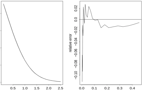
t(a) for a sequence of values of a, for the tilted bootstrap for this sample. Then we obtain 30000 tilted bootstrap samples from the original sample and get approximate tail area probabilities from these. These tail areas are plotted in the first panel of Figure 1 together with the saddlepoint approximation from Section 4 (We note that derivatives used in the saddlepoint approximation are calculated numerically without loss of accuracy). In the second panel we plot the relative errors. It is clear that throughout the range an excellent approximation is obtained, illustrating the results of Theorem 1.
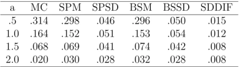
Table 1: Values a, Monte Carlo approximation, mean and standard deviation of 10 sad-dlepoint approximations to tilted bootstrap, mean and standard deviation of 10 tilted bootstrap approximations using 1000 bootstrap samples and standard deviation of the difference of the approximations.
a MC SPM SPSD BSM BSSD SDDIF .5 .314 .298 .046 .296 .050 .015 1.0 .164 .152 .051 .153 .054 .012 1.5 .068 .069 .041 .074 .042 .008 2.0 .020 .030 .028 .032 .028 .008
******************** Figure 1 about here ********************
We also consider the accuracy of the tilted bootstrap to the true distribution. We take 10000 Monte Carlo samples and for each sample compute ˆθ, S, and (ˆθ3 −θ30)/S.
We approximate the tail areas corresponding to ps(a) of the Studentised statistic for
a= (.5,1.0,1.5,2.0) using these 10000 Monte Carlo samples. Then we obtain 10 samples and from each we get 1000 tilted bootstrap samples from which we get approximate tail probabilities corresponding to the four values of a. The mean (BSM) and standard deviation (BSD) of these are given in Table 1. In addition, Table 1 gives the mean (SPM) and standard deviation (SPSD) of the 10 saddlepoint approximations corresponding to each of the four values of a. It also gives the standard error of the difference between the 10 pairs for eacha value (SDDIF). The tilted bootstrap and the saddlepoint are seen to be very close from the last column (SDDIF) and much of the small variation can be explained by the fact that only 1000 bootstrap samples were used. The approximation to the true distribution is not as good, as is to be expected from Theorems 3 and 4.
In addition, to examine the Studentised bootstrap, we took 3000 Monte Carlo samples and obtained approximations to the quantiles of (ˆθ3−θ30)/S, corresponding to frequencies
.2, .1, .05, .01. For each of the 3000 Monte Carlo samples we generate 100 nonparametric bootstrap samples, (Y∗
i , x∗i1, x∗i2) for i = 1,· · ·, n and for each of these we compute (θ∗3−
ˆ
the frequencies (out of 100) p∗ s(a) = P³ (θ∗ 3 −θˆ3)/S∗ ≥a ´
. This provides 3000 values for
p∗
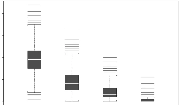
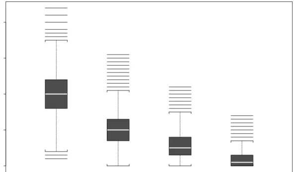
s(a) which are represented in the boxplots of Figure 2 and can be used to compare p∗s(a) with the exact tail areas .2, .1, .05, .01. These give boxplots as expected for 3000 random binomial (100, p) variates with p taking the values .2, .1, .05, .01. This is repeated with the tilted bootstrap to give Figure 3.
*********************** Figures 2 and 3 about here ***********************
Figures 2 and 3 show that the studentized bootstrap and the tilted bootstrap (which is not studentized) tail areas are equivalent. Both are centered around the exact values with the tilted bootstrap slightly less variable than the studentized bootstrap at least for the 0.2 and 0.1 tail areas.
6
Appendix
6.1
Conditions
Consider independent, identically distributed observations X1, X2,· · ·, Xn from a distri-bution F0. We have a score function ψ(X1, θ) which assumes values in ℜp such that
R
ψ(x, θ)dF0(x) = 0 has a solution θ0. Suppose that ψ(X1, θ) has a derivative ψ′(X1, θ)
with respect to θ, with probability 1, and assume (A1) det (R
ψ′(x, θ
0)dF0(x))6= 0.
Then, if for some γ > 0, R
ψ′(x, θ)dF
0(x) is continuous at all θ ∈ Bγp(θ0), the solution θ0
is the unique solution in Bp
γ(θ0), where by Bγp(θ0) we mean a cube with side length 2γ of
dimension p centered at θ0.
Assume that
(A2) The elements of ψ(X1, θ) and its first 4 derivatives with respect to θ exist and are
In order to apply an Edgeworth expansion we need a smoothness condition for the variables Uτ. Assume
(A3) 0 < c < detΣ1/2
τ < C and if ϕτ(ξ) = Eeiξ
TUτ
, then |ϕτ(ξ)| < 1−ρ, for ρ > 0 and for all c <|ξ|< Cnd/2, whered=p+q+r+ 1.
Choose 0< ǫ < 14|detE0ψ′(X1, θ0)|,γ >0 and B >0 and define the set E by
E =E(ǫ, γ, B) ={|det ¯Mθ−1Q¯θM¯θ−1|> ǫ, max|M¯θ′′|< B, |Lˆθ|< 3 4γ, for θ ∈B p γ(θ0)}. (6.17) Then the conditions (A1)-(A3) together with Cram´er’s large deviation theorem ensure that
P0(E)>1−e−cn
for some c >0 depending only on ǫ, γ, B. We can then restrict attention to X ∈E since for any event A
P0(A) =P0(A∩E) +O(e−cn)
and we will be concerned only with approximations to probabilities of events with errors at least O(e−cn). In the sequel we will restrict attention to samples in E. Then
||M¯θ−1( ¯Mθ0 −M¯θ)||< Bγ/ǫ <
1 4 for θ ∈ Bp
γ(θ0) by choice of γ < ǫ/4B. The inequality allows the application of Lemma
1 of Almudevar, Field and Robinson (2000) with α= 1/4 to show that there is a unique solutionT of Pn
j=1ψ(Xj, θ) = 0 in Bγp(θ0).
6.2
Proof of Theorem 2
Since in the problem considered here no densities exist we find the probability of the tail event {(T1 − θ10)/S ≥ y} by partitioning the space of (T, VT) into small regions and approximating P0((T1 −θ10)/S ≥ y) by summing probabilities of the appropriate
the space of (T, VT) by probabilities of regions in the space of ¯Uθ. These bounds are derived in the technical lemma below. Next we use indirect Edgeworth approximations to these probabilities and an integral approximation to the sum of the indirect Edgeworth approximations. As part of this we find bounds for the errors of approximation.
Lemma 1 Take θ ∈Bp3 4γ
(θ0), v ∈Rq and 0< δ < 14γ. Then there is a C > 0, depending
only on B, ǫ such that forδ chosen so that Cδ < 1
4, {Lˆθ ∈Bpδ(1−Cδ)(0)} ∩ {V¯θ+ ˆLθ[ ∂V¯θ ∂θ ]∈B q δ(1−Cδ)(v)}) ⊂ {T ∈Bδp(θ)} ∩ {V¯T ∈Bδq(v)} ⊂ {Lˆθ ∈Bδp(1+Cδ)(0)} ∩ {V¯θ+ ˆLθ[ ∂V¯θ ∂θ ]∈B q δ(1+Cδ)(v)}). (6.18)
Proof. Suppose T ∈Bδp(θ) and VT ∈Bδq(v). Expanding ¯LT = 0 about θ and noting that
inE,|M¯′
θ| are bounded and that |detM¯θ|> ǫ, we can choose
|Lˆθ−(θ−T)| ≤Cδ2 and then similarly
||V¯T −Vθ−Lˆθ[
∂V¯θ
∂θ ]|| ≤Cδ
2,
verifying the second inclusion of (6.18). Conversely, we can choose C such that sup θ′∈Bp δ(θ) |M¯θ−′1M¯θ−Ip| ≤ 1 2Cδ.
So from Lemma 1 of Almudevar, Field and Robinson (2000), if ˆLθ ∈ Bδp(1−Cδ)(0) and δ is such that Cδ < 1/4, then there is a unique solution T ∈ Bδp(θ). Also as before, if
¯ Vθ+ ˆLθ[∂ ¯ Vθ ∂θ ]∈B q δ(1−Cδ)(v), then ¯VT ∈B q
δ(v). This concludes the proof of the Lemma. We want P0((T1−θ10)/S ≥y) = P0({(T,V¯T)∈Bp3+q 4γ (θ0, E0V¯θ0)} ∩ {(T1−θ10)/S ≥y}) +O(e −cn). (6.19) Let (ζi, ηj, vk), where i, j, k take values · · ·,−2,−1,0,1,2,· · ·, be centers of cubes of side 2δ giving a partition of Rp+q with (ζ
0, η0, v0) = (θ10, θ20, E0V¯θ0). Denote by
P†
over {(i, j, k) : (ζi, ηj, vk) ∈ Bp3+q 4γ (θ0, E0V¯θ0) and ζi/s(ζi, ηj, vk) ≥ y}, where s(ζ, η, v) corresponds to S. Then P0((T1−θ10)/S ≥y) = X† P0((T1, T2,V¯T)∈Bδp+q(ζi, ηj, vk))(1 +O(δ)) +O(e−cn) (6.20) where the relative error O(δ) is due to using the cubes touching the boundary of the region {(T1−θ10)/S ≥y} withinBp3+q
4γ
(θ0, E0V¯θ0).
Now the lemma applied to the probability of this cube gives
P0({Lˆ(ζi,ηj) ∈B p δ(1−Cδ)(0)} ∩ {V¯(ζi,ηj)+ ˆL(ζi,ηj)[ ∂V¯θ ∂θ ]θ=(ζi,ηj) ∈B q δ(1−Cδ)(vk)}) < P0((T1, T2,V¯T)∈Bδp+q(ζi, ηj, vk)) < P0({Lˆ(ζi,ηj)∈B p δ(1+Cδ)(0)} ∩ {V¯(ζi,ηj)+ ˆL(ζi,ηj)[ ∂V¯θ ∂θ ]θ=(ζi,ηj) ∈B q δ(1+Cδ)(vk)}) Take Bkm to be a typical Bpδ(1−Cδ)(0)×B q δ(1−Cδ)(vk)×Bδr(wm), or by a similar term with 1−Cδ replaced by 1 +Cδ, where m takes values · · ·,−2,−1,0,1,2· · ·. The wm are centers of cubes of radius δ giving a partition of Rr with w
0 =E0( ¯Wθ0). We can bound the sum in (6.20) by X†X‡ P0(Z(ζi,ηj) ∈Bkm) +O(e −cn) where P‡
is a sum over m such that |wm|< 34γ and where for the lower bound Bkm has 1−Cδ and 1 +Cδ for the upper bound.
Writing u= (ℓ, v, w), let ed(u, Fτ) = exp(−nu∗Tu∗/2) (2π/n)(p+q+r)/2det Σ1/2 τ (1 + d X l=1 Qln(u∗√n)). Then using Theorem 1 of Robinson et al(1990), we have
P0(Zθ ∈Bkm) = P0(( ¯Lθ,V¯θ,W¯θ)∈g1−1(Bkm)) = enκ(τ(θ),θ)[ Z g−1 1 (Bkm) e−nℓTτ(θ)ed((ℓ, v, w), Fτ)dℓdvdw+R], (6.21) where R =R1+R2+R3 corresponding to the three residuals of Robinson et al (1990).
The first term in the last equation is equal to
enκ(τ(θ),θ) Z Bkm J1(z)e−nℓ Tτ(θ) ed(g1−1(z), Fτ)dz,
where J(z) is the Jacobian of the transformation z = g1(ℓ, v, w) and we write g1−1(z) =
(ℓ(z), v(z), w(z)). Noting that for this transformation g−11(0, v, w) = (0, v, w), we can approximate this integral by
P0(Zθ ∈B) = enκ(τ(θ),θ)[J1(0, vk, wm)ed((0, vk, wm), Fτ)δp+q+r(1 +O(nδ)) +R] Take δ = n−2 so that the term O(nδ) is O(n−1). Then noting that d = s−3 from
Theorem 1 of Robinsonet al(1990) and that our result concerns means rather than sums,
R1 < Cvol(g−11(B))n(p+q+r)/2−(d+1)/2 < Cvol(g1−1(B))n−1 (6.22)
if d=p+q+r+ 1, where vol(A) is the volume of the set A. Also
R3 < C sur(g−11(B))n(p+q+r)/2ǫ < Cvol(g1−1(B))n(p+q+r)/2ǫ/δ (6.23)
where ǫ is the smoothing parameter in the Theorem, where sur(A) is the surface area of the set A. Taking ǫ=n−(d+5)/2, we get
R3 < Cvol(g−11(B))n−1.
To bound the other term we use (A4) from which we see
R2 < Ce−cn. (6.24)
Approximating the sums by integrals, we have
P0((T1−θ10)/S≥y) = Z Ay enκ(τ(ζ,η),(ζ,η))J1(0, v, w)ed((0, v, w), Fτ)dζdηdvdw (1 +O(n−1)) + Z Ay enκ(τ(ζ,η),(ζ,η))dζdηdvdwO(n−1) (6.25) whereAy ={(ζ, η, v) :{(ζ−θ01)/s(ζ, η, v)≥y} ∩Bp3+q+r 4γ (θ10, θ20, E0V¯θ, E0W¯θ) and where we may incorporate the exponential error term in the relative error term by bounding y
Consider the transformation (ξ, η, v, w) =g2(ζ, η, v, w), where ξ = (ζ−θ10)/s(ζ, η, v)
with JacobianJ2(ξ, η, v, w). So we can write
P0((T1−θ10)/S ≥y) = Z ν y Z D e−nΛ(ξ,η,v,w)J 1J2 (2π/n)(p+q+r)/2detΣ1/2 τ dξdηdvdw(1 +O(1/n)) + + Z ν y Z De −nλ(ξ,η,v,w)dξdηdvdwO(n−1), (6.26)
where the first Edgeworth term in ed((0, v, w), Fτ) integrates to zero by symmetry and the other terms are in theO(1/n) relative error term, andνand the sides of the rectangle
D are chosen small enough so that (y, ν)×Dis in Bp3+q+r−1 4γ
(0, E0V¯θ0, E0W¯θ0), and so the
transformation is one to one and Λ(ξ, η, v, w) and λ(ξ, η, v, w) remain convex as functions of (ξ, η, v, w).
Now define H and h as in (2.5) and (2.6). Then using (A2)
P0((T1 −θ10)/S ≥y) = Z ν y e−nH(ξ) q 2π/nG(ξ)(1 +O(1/n)) +e −nh(ξ))O(1 n) dξ.(6.27) Putting w=w(ξ) =q2H(ξ) and w†(ξ) = w(ξ)−log(w(ξ)G(ξ)/H′(ξ))/nw(ξ) we can
obtain (2.7) of Theorem 2 as in Jing and Robinson (1994).
6.3
Proof of Theorem 3
In order to prove the result, we need to have an approximation for the tail area which is valid both under sampling from F0 and under bootstrap sampling. In particular the
approximation must be valid for the situation when the quantity of interest does not have a density. Theorem 2 gives such a result covering both cases since Condition (A3) still holds for the bootstrap (see Weber and Kokic (1998)). To apply Theorem 2 to the bootstrap, denote the cumulant generating function ofψ(X∗
1, θ) by
κ∗(τ, θ) = logX
exp(τTψ(xi, θ))/n. (6.28) Our interest is now in the approximation for the tail area
where P∗ denotes the probability computed under F
n and w†∗(a) is defined in the same way as w† in Theorem 2 with F
0 replaced by Fn.
Part of the argument follows closely that given in Section 2.1 of Feuerverger, Robinson and Wong (1999). To match their notation, write α(w(a)) = w(a)G(a)/H′(a) and note
that w†here corresponds to w∗ and α corresponds toψ in their paper. As bothw(a) and
α(w(a)) are analytic functions of y in a neighbourhood of the origin, we obtain
w(a) =A0+A1a+A2a2+A3a3+A4a4+O(a5)
and
α(w(a)) = B0+B1a+B2a2+B3a3+B4a4+O(a5),
where the coefficientsAj and Bj depend on the cumulants of ψ(Xi, θ) and its derivatives underFτ but not onn. We have a similar expression forw∗ andα∗(w∗) from the bootstrap
tail area.
By the same calculations as in the proof of Theorem 2 in Robinson, Ronchetti and Young (2003) we obtain
H(0) = 0, H′(0) = 0, H′′(0) = 1. (6.29) Therefore from the expansion ofw, we get A0 = 0 andA1 = 1. Moreover by equating the
integral in (6.27) taken over ℜ1 to 1, we obtain α(0) = 1 and thus B
0 = 1. We want to
consider the ratio
p∗ s(a) ps(a) = 1−Φ( √ nw†∗) 1−Φ(√nw†)[1 +O(1/n)] + e−nh(a)) 1−Φ(√nw†)O(1/n). (6.30)
The first term here is considered in the same way as in Section 2.1 of Feuerverger, Robinson and Wong (1999) and we can bound it by 1 +OP(√na3) for a < n−1/3. For the second term, we need to note that (6.29) holds and similarly thath(0) = 0, h′(0) = 0, h′′(0) = 1,
so −nh(a)/(1−Ψ(√nw†)) =O(na3). So if we restrict attention to a=O(n−1/3) we can
6.4
Proof of Theorem 4
In the case of the tilted bootstrap the cumulant generating function of ˜Fn is given by ˜ κ∗(τ, θ) = log(X ˜ wieτ Tψ(x i,θ)). (6.31)
This is used in Theorem 1 to obtain the saddlepoint approximation to the tilted bootstrap. We first prove the second order accuracy of the Edgeworth in this case. This is needed to obtain the comparisons of the expansions ofw†1(a) of Theorem 1 andw†(a) of Theorem
2, used later in the proof. The first part of the following proof is related to that of DiCiccio and Romano (1990) but differs in significant ways. We could use the general results of Hall (1992) to give the Edgeworth results but it is more transparent to write them out directly. For simplicity we will neglect all terms of smaller order thann−1/2 in the rest of
this section. We have
ps∗(a) = P∗((T1∗−t1)/S∗ ≥a) = P∗ à T∗ 1 −t1 s − S∗2−s2 2s3 a≥a ! = 1−Φ Ã √ na(1− acov(T ∗ 1, S∗2) s3 ! +√1 np( √ na)φ(√na) = 1−Φ(√na) + φ( √ na) √n à p(√na)−√na2cov(T ∗ 1, S∗2) s3 ! (6.32) and, if ˜s is the variance of T1 under the tilted distribution,
p∗t(a) = P˜∗(( ˜T1∗−θ10)/s≤a) = P∗(( ˜T∗ 1 −θ10)/s˜≤a(1−(˜s2−s2)/2s2)) = 1−Φ(√na(1−(˜s2−s2)/2s2)) + √1 np( √ na)φ(√na) = 1−Φ(√na) + φ( √na) √ n à p(√na)−√nas˜ 2−s2 2s2 ! . (6.33) To show that p∗ s(a)−p∗t(a) =o(1/ √ n)
we need to show ˜ s2 −s2 s2 =a cov(T∗ 1, S∗2) s3 . (6.34)
We can see that t−θ0 =BθT0L¯θ0, whereB
T θ0 = ¯M −1 θ0 and T ∗−t=BT t L¯t, so T1∗−t1 = BT
t1L¯t. Let ¯Yθ be the vector of all elements of ¯Mθ and ¯Qθ and letg( ¯Yθ) =s2 =BtT1QtBt1.
Then S∗2 =g( ¯YT∗) = g( ¯Yt) + ( ¯Yt∗−Y¯t)g′( ¯Yt) + (T∗−t) ∂Y¯t ∂t g ′( ¯Y t). So cov(T1∗, S∗2) =BtT1C12g′( ¯Yt) +BtT1C1Bt ∂Y¯t ∂t g ′( ¯Y t), where C12 = cov( ¯L∗t,Y¯t∗) andC1 = var( ¯L∗t).
Also ˜T∗
1 −θ10 = ˜BtT1
Pn
i=1ψ( ˜Xi∗,θ˜)/n and s2 = g( ¯Yt) and ˜s2 = g( ˜Yθ˜), where by ˜Yθ˜ we
mean weighted means of ψ(xi,θ˜) and similar terms with weights ˜wi. Then ˜ s2 =s2+ ( ¯Yθ˜−Y¯t)g′( ¯Yt) + ( ˜Yθ˜−Y¯θ˜)g′( ¯Yt).) (6.35) Now ¯Yθ˜−Y¯t = (˜θ−t)∂Y¯t/∂t and ˜ Yθ˜= n X i=1 ˜ wiYiθ˜= ¯Yθ0 +λB T t1C12
since ˜wi = 1/n+ ˜λBtT1ψ(xi, t). Also ˜λ = −(t−θ10)/s2 = −a/s and expanding in (4.11)
we have 1 n n X i=1 ψ(xi,θ˜) + ˜λ n X i=1 ψ(xi, t)ψ(xi, t)T = 0. Now ˜θ−t= ˜λBT
t Qt, so using these in (6.35) gives (6.34).
In order to obtain a result on the relative error, we can use Theorems 1 and 2 to get
p∗ s(a) p∗ t(a) = 1−Φ( √ nw∗ s) 1−Φ(√nw∗ t) (6.36) and then use Mill’s ratio to get
1−Φ(√nw∗
s) 1−Φ(√nw∗
t) ≤
We now expand the functionsw∗
s andw∗t. Since the expansion has the same form for each, we write an expansion for w∗ noting that the coefficients will differ for the two functions.
Now w∗(a) = a+A2a2+A3a3+. . .− log(1 +B1a+B2a2+. . .) n(a+A2a2+A3a3+. . .) = a+A2a2+A3a3+. . .−B1/n−aB2′/n+. . . As a result nw∗s(w∗s−w∗t) = na(A2s−A2t)a2+na(A3s−A3t)a3 −na(B1s−B1t)/n+. . .(6.38) Now A2s −A2t and B1s −B1t are both of order O(1/√n) from the equivalence of the Edgeworth expansions up to orderO(1/n) butA3s−A3t can only be shown to be of order
O(1). As a result we have that
1−Φ(√nw∗ s) 1−Φ(√nw∗ t) = 1 +O(na4∨n−1) (6.39) if we restrict a toO(n−1/3). Acknowledgements
The authors thank Joanna Flemming for her help with the computation of the numer-ical example.
References
Almudevar, A., Field, C. and Robinson, J. (2000). Saddlepoint density approximations for M-estimates. Ann. Statist., 28, 275-297.
DiCiccio, T. and Romano, J. (1990). Nonparametric confidence limits by resampling methods and least favorable families. Int. Statist. Rev.,58, 59-76
Feuerverger, A., Robinson, J. and Wong, A. (1999). On the relative accuracy of certain bootstrap procedures. Canad. J. Statist., 27, 225-236
Hall, P. (1992). The bootstrap and Edgeworth expansion, Springer, New York.
Jing, B.Y., Feuerverger, A. and Robinson, J. (1994). On the bootstrap saddlepoint ap-proximations. Biometrika., 81, 211-215.
Jing, B.Y., Kolassa, J. and Robinson, J. (2002). Partial saddlepoint approximations for transformed means. Scand. J. Statist., 29, 721-731.
Jing, B.Y., and Robinson, J. (1994). Saddlepoint approximations for marginal and con-ditional probabilities of transformed variables, Ann. Statist. 22, 1115-1132.
Robinson, J., H¨oglund, T., Holst, L. and Quine, M.P. (1990). On approximating proba-bilities for large and small deviations inRd. Ann. Prob.,18, 727-753.
Robinson, J., Ronchetti, E., Young, G.A. (2003). Saddlepoint approximations and tests based on multivariate M−estimates. Ann. Statist. 31, 1154-1169.
Robinson, J.and Skovgaard, I.M. (1998). Bounds for probabilities of small errors for empirical saddlepoint and bootstrap approximations. Ann. Statist. , 2369-2394.
Weber, N. and Kokic, P. (1997). On Cramer’s condition for Edgeworth expansions in the finite population case, Theory of Stochastic Processes, 3 (1997), 468-474.
C. FIELD
DEPARTMENT OF MATHEMATICS AND STATISTICS, DALHOUSIE UNIVERSITY,
HALIFAX, N. S., CANADA, B3H 3J5
E-Mail: [email protected]
J. ROBINSON
SCHOOL OF MATHEMATICS AND STATISTICS, UNIVERSITY OF SYDNEY, N.S.W. 2006, AUSTRALIA. E-Mail: [email protected] E. RONCHETTI DEPARTMENT OF ECONOMETRICS, UNIVERSITY OF GENEVA, GENEVA, SWITZERLAND E-Mail: [email protected]
Figure 1: The first panel gives tail probabilities for the saddlepoint approximation to the tilted bootstrap and approximate tail probabilities from 30000 tilted bootstrap samples
from one original sample. The second panel gives the relative errorss of these two approximations. u tt 0.5 1.0 1.5 2.0 2.5 0.0 0.1 0.2 0.3 0.4 tt relative error 0.0 0.1 0.2 0.3 0.4 −0.10 −0.08 −0.06 −0.04 −0.02 0.0 0.02
Figure 2: Boxplots of 3000 Studentised bootstrap p-values corresponding to exact tail areas 0.2, 0.1, 0.05,0.01. 0.0 0.1 0.2 0.3 0.4 .20 .10 .05 .01
Figure 3: Boxplots of 3000 tilted bootstrap p-values corresponding to exact tail areas 0.2, 0.1, 0.05,0.01. 0.0 0.1 0.2 0.3 0.4 .20 .10 .05 .01