Volume 5 | Number 1
Article 1
February 2018
Validating Geospatial Regression Models With
Bootstrapping
Lam T. Tran
Department of Biology, University of Pennsylvania, [email protected]
Phoebe Tran
Department of Chronic Disease Epidemiology, Yale School of Public Health, Yale University, [email protected]
Follow this and additional works at:
https://dc.uwm.edu/ijger
Part of the
Earth Sciences Commons
,
Environmental Sciences Commons
, and the
Geography
Commons
This Research Article is brought to you for free and open access by UWM Digital Commons. It has been accepted for inclusion in International Journal of Geospatial and Environmental Research by an authorized administrator of UWM Digital Commons. For more information, please contact [email protected].
Recommended Citation
Tran, Lam T. and Tran, Phoebe (2018) "Validating Geospatial Regression Models With Bootstrapping,"International Journal of Geospatial and Environmental Research: Vol. 5 : No. 1 , Article 1.
Spatial statistical models have been used extensively in many geospatial and environmental studies over several decades. While being very important, the issues of testing and validation in spatial statistical models are rarely investigated carefully in spatial environmental studies. Often strict theoretical asymptotic
assumptions used in those models are left unexplored or unanswered in many studies. This study is to explore if bootstrapping is capable of providing more realistic statistical inference for spatial regression models while dealing with several common issues with spatial data, such as spatial dependence and unknown
heteroscedasticity. With experiments on both simulated and real-world datasets, the study showed that bootstrapping can reveal the differences between empirical (bootstrap) distributions and those based on theoretical asymptotic assumptions in a forthright and sound fashion, allowing a spatial regression model to be validated effectively. Such validation arguably is very important to geospatial and environmental studies, especially those with small sample sizes. Hence, bootstrapping should be used widely as a second line of evidence for statistical inference in spatial environmental studies.
Keywords
spatial statistics, bootstrapping, statistical testing and validation, spatial lag/error regression Acknowledgements
The authors would like to acknowledge the guidance and support of Professor Warren Ewens, Department of Biology, University of Pennsylvania.
1. INTRODUCTION
Since its introduction in the field of spatial econometrics in the early 1980’s (Anselin 1988; Anselin and Bera 1998), spatial statistical analysis has found its way into many geospatial and environmental studies. Despite this long period of usage, whether spatial statistical model outputs, such as regression coefficients, which require various theoretical asymptotic assumptions, truly represent reality has often been left unexplored or unanswered in many studies. Inherited from conventional statistics, the asymptotic or large theory of test statistics for spatial model specification has been the subject of many studies (e.g., Cliff and Ord 1973; Sen,1976; King 1981; Anselin and Rey 1991; Anselin and Florax 1995; Anselin et al. 1996; Anselin and Kelejian,1997; Kelejian and Prucha 1999; Pinkse 2004). However, many spatial statistical analyses have small samples, which arguably do not satisfy those theoretical asymptotic requirements. One empirical approach to achieve robust estimation and testing in spatial statistical models is to utilize bootstrapping, which relies on resampling from observed data to approximate the probability distribution of the test statistics. Initially introduced by Efron (1979, 1982) for independent data, bootstrapping has been extended to deal with dependent data, especially time series data, by several authors (MacKinnon 2002; Davison et al. 2003; Horowitz 2003). For bootstrapping with spatially dependent data, earlier theoretical work has been done by Cliff and Ord (1973), Cressie (1980), and more recently Kelejian (2008). In general, bootstrapping has been proven to be a sound and effective alternative parameter estimate in cases where samples are finite and/or distributional assumptions for error terms cannot be verified. In environmental research, bootstrapping has been used to handle measurement errors in a number of studies (e.g., Madsen et al. 2008; Roberts and Martin 2008: Lopiano et al. 2011; Szpiro et al. 2011; Bergen et al. 2013; Szpiro and Paciorek 2013). However, the use of bootstrapping to explore the conformity between theoretical asymptotic assumptions in spatial statistical analyses and reality has rarely been seen in geospatial and environmental studies literature, at least from our review.
In this context, we explore in this paper the usefulness of bootstrapping in statistical testing and estimation in geospatial and environmental studies by applying the bootstrap to a spatial linear regression model on simulated datasets and a spatial dataset, which has been used in a number of studies. Our purpose is to illustrate that, by comparing the empirical bootstrap distributions of the estimates in spatial regression with those under theoretical asymptotic assumptions, an analyst would gain more confidence in the statistical inferences from the model and/or have more insights on potential issues that might influence the model’s results (spatial heteroscedasticity, heterogeneity in spatial relationship, etc.). The next section of data and methodology explains the dataset, spatial lag and error models, and the bootstrap methods. We then discuss the results from bootstrap simulations in the discussion section.
2. METHODS 2.1 Data
We utilized two simulated datasets and a real-world dataset, which has been used in a number of prior studies.
2.1.1. Simulated Dataset
We developed in this study two simulation scenarios (the two simulated datasets). For scenario 1, we first created a spatially-autocorrelated variable x1 on a regular 22x22
lattice in the form of:
x1= *W*x1 + (1)
where is a spatial autoregression parameter (specifically, =0.2128; see Appendix for detail), W is a spatial weight matrix (specifically, rook contiguity weights), and is a vector of a iid normal random variable (specifically, N(0, 1)). Next we created another variable, x2, which was correlated to x1 at a predefined level (e.g., the Pearson correlation
coefficient between x1 and x2 in scenario 1 was set at 0.9). For scenario 2, we used the
same simulated dataset of scenario 1 then created an outlier by changing one single point (x1, x2) in the dataset (e.g., from (0.6196, 0.1906) to (-7.0000, 0.1906)). Our intention
was to make the error term in the spatial lag and error regressions of x1 on x2 in scenario
2 no longer normally distributed. Figure 1 shows the layouts of x1 and x2 on 2222
lattices.
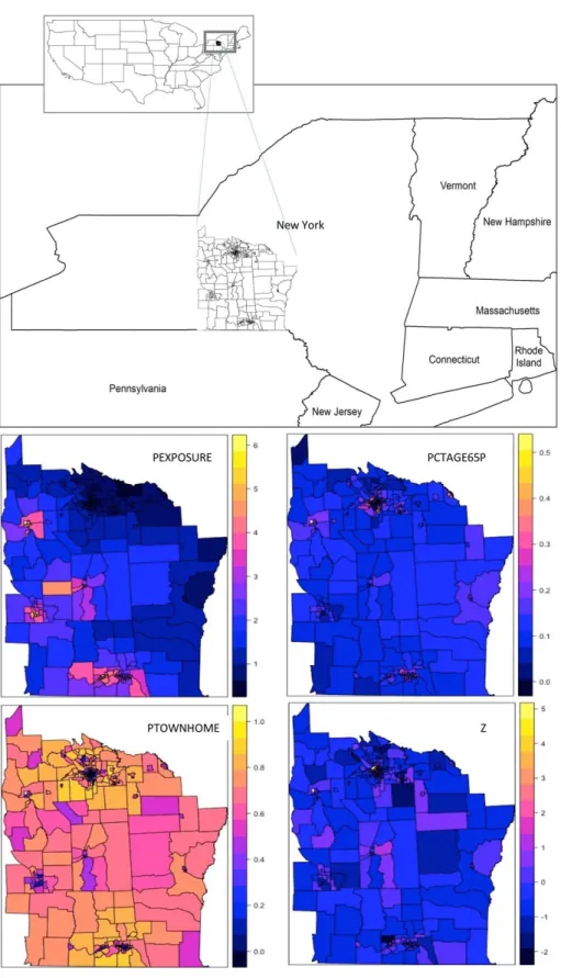
Figure 2. Map of the study area and layouts of the four variables in the New York Leukemia dataset used in the study.
2.1.2 Real-world Dataset
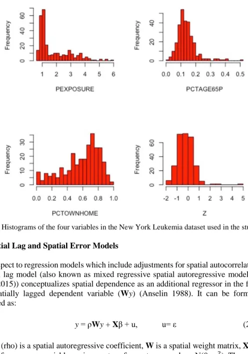
We utilized a dataset previously examined by Waller et al. (1992) to study the relationship between trichloroethylene (TCE, a suspected carcinogen) waste sites and leukemia in upstate New York between 1978 and 1982. The variables used in this analysis are listed in Table 1. Note that the dataset has been used in various epidemiological studies for different purposes (e.g., Waller and Turnbull 1993; Kulldorff and Nagarwalla 1995; Waller,1996; Gangnon and Clayton 1998; Ghosh et al. 1999; Rogerson 1999; Waller and Gotway 2004). Ahrens et al. (2001) augmented the dataset with demographic covariates from the 1980 census to shed more light on the relation between TCE waste sites and elevated leukemia rates. However, because we wanted to explore the usefulness of bootstrapping in a spatial study, we utilized a simple model with one dependent variable (Z, the transformed proportion of leukemia cases per tract) and three covariates (PCTOWNHOME, PCTAGE65P, and PEXPOSURE), essentially the same model presented in Waller and Gotway (2004). In other words, we did not intend to contribute to the understanding of the relationship between TCE and other covariates with leukemia rates. Figure 2 shows the study area and spatial layouts of these four variables. The histograms of the four variables as seen in Figure 3 were apparently skewed to differing extents and towards different directions. Accordingly, all four variables did not pass the Shapiro-Wilk normality test (p-values < 0.0001). Nevertheless, these four variables were used “as it is” (without any transformation) in the several linear regression analyses mentioned earlier. Utilizing this dataset in our analysis, we wanted to explore how untested and unsupported theoretical asymptotic assumptions in spatial regression analyses might influence a model’s results.
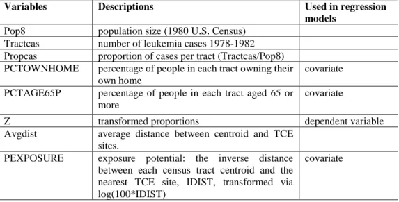
Table 1. Variables in the New York Leukemia dataset.
Variables Descriptions Used in regression
models
Pop8 population size (1980 U.S. Census)
Tractcas number of leukemia cases 1978-1982
Propcas proportion of cases per tract (Tractcas/Pop8)
PCTOWNHOME percentage of people in each tract owning their
own home
covariate PCTAGE65P percentage of people in each tract aged 65 or
more
covariate
Z transformed proportions dependent variable
Avgdist average distance between centroid and TCE
sites.
PEXPOSURE exposure potential: the inverse distance
between each census tract centroid and the nearest TCE site, IDIST, transformed via log(100*IDIST)
Figure 3. Histograms of the four variables in the New York Leukemia dataset used in the study.
2.2 Spatial Lag and Spatial Error Models
With respect to regression models which include adjustments for spatial autocorrelation, a spatial lagmodel (also known as mixed regressive spatial autoregressive model (de Smith, 2015)) conceptualizes spatial dependence as an additional regressor in the form of a spatially lagged dependent variable (Wy) (Anselin 1988). It can be formally expressed as:
y = ρWy + Xβ + u, u= ε (2) where ρ (rho) is a spatial autoregressive coefficient, W is a spatial weight matrix, X is a matrix of exogenous variables, u is a vector of error terms, and ε ~ N(0, 𝜎2). The usage of spatial lag model is considered proper when the focus is on determining the existence and strength of spatial interaction. Note that the spatial lag term Wy is correlated with the covariates even though they are independent and identically distributed (iid). This aspect can be seen from the reduced form of (2):
y = (I − ρW)-1Xβ + (I – ρW)-1 ε (3)
as well as the reduced form of the conditional expectation of y:
In contrast to the spatial lag model, a spatial error model places spatial dependence in the regression disturbance term (the nuisance dependence) (Anselin 1988). A spatial error model is formally expressed as:
y = Xβ + u, u=𝜆Wu + ε (5)
where 𝜆 (lambda) is the coefficient of the spatially-correlated errors. A spatial error model is appropriate when the focus is on dealing with the potentially bias-introducing influence of spatial autocorrelation due to the usage of spatial data. In this study, we applied both a spatial lag model and a spatial error model with the same set of covariates and dependent variable (see Table 1).
Regarding estimators, first outlined by Ord (1975), the maximum likelihood (ML) estimator is arguably the most common estimator used for spatial lag and error models (details on ML estimation in spatial lag and error models can be seen in Anselin 1988). The optimality properties of ML estimators (consistency, asymptotic efficiency, asymptotic normality) are established under a relatively strict classical framework, defined by Rao (1973). However, models with spatial dependence often do not fit such framework (Anselin, 2003). As a result, special attention needs to be given to the discrepancy between theoretical assumptions and real conditions, for example, on the restrictions on the variance and higher moments of the model variables, or the constraints on the range of dependence embraced in the spatial weight matrix (Kelejian and Prucha 1999; Anselin 2003) for more detail on these topics).
2.3 Bootstrap estimation in spatial regression models
Introduced by Efron (1979, 1982), bootstrapping is a robust estimator for alternative parameter estimates, measures of bias and variance, constructing confidence intervals (CIs), etc., by sampling with replacement from the original observations (e.g., Efron and Tibshirani 1993; Davison and Hinkley 1997; Chernick and LaBudde 2011). Bootstrapping has also been implemented in regression analyses (Freedman 1981; Bickel and Freedman 1982; Freedman and Peters 1984; Moulton and Zeger 1991). Bootstrapping in regression analysis can be carried out with two different approaches, one with residuals and the other with observation points. In the residual approach, the resampling is based on a set of regression residuals that is often obtained from a first-step estimation. Next, a bootstrap replication is constructed by randomly sampling with replacement from the first-step estimates to construct a pseudo dataset, and then combining it with the first-step estimates. Then, estimates of regression coefficients are derived by the same model and method as with the initial observed dataset in the first step. Repeating the process many times, the bootstrap estimates of regression coefficients create empirical distributions which in turn are used to derive different statistics (mean, CIs, etc.) for the regression coefficients. With the observation points approach, bootstrap replications are created by randomly sampling with replacement from the initial observed dataset, with empirical distributions of regression coefficients being formed in a similar fashion in the residual approach (see Freedman (1981), Freedman and Peters (1984), and Chernick and LaBudde (2011) for more details of bootstrapping in regression).
In spatial regression models, it is important to make sure that the random resampling retains the intrinsic spatial relationship of the dataset. In that context, Anselin
(1990) warned that a random sampling with just vectors [yi, (Wy)i, xi] for bootstrap
replication for a spatial lag model would not be sound (due to the endogeneity of the spatial lag term Wy). The same is true for a random sampling with bootstrapping just vectors [yi, xi] for a spatial error model because the intrinsic spatial relationship in the
error term (u=𝜆Wu + ε) might not be preserved properly. On the other hand, the residual approach is a sound alternative when the residuals from the first-step estimation can be randomly sampled to create pseudo error terms and consequently a pseudo-vector of dependent variables for both spatial lag and spatial error models as follows:
Initial model:
y = ρWy + Xβ + u (6)
Residuals e from first-step estimation of (6):
e = y – rWy – Xb (7)
and pseudo vector of dependent variable:
yr = (I − rW)-1Xb + (I – rW)-1 er* (8)
where r and b are consistent estimates for ρ and β, respectively, from first-step estimation; X are the fixed (exogenous) variables. Specifically, first-step estimates of r and b (rr and br) can be obtained by regressing yr on Wyr and (fixed) X. As the error
terms er (from first-step estimation) are assumed to be independent, the intrinsic spatial
relationship of the dataset is preserved. Because the normality assumption of the error term was not met, we used non-parametric bootstrapping instead (i.e., re-sampling the empirical distribution rather than from a specified model; see, for example, Davison and Hinkley (1997) and Chernick (2008), for more information on parametric and non-parametric bootstrap methods). Furthermore, to deal with heteroscedasticity in the error terms, we utilized the wild bootstrap method in which er* = er𝜈 with 𝜈 a random variable
with mean 0 and variance 1 (Wu 1986). There are different choices of 𝑣 mentioned in the literature (Liu 1988; Mammem 1993; Davidson and Flachaire 2008). We adopt the binary form of 𝜈 as follows:
𝜈𝑖 = { 1 𝑤𝑖𝑡ℎ 𝑝𝑟𝑜𝑏𝑎𝑏𝑖𝑙𝑖𝑡𝑦 1 2 −1 𝑤𝑖𝑡ℎ 𝑝𝑟𝑜𝑏𝑎𝑏𝑖𝑙𝑖𝑡𝑦 1 2 (9)
In term of estimator, we utilized the ML method for bootstrapping with the residual for both spatial lag and error models. In this study we ran bootstrap resampling 19,999 times for each model on the real-world dataset (9,999 times for the simulated datasets). For the sake of simplicity, without loss of generality, we used only two methods, the percentile method and the BCa method (bias-corrected bootstrap interval with the incorporation of an acceleration constant, to construct the 95% confidence intervals (CIs) for the regression coefficients of each model. While the bootstrap percentile method simply uses the distribution of bootstrap estimates to directly
construct the bootstrap confidence intervals, the BCa method makes correction for bias and skewness in the distribution of bootstrap estimates (Hall 1988). Details on these two bootstrap confidence interval methods as well as others (e.g., studentized, test-inversion, bias-corrected, etc.) can be found in various textbooks or review papers on bootstrap methods, such as DiCiccio and Efron (1996), Davison and Hinkley (1997), Carpenter and Bithell (2000), and Chernick (2008). Operationally, we ran first-step estimations of all regression models and their corresponding bootstrap analyses in R (R codes used in this study are available from the corresponding author on reasonable request). To measure the discrepancies between theoretical asymptotic distributions and those from empirical bootstrapping simulations, we calculated the overlap between confidence intervals from the initial models and those from bootstrap estimates as follows:
𝑜𝑣𝑒𝑟𝑙𝑎𝑝𝐶𝐼1−𝐶𝐼2=
min(𝑢𝑝𝑝𝑒𝑟 𝑏𝑜𝑢𝑛𝑑𝑠)−max (𝑙𝑜𝑤𝑒𝑟 𝑏𝑜𝑢𝑛𝑑𝑠)
max(𝑢𝑝𝑝𝑒𝑟 𝑏𝑜𝑢𝑛𝑑𝑠)−min (𝑙𝑜𝑤𝑒𝑟 𝑏𝑜𝑢𝑛𝑑𝑠) (10) We also calculated the overlap between bootstrap sampling distributions (i.e., histograms) and corresponding theoretical asymptotic distributions by a method described in Swain and Ballard (1991).
3. RESULTS & DISCUSSION 3.1 Simulated Datasets
Results of first-step estimates and their corresponding bootstrap estimates of the spatial lag and error model for scenarios 1 and 2 are shown in Table 2. Figure 4 shows the layouts of residuals of x1 regressed on x2, and residual histograms resulted from the initial
spatial lag and error models. In scenario 1, the error term in the spatial lag and spatial error regressions of x1 on x2 was iid and normally distributed (e.g., Shapiro-Wilk
normality test’s p-values = 0.9501 and 0.8468, respectively). Consequently, the bootstrapping results of both spatial lag and error models matched well with the corresponding estimates from the initial models. For example, the overlaps between bootstrap CIs and theoretical asymptotic CIs for all regression parameters were higher than 95% (except for the percentile CI of lambda in the spatial error model). A similar pattern was also observed between histograms of the bootstrap estimates and the corresponding scaled normal curves of initial models’ coefficient estimates (e.g., histogram overlaps > 94%). In scenario 2, with the presence of an outlier in the error term (Figure 3), such a high compatibility between initial models’ asymptotic estimates and bootstrap estimates were not really observed. The discrepancies were seen in both CIs and histograms between asymptotic and bootstrap estimates of rho and lambda, as well as in X2’s coefficient estimates for the spatial lag and spatial error models,
respectively (Table 2 and Figure 5). Hence, the bootstrap experiment on simulated datasets in this study shows that, compared to the initial models accompanied by various theoretical asymptotic assumptions which are often unsatisfied but untested/treated properly, bootstrapping can reveal more realistic inferential information for spatial regression models with small sample sizes and/or with other common spatial data issues (e.g., outlier in the error term).
Various studies have shown that theoretically and practically bootstrapping is able to handle various difficulties in regression modeling (e.g., unknown or non-Gaussian
error distribution, heteroscedasticity of variances, nonlinearity in the model parameters, and bias due to transformation) and provide a rational way to get the estimates of regression parameters (e.g., Freedman 1981; Duan 1983; Carroll and Ruppert 1988; Mammen 1993; Davison and Hinkley 1997; Chernick 2008; Chernick and LaBudde 2011). However, these strengths of bootstrapping in regression modeling have not been realized and/or applied widely in spatial regression modeling. In that context, the experiment in this study with two simulated datasets in two spatial (lag and error) regression models is only one example to illustrate the ability of bootstrapping in handling non-Gaussian error distribution in a spatial regression setting. On the other hand, bootstrapping has been observed to be inconsistent in some situations, such as distributions with infinite second moments (Davison and Hinkley 1997; Chernick 2008). While there are remedies for those situations (e.g., Chernick and LaBudde 2011), these topics have not been explored in detail in spatial regression modeling and certainly deserve more study in the future to fully understand the ability of bootstrapping (e.g., strengths/weaknesses, limitations) for different situations in spatial regression modeling. 3.2 Real-world Dataset
Table 3 displays results of first-step estimations (i.e., initial models) of the spatial lag and error models and their corresponding bootstrap estimates. Figure 6 shows histograms of bootstrap estimates of regression coefficients of the two models and the corresponding scaled normal curves of first-step model’s coefficient estimates. First of all, while the first-step estimations of the two models were different from one to another to some extent, those discrepancies are small and understandable due to the difference in the nature of the two models (spatial lag versus spatial error). Nevertheless, the results were very consistent between the spatial lag and error models in terms of which variables were statistically significant and what their significance levels were (e.g., PCTAGE65P significant at 0.0001-level and PCTOWNHOME at 0.05-level in the two models).
Overall, the empirical bootstrap CIs confirmed the statistical inference (significance/insignificance) of the estimations of PEXPOSURE, PCTAGE65P, and PCTOWNHOME, as well as those of lambda and rho, in the initial spatial lag and error models. However, CIs of the initial estimates, which are based on asymptotic assumptions, were different to empirical bootstrap CIs to different extents (e.g., varied from one variable to another and from one model to the other). The largest overlap between theoretical and empirical CIs in the spatial lag model belonged to PEXPOSURE followed by PCTOWNHOME and PCTAGE65P. On the other hand, PCTOWNHOME had the largest overlap between theoretical and empirical CIs in the spatial error model, followed by PEXPOSURE and PCTAGE65P. Note that PCTAGE65P had the smallest overlaps between theoretical and empirical CIs in both spatial lag and error models.
Figure 4. Layouts of residuals of x1 regressed on x2, and residual histograms resulted from the initial spatial lag and error models in scenarios 1 & 2
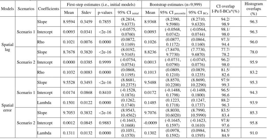
Table 2. First-step estimations (i.e., initial models) their corresponding bootstrap estimates on simulated datasets Models Scenarios Coefficients
First-step estimates (i.e., initial models) Bootstrap estimates (n=9,999) CI overlap
I-Pe/I-BCa*(%)
Histogram overlaps
(%) Mean Stdev p-values 95% CI initial Mean 95% CI percentile 95% CI BCa
Spatial lag Scenario 1 Slope 8.9594 0.3459 0.7855 (8.2814, 9.6373) 8.9368 (8.2390, 9.5980) (8.2710, 9.6320) 94.2/ 98.9 96.3 Intercept 0.0093 0.0341 <2e-16 (-0.0575, 0.0760) 0.0093 (-0.0568, 0.0742) (-0.0564, 0.0744) 98.1/ 98.0 96.3 Rho 0.1021 0.0076 0.0000 (0.0872, 0.1169) 0.1026 (0.0877, 0.1172) (0.0864, 0.1160) 97.3/ 94.4 96.0 Scenario 2 Slope 8.7678 0.3820 <2e-16 (8.0192, 9.5165) 8.8236 (7.8470, 9.7730) (7.7730, 9.6870) 77.7/ 78.2 78.0 Intercept 0.0000 0.0385 0.9999 (-0.0754, 0.0754) 0.0013 (-0.0731, 0.0790) (-0.0745, 0.0776) 96.2/ 98.0 95.9 Rho 0.1032 0.0083 0.0000 (0.0868, 0.1195) 0.1013 (0.0809, 0.1210) (0.0839, 0.1235) 81.5/ 82.6 83.2 Spatial error Scenario 1 Slope 9.5528 0.3493 <2e-16 (8.8681, 10.2375) 9.5488 (8.8570, 10.2200) (8.8690, 10.2290) 97.9/ 99.3 95.3 Intercept 0.0174 0.0868 0.8410 (-0.1528, 0.1876) 0.0172 (-0.1488, 0.1798) (-0.1488, 0.1800) 96.5/ 96.6 94.3 Lambda 0.1501 0.0122 0.0000 (0.1262, 0.1740) 0.1485 (0.1223, 0.1718) (0.1247, 0.1737) 88.2/ 96.3 93.9 Scenario 2 Slope 9.7053 0.3832 <2e-16 (8.9543, 10.4562) 9.7076 (8.8030, 10.6020) (8.7990, 10.5990) 83.5/ 83.4 85.3 Intercept 0.0012 0.0845 0.9883 (-0.1643, 0.1668) -0.0009 (-0.1645, 0.1597) (-0.1623, 0.1610) 97.8/ 97.6 95.8 Lambda 0.1311 0.0132 0.0000 (0.1051, 0.1570) 0.1302 (0.0978, 0.1592) (0.0984, 0.1595) 84.5/ 84.9 91.0
*% overlap between CIs, I-Pe: between initial model’s 95% CI and bootstrap percentile 95% CI; I-BCa: between initial model’s 95% CI and bootstrap BCa 95% CI.
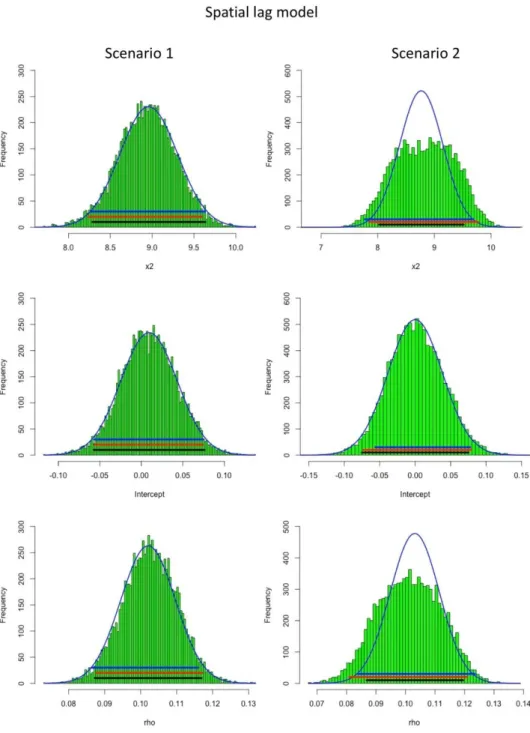
Figure 5. (a) Histograms of bootstrap estimates of spatial lag model’s coefficients and corresponding scaled normal curves of first-step model’s coefficient estimates, and CIs (black: initial model’s CIs, red or green: percentile CIs, blue: BCa CIs), in scenarios 1 & 2.
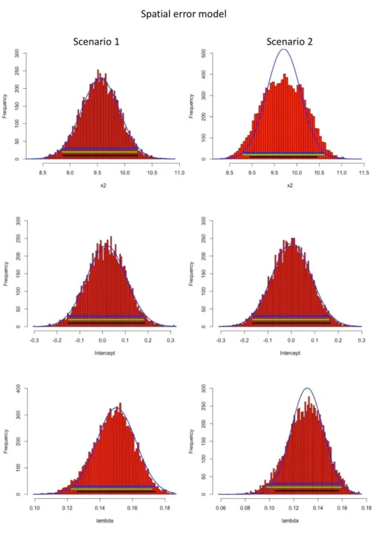
Figure 5. (b) Histograms of bootstrap estimates of spatial error model’s coefficients and corresponding scaled normal curves of first-step model’s coefficient estimates, and CIs (black: initial model’s CIs, red or green: percentile CIs, blue: BCa CIs), in scenarios 1 & 2.
Similar to the observations on CIs, there were discrepancies between the empirical bootstrap distributions of the regression coefficients and the corresponding scaled normal curves which were based on theoretical asymptotic assumptions. Comparing with their corresponding scaled normal curves, the empirical bootstrap distributions (of the coefficient) of PCTAGE65P were wider and flatter in both spatial
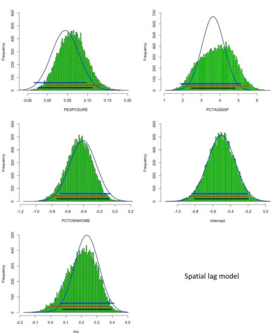
lag and error models. Furthermore, these empirical distributions of PCTAGE65P also failed the Shapiro-Wilk normality tests (e.g., p-values were <0.0001). For the spatial error model, while the empirical distributions of PEXPOSURE and PCTOWNHOME were different from their corresponding scaled normal curves, they still passed the Shapiro-Wilk normality tests (e.g., p-values were 0.9241 and 0.1469, respectively). For the spatial lag model, the empirical distribution of PEXPOSURE passed the Shapiro-Wilk normality tests value=0.1699), but those of PCTOWNHOME did not (p-value=0.0009). Note that discrepancies in CIs and distributions between empirical bootstrap results and those based on theoretical asymptotic assumptions (i.e., first-step estimates/initial models) were also observed in rho in the spatial lag model and in lambda of the spatial error model.
Arguably, with higher levels of conformity between empirical bootstrap simulations and the initial models’ estimates of PEXPOSURE and PCTOWNHOME, one would have more confidence in the statistical inferences for these two variables. In contrast, substantial discrepancies between bootstrap outcomes and the estimates of PCTAGE65P from the initial models would cause a researcher to be more cautious in using the initial models’ estimates of this variable. Note that there is a wide array of potential causes for discrepancies between empirical bootstrap results and estimates based on theoretical asymptotic assumptions, such as small sample size, spatial heteroscedasticity, spatial edge effect, heterogeneous spatial relationship, to name a few. While a bootstrap analysis like those in this study might not be able to identify a definite cause of those discrepancies, it can reveal the reality-versus-theory differences in a forthright and sound fashion, allowing a spatial regression model to be validated effectively. Such validation arguably is very important for geospatial and environmental studies, especially those with small sample sizes.
4. CONCLUSIONS
The purpose of the study was to show the ability of bootstrapping in revealing the difference between theory and reality, an important aspect but often ignored in spatial regression analyses. It is not uncommon that some theoretical assumptions used in spatial regression models are unsatisfied to some extent but the results of a regression model are still reasonable. However, proper test(s) should be carried out to validate the model. In that context, the bootstrap approach as illustrated in this paper is a suitable and sound tool for such purpose/test. This study also showed that bootstrapping can provide an alternative to empirically derive statistical inference for spatial regression models while effectively dealing with several common issues with spatial data, such as spatial dependence and unknown heteroscedasticity. Hence, bootstrapping should be used as a tool to validate estimates in spatial regression models. In other words, it can be a second line of evidence for statistical inference in geospatial and environmental studies, especially for those with small sample sizes.
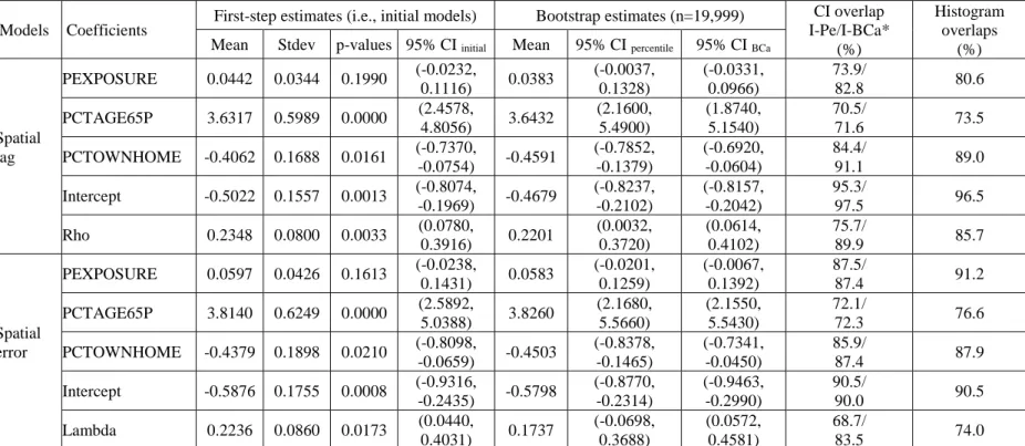
Table 3. First-step estimations of spatial lag and error models and their corresponding bootstrap estimates on the New York Leukemia dataset
Models Coefficients First-step estimates (i.e., initial models) Bootstrap estimates (n=19,999)
CI overlap I-Pe/I-BCa* (%) Histogram overlaps (%)
Mean Stdev p-values 95% CI initial Mean 95% CI percentile 95% CI BCa
Spatial lag PEXPOSURE 0.0442 0.0344 0.1990 (-0.0232, 0.1116) 0.0383 (-0.0037, 0.1328) (-0.0331, 0.0966) 73.9/ 82.8 80.6 PCTAGE65P 3.6317 0.5989 0.0000 (2.4578, 4.8056) 3.6432 (2.1600, 5.4900) (1.8740, 5.1540) 70.5/ 71.6 73.5 PCTOWNHOME -0.4062 0.1688 0.0161 (-0.7370, -0.0754) -0.4591 (-0.7852, -0.1379) (-0.6920, -0.0604) 84.4/ 91.1 89.0 Intercept -0.5022 0.1557 0.0013 (-0.8074, -0.1969) -0.4679 (-0.8237, -0.2102) (-0.8157, -0.2042) 95.3/ 97.5 96.5 Rho 0.2348 0.0800 0.0033 (0.0780, 0.3916) 0.2201 (0.0032, 0.3720) (0.0614, 0.4102) 75.7/ 89.9 85.7 Spatial error PEXPOSURE 0.0597 0.0426 0.1613 (-0.0238, 0.1431) 0.0583 (-0.0201, 0.1259) (-0.0067, 0.1392) 87.5/ 87.4 91.2 PCTAGE65P 3.8140 0.6249 0.0000 (2.5892, 5.0388) 3.8260 (2.1680, 5.5660) (2.1550, 5.5430) 72.1/ 72.3 76.6 PCTOWNHOME -0.4379 0.1898 0.0210 (-0.8098, -0.0659) -0.4503 (-0.8378, -0.1465) (-0.7341, -0.0450) 85.9/ 87.4 87.9 Intercept -0.5876 0.1755 0.0008 (-0.9316, -0.2435) -0.5798 (-0.8770, -0.2314) (-0.9463, -0.2990) 90.5/ 90.0 90.5 Lambda 0.2236 0.0860 0.0173 (0.0440, 0.4031) 0.1737 (-0.0698, 0.3688) (0.0572, 0.4581) 68.7/ 83.5 74.0
*% overlap between CIs, I-Pe: between initial model’s 95% CI and bootstrap percentile 95% CI; I-BCa: between initial model’s 95% CI and bootstrap BCa 95% CI.
Figure 6. (a) Histograms of bootstrap estimates of spatial lag model’s coefficients and corresponding scaled normal curves of first-step model’s coefficient estimates, and CIs (black: initial model’s CIs, red or green: percentile CIs, blue: BCa CIs), for the real-world dataset.
Figure 6. (b) Histograms of bootstrap estimates of spatial error model’s coefficients and corresponding scaled normal curves of first-step model’s coefficient estimates, and CIs (black: initial model’s CIs, red or green: percentile CIs, blue: BCa CIs), for the real-world dataset.
APPENDIX
x1 in the simulated datasets was created with the following R codes:
=0.2128 was resulted from a specific setting of μ (mu) at 40 and the random component with a normal distribution N(0,1).
REFERENCES
Ahrens, C., Altman, N., Casella, G., Eaton, M., Hwang, J.T.G., Staudenmayer, J. and Stefanescu, C. (2001) Leukemia clusters in upstate New York: how adding covariates changes the story. Environmetrics, 12, 659-672.
Anselin L. (2003) Spatial Econometrics. In B.H. Baltagi (Ed.). A Companion to Theoretical Econometrics (pp. 310-330). Wiley-Blackwell: Malden, MA. Anselin, L. (1988) Spatial Econometrics: Methods and Models. Kluwer: Dordrecht. Anselin, L. (1990) Some robust approaches to testing and estimation in spatial
econometrics. Regional Science and Urban Economics,20, 141-163.
Anselin, L., Bera, A.K., Florax, R. and Yoon, M. (1996) Simple diagnostic tests for spatial dependence. Regional Science and Urban Economics, 26, 77-104. Anselin, L. and Bera. A.K. (1998) Spatial dependence in linear regression models with
an introduction to spatial econometrics. In A. Ullah & D. Giles (Eds.).
Handbook of Applied Economic Statistics (pp. 237-289). New York: Marcel Dekker.
Anselin, L. and Florax, R. (1995) Small sample properties of tests for spatial dependence in regression models: some further results. In L. Anselin & R. Florax (Eds.). New Directions in Spatial Econometrics (pp. 21-74). Spinger Verlag: New York.
Anselin, L. and Kelejian, H. (1997) Testing for spatial autocorrelation in the presence of endogenous regressors. International Regional Science Review, 20, 1-2, 153–182.
Anselin, L. and Rey, S. (1991) Properties of tests for spatial dependence in linear regression models. Geographical Analysis, 23, 112-131.
# Create an empty matrix and spatial coordinates of its cells
side=22
fullSize<-side*side
my.mat <- matrix(NA, nrow=side, ncol=side) x.coord <- rep(1:side, each=side)
y.coord <- rep(1:side, times=side) xy <- data.frame(x.coord, y.coord)
# Create a random component across the 22x22 lattice
ZZZ<-rnorm(latticeSize, 0, 1)
# Use Principal Coordinates of Neighborhood Matrix (from 'vegan' package) to # create a spatial autocorrelation component.
pcnm.axes <- pcnm(xy.dist)$vectors
# Change mu to have different spatial autocorrelation degrees: large mu (e.g., >100) # for higher spatial correlation, and small mu (e.g., =10) for more random pattern
mu=40
# Create a spatial dataset with some spatial autocorrelation level and randomness
Bergen, S., Sheppard, L., Sampson, P.D., Kim, S.Y., Richards, M., Vedal, S., Kaufman, J.D. and Szpiro, A.A. (2013) A national prediction model for PM2.5 component exposures and measurement error-corrected health effect inference. Environmental Health Perspectives, 121, 9, 1017-1025.
Bickel, P. and Freedman, D.A. (1982) Bootstrap Regression Models with Many Parameters. Department of Statistics, University of California at Berkeley, Technical Report No.7: Berkeley, CA.
Carpenter, J. andBithell, J. (2000) Bootstrap confidence intervals: when, which, what?
A practical guide for medical statisticians. Stat Med., 19, 9, 1141-1164.
Carroll, R.J. and Ruppert, D. (1988) Transformations and Weighting in Regression.
Chapman & Hall: New York.
Chernick, M.R. (2008) Bootstrap Methods: A Guide for Practitioners and Researchers.
Wiley-Interscience: Hoboken, New Jersey (2nd ed.).
Chernick, M.R. and LaBudde, R.A. (2011) An Introduction to Bootstrap Methods with Applications to R. Wiley: Hoboken, New Jersey.
Cliff, A. and Ord, J. (1973) Spatial Autocorrelation. Pion: London. Cressie, N.A.C. (1980) Statistics for Spatial Data. Wiley: New York.
Davidson, R. and Flachaire, E. (2008) The wild bootstrap, tamed at last. Journal of
Econometrics, 146, 1, 162-169.
Davison, A.C. and Hinkley, D.V. (1997) Bootstrap Methods and their Application. Cambridge University Press: London.
Davison, A.C., Hinkley, D.V. and Young, G.A. (2003) Recent developments in bootstrap methodology. Statistical Science, 18, 141-157.
de Smith, M.J. (2015) STATSREF: Statistical Analysis Handbook - a web-based statistics resource. The Winchelsea Press, Winchelsea, UK
DiCiccio, T.J. and Efron, B. (1996) Bootstrap confidence intervals. Statistical Science, 11, 189–212.
Duan, N. (1983) Smearing estimate a nonparametric retransformation method. J. Am. Stat. Assoc., 78, 605–610.
Efron, B. (1979) Bootstrap methods, another look at the jackknife. Annals of Statistics, 7, 1-26.
Efron, B. (1982) The Jackknife, the Bootstrap and Other Resampling Plans. Society for Industrial and Applied Mathematics, Philadelphia, PA.
Efron, B. (1987) Better bootstrap confidence intervals (with discussion). J. Amer. Statist. Assoc., 82(397), 171-185.
Efron, B. and Tibshirani, R. (1993) An Introduction to the Bootstrap. Chapman & Hall: New York.
Freedman, D.A. (1981) Bootstrapping regression models. Annals of Statistics, 9, 1218-1228.
Freedman, D.A. and Peters, S.C. (1984) Bootstrapping a regression equation: Some empirical results. Journal of the American Statistical Association, 79, 385, 97-106.
Gangnon, R.E. and Clayton, M.K. (1998) Bayesian Spatial Disease Clustering: An Application. Technical Report #132. Department of Biostatistics, University of Wisconsin, Madison.
Ghosh, M., Natarajan, K., Waller, L. and Kim, D. (1999) Hierarchical Bayes GLMs for the analysis of spatial data: an application to disease mapping. Journal of Statistical Planning and Inference, 75, 2, 305-318.
Hall, P. (1988) Theoretical comparison of bootstrap confidence intervals (with discussion). Ann. Statist., 16, 927-985.
Horowitz, J.L. (2003) The bootstrap in econometrics. Statistical Science, 18, 211-218. Kelejian, H. (2008) A spatial J-test for model specification against a single or a set of
non-nested alternatives. Letters in Spatial and Resource Sciences, 1, 3-11. Kelejian, H. and Prucha, I.R. (1999) A generalized moments estimator for the
autoregressive parameter in a spatial model. International Economic Review, 40, 509–33.
King, M. (1981) A small sample property of the Cliff-Ord test for spatial correlation.
Journal of the Royal Statistical Society B, 43, 263-264.
Kulldorff, M. and Nagarwalla, N. (1995) Spatial disease clusters: detection and inference. Statist. Med., 14, 799–810
Liu, R.Y. (1988) Bootstrap procedure under some non-iid models. Annals of Statistics, 16, 1696-1708.
Lopiano, K.K., Young, L.J. and Gotway, C.A. (2011) A comparison of errors in variables methods for use in regression models with spatially misaligned data.
Statistical Methods in Medical Research,20, 1, 29–47.
MacKinnon, J.G. (2002) Bootstrap inference in econometrics. Canadian Journal of Economics, 35, 615–645.
Madsen, L., Ruppert, D. and Altman, N.S. (2008) Regression with spatially misaligned data. Environmetrics, 19, 453–467.
Mammen, E. (1993) Bootstrap and wild bootstrap for high dimensional linear models.
Annals of Statistics, 21, 255-285.
Moulton, L.H. and Zeger, S.L. (1991) Bootstrapping generalized linear models.
Computational Statistics & Data Analysis, 11, 53-63.
Ord, J.K. (1975) Estimation methods for models of spatial interaction. Journal of the American Statistical Association, 70, 120–6.
Pinkse, J. (2004) Moran-flavoured tests with nuisance parameters: Examples. In L. Anselin, R. Florax & S. Rey (Eds.). Advances in Spatial Econometrics (pp. 67-77). Springer- Verlag: Berlin.
Rao, C.R. (1973) Linear Statistical Inference and its Applications.Wiley:New York Wiley (2nd ed).
Roberts, S. and Martin, M.A. (2010) Bootstrap-after-bootstrap model averaging for reducing model uncertainty in model selection for air pollution mortality studies. Environmental Health Perspectives, 118, 1, 131-136. doi:10.1289/ehp.0901007.
Rogerson, P. (1999) The detection of clusters using a spatial version of the chi-square goodness-of-fit statistic. Geographical Analysis, 31, 1, 130-147.
Sen, A. (1976) Large sample size distribution of statistics used in testing for spatial correlation. Geographical Analysis, 8, 2, 175-184.
Swain, M. and Ballard, D. (1991) Color indexing. Intl. Journal of Computer Vision, 7, 1,11–32.
Szpiro, A.A. and Paciorek, C.J. (2013) Measurement error in two-stage analyses, with application to air pollution epidemiology. Environmetrics, 24, 501–17. Szpiro, A.A., Sheppard, L. and Lumley, T. (2011) Efficient measurement error
correction with spatially misaligned data. Biostatistics, 12, 4, 610–623. Waller, L. (1996) Statistical power and design of focused clustering studies. Statistics
Waller, L. and Gotway, C.A. (2004) Applied Spatial Statistics for Public Health Data. Wiley: Hoboken, New Jersey.
Waller, L. and Turnbull, B. (1993) The effects of scale on tests for disease clustering.
Statistics in Medicine, 12, 1869-1884.
Waller, L., Turnbull, B., Clark, L. and Nasca, P. (1992) Chronic disease surveillance and testing of clustering of disease and exposure: application to leukemia incidence in TCE-contaminated dumpsites in upstate New York.
Environmetrics, 3, 281-300.
Wu, C.F.J. (1986) Jackknife, bootstrap and other resampling methods in regression analysis. Annals of Statistics, 14, 1261-1295.