OpenBU http://open.bu.edu
Theses & Dissertations Boston University Theses & Dissertations
2017
Assessing malware detection using
hardware performance counters
https://hdl.handle.net/2144/27051 Boston University
COLLEGE OF ENGINEERING
Thesis
ASSESSING HARDWARE PERFORMANCE COUNTERS
FOR MALWARE DETECTION
by
ANMOL GUPTA
B.E., Mumbai University, 2015
Submitted in partial fulfillment of the
requirements for the degree of
Master of Science
First Reader
Manuel Egele, PhD
Assistant Professor of Electrical and Computer Engineering
Second Reader
Ajay Joshi, PhD
Associate Professor of Electrical and Computer Engineering
Third Reader
Michel Kinsy, PhD
First and foremost, I am endlessly thankful to my advisor, professor Manuel Egele and my co-advisor, professor Ajay Joshi – without whom this work would not have been possible. Their help and support, despite my constant resistance, was the only thing that brought me where I am right now. A special mention to the collaborators and contributors of this project. It goes without saying without the contributions of Boyou Zhou, this project would have never reached its summit. With him, I would also like to thank Leila Delshadtehrani who was always on her feet to help me out.
I would like to express gratitude to my parents, Brijesh and Shobha Gupta, as they were the ones who encouraged me to take on this path, and were morally very helpful throughout. My parents together with my young sibling brother, Devansh Gupta, were there when I needed them the most, and thus should always be thanked for believing in me.
Lastly, I would like to mention all my colleagues in the infamous PHO 340 and PHO 301 rooms, with whom I spent enormous amount of time having off-topic discussions on completely irrelevant topics - Yenai, Fulya, Saiful, Onur(x2), Ozan, QuingQuing, Rushi, Ahmed, Ethan, Zafar, Asselya, Kiran, Aravind, Furkhan and Sadullah. With the conclusion of this project began a new string of invaluable friend-ship.
Anmol Gupta Boston University ECE Department
FOR MALWARE DETECTION
ANMOL GUPTA
ABSTRACT
Despite the use of modern anti-virus (AV) software, malware is a prevailing threat to today’s computing systems. AV software cannot cope with the increasing num-ber of evasive malware, calling for more robust malware detection techniques. Out of the many proposed methods for malware detection, researchers have suggested microarchitecture-based mechanisms for detection of malicious software in a system. For example, Intel embeds a shadow stack in their modern architectures that main-tains the integrity between function calls and their returns by tracking the function’s return address. Any malicious program that exploits an application to overflow the return addresses can be restrained using the shadow stack. Researchers also propose the use of Hardware Performance Counters (HPCs). HPCs are counters embedded in modern computing architectures that count the occurrence of architectural events, such as cache hits, clock cycles, and integer instructions. Malware detectors that leverage HPCs create a profile of an application by reading the counter values pe-riodically. Subsequently, researchers use supervised machine learning-based (ML) classification techniques to differentiate malicious profiles amongst benign ones. It is important to note that HPCs count the occurrence of microarchitectural events during execution of the program. However, whether a program is malicious or benign is the high-level behavior of a program. Since HPCs do not surveil the high-level behavior of an application, we hypothesize that the counters may fail to capture the difference in the behavioral semantics of a malicious and benign software.
recreate the experimental setup from the previously proposed systems. To this end, we leverage HPCs to profile applications such as MS-Office and Chrome as benign applications and known malware binaries as malicious applications. Standard ML classifiers demand a normally distributed dataset, where the variance is independent of the mean of the data points. To transform the profile into more normal-like dis-tribution and to avoid over-fitting the machine learning models, we employ power transform on the profiles of the applications. Moreover, HPCs can monitor a broad range of hardware-based events. We use Principal Component Analysis (PCA) for se-lecting the top performance events that show maximum variation in the least number of features amongst all the applications profiled. Finally, we train twelve supervised machine learning classifiers such as Support Vector Machine (SVM) and MultiLayer Perceptron (MLPs) on the profiles from the applications. We model each classifier as a binary classifier, where the two classes are ‘Benignware’ and ‘Malware.’ Our results show that for the ‘Malware’ class, the average recall and F2-score across the twelve classifiers is 0.22 and 0.70 respectively. The low recall score shows that the ML classifiers tag malware as benignware. Even though we exercise a statistical approach for selecting our features, the classifiers are not able to distinguish between malware and benignware based on the hardware-based events monitored by the HPCs. The incapability of the profiles from HPCs in capturing the behavioral characteristic of an application force us to question the use of HPCs as malware detectors.
1 Introduction 1
1.1 Motivation . . . 1
1.2 Contributions . . . 4
1.3 Related Work . . . 6
1.4 Background . . . 9
1.4.1 Hardware Performance Counters . . . 9
1.4.2 Hardware Performance Events . . . 11
1.4.3 Malware and Malware Detection . . . 13
1.4.4 Principal Component Analysis . . . 15
1.4.5 Power Transform . . . 18
2 Malware Detector using HPCs 21 2.1 Profilers - Introduction . . . 21
2.2 Savitor . . . 25
2.3 Benignware and Malware Used . . . 29
2.4 Feature Extraction . . . 31
2.5 Feature Selection . . . 33
2.6 Machine Learning Classifiers . . . 36
3 Evaluation 37 3.1 Experimental Setup . . . 37
3.2 Results after Feature Selection using PCA . . . 42
3.3 Metrics to measure Classification Accuracies . . . 46 viii
3.5 Classification Results - Intel . . . 54
4 Conclusions 59
4.1 Summary of the thesis . . . 59 4.2 Future Work . . . 61
References 63
Curriculum Vitae 69
1.1 Classes of Malware [Demme et al., 2013], [Risks, 2011] . . . 14
2.1 Predefined Options to profile on AMD’s CodeAnalyst . . . 22
2.2 Events profiled for Access Performance Profiling on AMD’s CodeAnalyst 23 2.3 Events profiled for Time-based Profiling on AMD’s CodeAnalyst . . . 23
2.4 Task List of the threads in Savitor . . . 27
2.5 Django, Tornado and SQLite services used as benignware . . . 30
2.6 Supervised Machine Learning Classifiers . . . 36
3.1 Experimental Setup - Specifications . . . 41
3.2 List of Top 6 AMD Events Code & Description . . . 42
3.3 List of Top 4 Intel Events Code & Description . . . 42
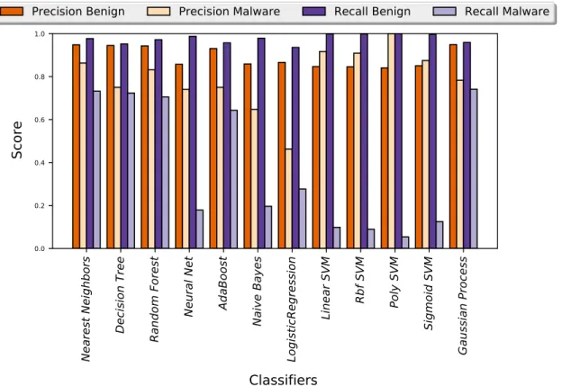
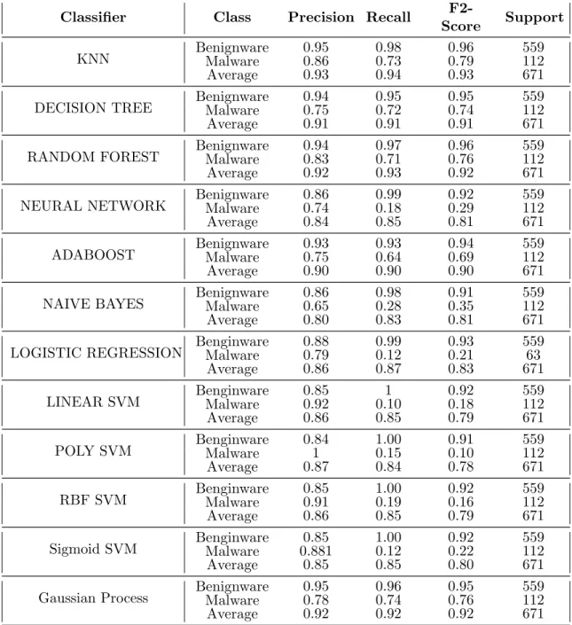
3.4 Classifier results in terms of Precision, Recall, F2-Score and Support for each class on the AMD machine. [F2-Score is weighted harmonic mean for each class, whereas the Average is weighted mean of Precision, Recall, and F2-Score values for benignware and the malware classes individually.] . . . 49
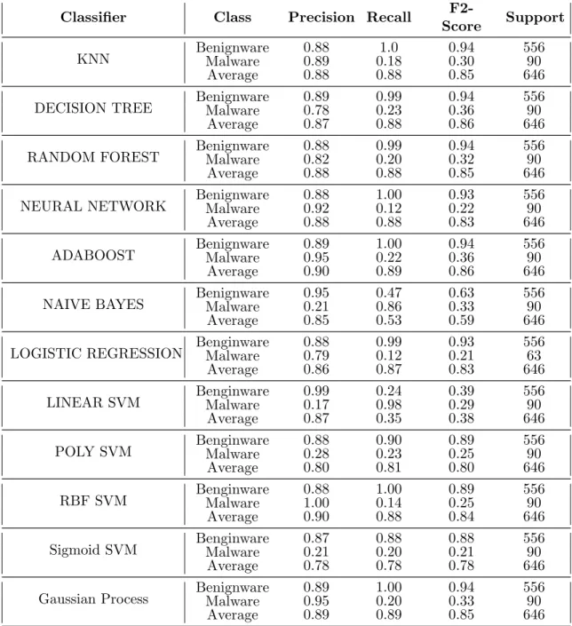
3.5 Classifier results in terms of Precision, Recall, F2-Score and Support for each class on the Intel machine . . . 55
1·1 Various architectural events available to monitor on the HPCs . . . . 12 1·2 PCA demonstration - Converting a 3-dimensional original data space
to a 2-dimensional linearly uncorrelated components [Vidhya, 2016] . 16 1·3 Logarithmic Function [Scibilia, 2015] . . . 20 2·1 Variation in dataset: (a) A non-normal distribution #1; and (b)
Nor-mal (Gaussian) Distribution #2. [University of Minnesota, 2017] . . 32 3·1 Executing and Profiling Malware using Savitor and Intel’s VTunes . . 39 3·2 Scree and Cumulative Variation Plot for Intel’s Top 4 events . . . 44 3·3 Scree and Cumulative Variation Plot for AMD’s Top 6 events . . . . 45 3·4 Precision and Recall Scores for classification of benignware and
Mal-ware Classes for the AMD experimental setup. . . 48 3·5 2D representation of the entire Data space, the training data space and
the testing data space. . . 51 3·6 a. ROC Curve for all the classifiers. b. ROC-Area Under Curve
(AUC) and Cross-validation score for all the classifiers . . . 53 3·7 Precision and Recall Scores for classification of benignware and
Mal-ware Classes for the Intel’s experimental setup. . . 54 3·8 2D representation of the entire Data space, the training data space and
the testing data space. . . 56 3·9 a. ROC Curve for all the classifiers. b. ROC-Area Under Curve
(AUC) and Cross-validation score for all the classifiers . . . 58 xi
AMD . . . Advanced Micro Devices
API . . . Application Programming Interface ARM . . . Advanced RISC Machines
AV . . . Anti-Virus
CWT . . . Continuous Wavelet Transform DT . . . Decision Trees
DWT . . . Discrete Wavelet Transform EBP . . . Event-based Profiling FN . . . False Negative
FP . . . False Positive
GUI . . . Graphical User Interface
HPC . . . Hardware Performance Counter ISA . . . Instruction Set Architecture KNN . . . K-Nearest Neighbor
ML . . . Machine Learning MPL . . . MultiLayer Perceptron MSR . . . Model Specific Registers NI . . . National Instruments OS . . . Operating System PC . . . Principal Component
PCA . . . Principal Component Analysis PMC . . . Performance Monitoring Counter PMU . . . Performance Monitoring Unit SD . . . Standard Deviation
SMI . . . System Management Interrupt SMM . . . System Management Mode SVM . . . Support Vector Machines TBP . . . Time-Based Profiling
TLB . . . Translation Lookaside Buffer TN . . . True Negative
TP . . . True Positive VM . . . Virtual Machine WT . . . Wavelet Transform
R2 . . . the Real plane
Chapter 1
Introduction
1.1
Motivation
Leveraging the low-level micro architectural features for providing security is a grow-ing trend among hardware companies. For example, Advanced RISC Machines (ARM) [ARM, 2017a] provides TrustZone [ARM, 2017b]. TrustZone architecturally divides the hardware into a secure and insecure zone running secure OS and normal OS re-spectively. The hardware-separated ‘secure’ and ‘insecure’ zones are used to separate the execution of user-level applications from the trusted kernel operations. Security is thus maintained using the existing hardware of the device, without affecting system performance. Qualcomm’s Snapdragon 835 Mobile Platform usesHaven [Qualcomm, 2017] which is a combination of hardware and biometric technologies to secure fi-nancial transactions over the Internet. Intel’s 4th generation Instruction Set Archi-tecture (ISA) has dedicated instructions, called AES-NI [Akdemir et al., 2010], for providing fast and secure encryption-decryption using Advanced Encryption Stan-dards (AES) [Rijmen and Daemen, 2001]. Additionally, Intel also provides platform security by securing the BIOS, the firmware and hardware-based authentication us-ing Boot Guard, BIOS Guard, and Identity Protection Technology (IPT) [Intel, 2017].
The hardware implementations of security features mentioned above provide energy-efficient, low-overhead, and high-performance solutions compared to their software counterparts. However, developing dedicated hardware support for security leads
to a substantially longer time-to-market than software products. National Instru-ments(NI) state that a hardware product takes on average a year or more to mature from the idea stage to production stage [Instruments, 2014]. Moreover, there is a per-sistent race between the security developers and their adversaries. One approach for keeping pace in this persistence race between the malware developers and security de-velopers is leveraging the existing hardware units to implement defense mechanisms. Recently, researchers have proposed to use Hardware Performance Counters (HPCs) for malware detection [Demme et al., 2013], [Bahador et al., 2014], [Patel et al., 2017]. HPCs are physical counters embedded in modern processors. These counters are ca-pable of counting the occurrence of a wide range of low-level architectural events such as branch mispredictions and data cache hits. Initially, software designers employed HPCs to characterize and optimize their code’s performance on hardware. A mal-ware detector exercising HPCs leverage Machine Learning (ML) classification-based techniques to differentiate between malware and benignware profiles. Each profile contains a time-series of the counter values sampled while monitoring a set of archi-tectural events that transpire during the entire execution of an application.
One of the benefits of using HPCs for malware detection is that the profiling of an application does not interfere with application’s execution. Additionally, HPCs incur low-overhead while reading the counts of the events. Recording the counter values of the HPCs is known as sampling and the frequency by which the profilers record counts is called the sampling frequency. However, there are three main design challenges while using HPCs in malware detectors. Firstly, the low-level instructions executed on a processor and the architectural resource utilization by an application does not reflect the high-level behavior of an application. Whether an application is malicious or benign is a high-level characteristic. Secondly, even though modern
pro-cessors provide an option to monitor more than 200 architectural events on the HPCs, it is unclear which event(s) a malware detector should use to profile an application for predicting its behavior (malignant or benignant). Lastly, a time-series profile of an application profiled using the HPCs is irreproducible in essence. The profiles are not reproducible because the count values corresponding to an architectural event may not repeat when counted multiple times. For example, the number of L1-data cache hits is not the same at every instant across multiple runs of an application. The number of L1-data-cache hits depends on the presence of all the active processes in a system that share one limited sized cache. As a result, the active processes con-tinuously update the cache at every cache-reference. The irreproducible profiles may cause an inefficient training of the ML classifier models.
The challenges listed above raises a question - Do profiles from the HPCs reflect the behavioral difference between malicious and benign applications? In this thesis, we evaluate the robustness of HPCs in capturing the behavioral semantics of a pro-gram. To this end, we profile benignware and malware using HPCs and report the performance of a broad range of ML classifiers in classifying the application as benign or malicious. Based on our evaluation in Chapter 3, we have to answer the question in negative.
1.2
Contributions
In this project, we attempt to assess the capabilities of using HPCs for malware detec-tion in challenges mendetec-tioned earlier. To this end, we use a methodological framework for profiling benignware and malware on HPCs and then train ML classifiers on these profiles. We profile applications on Intel and AMD processors, running 32-bit Win-dows 7 operating system (OS).
The following work was completed leading up to this thesis:
Savitor - A HPC profiler for AMD
Our experimental setup on the AMD machine usesSavitor. We developed Sav-itor as a user-level application for profiling applications using HPCs. Savitor
uses kernel-level APIs from AMD CodeAnalyst [Drongowski, 2008] to program the HPCs to monitor a list of desired events. Via the inputs to Savitor, a user can specifically monitor a single application while also setting the affinity of all the processes associated with this application. Using the process affinity, a user can force an application to run on one or many cores. Savitor will then sample only counters from these cores. Additionally, a user can set the sam-pling frequency N. By profiling the counters every Nth fraction of a second a time-series profile of an application is generated. Savitor features low overhead and high sampling frequency while creating time-series profiles of applications. Our application list includes 83 malware samples and 64 real-life benignware applications running on Windows. We use VirusTotal [Total, 2012] to down-load malware samples have known to affect the Windows-7 operating systems previously. For benignware samples, we include applications commonly used on Windows Operating System by consumers worldwide such as Microsoft Office and Internet browsers.
A statistical approach for Feature Selection using PCA
Modern processors provide more than 200 events to monitor on the HPCs. It is unclear which architectural events are an ideal fit for malware detection. In-tuitively, the events that create distinct profiles of applications will generate more accurate machine learning models. We apply Principal Component Anal-ysis (PCA) [Wold et al., 1987] on the time-series profile of all the events. PCA converts high-dimensional data into linearly uncorrelated components. Using this property of PCA, we can pick events that show maximum variation in the dataset using the least number of components. The chosen events are then used to profile the remaining applications.
Evaluating our system on a broad range of ML classifiers
We deploy twelve supervised ML algorithms including but not limited to K-Neighbor Classifiers (KNN), Support Vector Machines (SVMs), Decision Trees (DTs) Multi-Layer Perceptron (MLPs) and Logistic Regression. For pre-processing the data, we aggregate the raw samples into 32-binned histograms. Addition-ally, they are converted to a normally distributed data using power transforms. We report the prediction accuracy of ML classifiers on the testing samples from the datasets on all the twelve classifiers.
1.3
Related Work
Earlier work has proposed to use Hardware Performance Counters (HPCs) for mal-ware detection for one or more classes of malmal-ware (such as rootkits). [Demme et al., 2013] first presented a detailed feasibility report on using HPCs for malware detection on Intel and ARM processors. Their analysis includes detection of Android malware, Linux rootkits, and cache side-channel attacks. They achieve prediction accuracies ranging from 100% to 25% across Android malware samples. Additionally, they lack convincing results for side-channel attacks and detection of rootkits. For Android malware, they classify malware based on classes of malware rather than the individ-ual traces of malware. Moreover, their analysis lack any information based on the event selection from a large pool of architectural events, to monitor on the HPCs. As opposed to their method, we present a methodological system of feature selection and feature extraction. For feature extraction, we apply on the time-series profiles from the HPCs, power transform to extract more normally distributed profiles. The power transform extract maximum information while compressing the size of data. Our compression methodology is an extension to the histogram-based binning used by Demme. [Patel et al., 2017] rank a variety of classifiers used for malware detec-tion. The classifiers range from simplistic KNNs to complex MultiLayer Perceptron (MLP). They measure different parameters including accuracy/area, Power Delay Profile (PDP), and testing latency. They include a systematic approach to select the top events from the entire set of available events using WEKA [Witten et al., 1999] and Pearsons correlation coefficient [Pearson, 1901] (Pearsons correlation coefficient determines the linear dependence between two variables). On the contrary, we do not assume that the samples in the data set will possess a strong linear correlation between them. Instead, we use Principal Component Analysis (PCA) to extract lin-early uncorrelated ‘components’ in our dataset. These components reflect maximum
variations amongst samples using the least amount of features.
[Singh et al., 2017] and [Nomani and Szefer, 2015] use HPCs for detection of kernel-level rootkits and defending side-channel attacks, respectively. The former identifies 16 events to detect rootkits. The authors achieve high prediction accuracy in detecting five self-developed synthetic rootkits. All the synthetic rootkits used pre-viously known attack mechanisms such as code-injection and function pointer hook-ing. Additionally, they collect samples from the HPCs only at the end of execution of the program. Our traces contain a time-series of the sample obtained from the HPCs, thus enabling us to extract the entire execution profile of the application. The latter proposes to use HPCs for segregating the applications into sections called ‘phases.’ The application is segregated into ‘phases’ based on the architectural re-source employed by each section. Then, the scheduler schedules these ‘phases’ in a way to minimize the impact of side-channel attacks that leverage sharing of proces-sor resources. Their experimental setup uses only SPEC benchmarks. We believe that SPEC benchmarks do not entirely represent the real-life applications running on modern processors. [Uhsadel et al., 2008] make use of HPCs to detect time-based cache attacks. They exploit cache-based events for every lookup at the L1-cache level. Their implementation monitors cache behavior while executing an OpenSSL [Young, 2017] version of AES [Rijmen and Daemen, 2001]. Unlike our method, they assume that cache is not affected by the processes running on a processor. This assumption can lead to a wide variety of traces for a single application. [Gulmezoglu et al., 2017] show how to exploit web privacy using HPCs. Adversaries can infer user websites running on browsers even in incognito mode. Their results show a prediction accu-racy of 70% on average, across many browsers. Unlike our implementation, they lack sophisticated pre-processing of data before training the ML classifiers.
Researchers have suggested both the behavioral and anomaly-based malware de-tectors using the HPCs. [Bahador et al., 2014] proposesHPCMalHunter, a behavioral online malware detector that predicts with high accuracy of 90% with SVMs. They use Singular Value Decomposition (SVD) as their feature reduction method. Like many other papers, they also lack a detailed explanation of how they chose the four events that they monitor on the HPCs. Moreover, their dataset contains 20 benign applications and 11 malware programs. It is not clear if their evaluation can reflect the same results for a larger dataset as well. Tang [Tang et al., 2014] use samples from HPCs to train unsupervised machine learning methods for detecting deviations in pro-gram behavior that occur due to a potential malicious attack. They use F-Score as their feature selection and provide a comparison of performance while using different sampling frequencies for the HPCs. They use only two applications namely, Internet Explorer and Adobe Acrobat, in their proof of concept and Metasploit [Metasploit, 2017] to create the exploits for the applications. We avoid using F1-score [Sokolova et al., 2006] for feature selection as it does not reflect any mutual dependence amongst the features and rather highlights only the linear separation between them. One of the important goals of the feature selection in ML is to select only independent fea-tures for higher prediction accuracy. Our implementation selects informative feafea-tures that are mutually exclusive.
1.4
Background
In this section, we briefly introduce the hardware and software-based components, used in our experiments. The former includes Hardware Performance Counter and the Hardware Performance Events. Next we discuss about malware is and classifi-cation of malware. Additionally, this section also includes a preface to the feature selection and feature extraction algorithms used in this thesis - i.e., Principal Com-ponent Analysis.
1.4.1 Hardware Performance Counters
Hardware Performance Counters (HPCs) are special-purpose counters embedded in a modern microprocessor die; which count a broad range of architectural and mi-croarchitectural events. A variety of processor platforms such as Intel, ARM, and AMD include HPCs on their processors. Depending on the processor, each counter varies from 32 to 64 bits in size. The number of physical registers present on each core usually ranges from 2 to 8. These registers are capable enough to count a myr-iad of events such as L1/L2/L3 cache access & misses, TLB hits & misses, branch mispredictions, and core stalls of the chip. HPCs are easily programmable across all platforms. The counters are often programmed to throw an interrupt when a counter overflows or even be set to start the counter from the desired value. The start count can also be a negative count, for which the counters count up). The software handles these interrupts allowing programmers to analyze the hardware resource utilization by their applications at run time.
HPCs, thus find themselves a handy tool in tuning and optimizing the low-level architectural performance of running applications [Bulpin and Pratt, 2005]. From
per-formance analysis tools their usage has extended to detecting firmware modification in embedded systems [Wang et al., 2015], estimating system power utilization [Con-treras and Martonosi, 2005], and even detection of malware [Demme et al., 2013]. Essentially, software engineers use HPCs for measuring the performance of their code and thus optimizing it.
In a ring-based security model [Wikipedia, 2017c] HPCs belong to ring-0. This makes them accessible only to the kernel (events like cycle-count and timestamp counter make an exception on some processors). The operating systems can program the HPCs using control registers, called Performance Monitoring Counters (PMCs) found in the Performance Monitoring Unit (PMU). These registers are known as Model Specific Registers (MSRs) on Intel processors. User-space applications can ac-cess the HPCs through software interfaces to PMUs and configure the HPCs using the PMCs. Some of the commonly used software interfaces include PAPI [Mucci et al., 1999] that provide standard APIs for accessing the HPCs. Also, there are different profilers for Linux and Windows operating systems. For example, perf [de Melo, 2010] based on perf event, is a popular tool providing support for HPCs on Linux 2.6+ based hosts. On Windows, one can use Intel’s VTunes [Reinders, 2005] for the Intel processors and AMD’s CodeAnalyst [Drongowski, 2008] (now CodeXL) for the AMD processors. In our project, we use HPCs to construe a time-series trace of N
microarchitectural events by profiling malware and benign applications. Each pro-gram executed on CPU may or may not generate a different performance counter trace.
1.4.2 Hardware Performance Events
As mentioned in the section 1.4.1, HPCs can monitor a broad spectrum of performance events across all modern processors. It is the responsibility of the PMUs to keep track of microarchitectural events that occur during process execution. The performance events provide a comprehensive snapshot of a processor’s runtime behavior. Software developers may use the traces from performance events to enhance their systems. Based on the architectural aspect monitored, the events are classified as follows:
1. Hardware Events - Counters monitoring CPU-based event
2. Software Events - Events based on kernel events such as CPU migrations,
minor and major faults
3. Kernel Tracepoint Events - Static tracepoints for the kernel
4. User Statically-Defined Tracing (USDT)- Static tracepoints for user-level
applications
5. Dynamic Tracing - Dynamically instrumented software events for user-level
applications using the ‘uprobes’ framework and kernel-level operations using the ‘kprobes’ framework
We consider Hardware Events for our malware detectors because all profilers pro-vide the option of tracking hardware events on all the architectures on any operating system. Some profilers may not feature the remaining kinds of events. For example, the AMD’s CodeAnalyst supports static Tracepoint events and does not feature dy-namic tracing [Drongowski, 2008]. Figure 1·1 shows a broad range of events available to monitor on the hardware performance events.
Figure 1·1: Various architectural events available to monitor on the HPCs
There is a limitation on the number of events that can be sampled on the HPCs at any instant across all platforms. The number of physical counters on each core of the processor imposes the restriction. For example, Intel provides the option of monitoring 468 and 519 on the Ivy-bridge and Intel Broadwell CPUs, respectively [In-tel, 2011] However, only four events can be sampled simultaneously since the number of counters is limited to four on each core of the processor. On modern processors, the limitation is mitigated by multiplexing performance counters [May, 2001]. Mul-tiplexing incorporates sampling of the events in a round robin manner. Round robin technique monitors the first series of events for a pre-decided time slice. On the ex-piration of the time slice, HPCs monitor the next sequence of events. Multiplexing then reduces the frequency by which each event is sampled and reduces the samples in the trace.
1.4.3 Malware and Malware Detection
Adversaries create malicious software or malware to unlawfully use a system or com-promise the privacy of a victim. Table 1.1 [Demme et al., 2013], [Risks, 2011] describes different classes of malware. Adversaries develop malware for financial gains, espi-onage or personal information theft [Risks, 2011]. Some ways to publish malware to a potential victim includes phishing emails (broadcasted with malicious attach-ments), pdfs, software downloads from untrusted sources, accessing web pages injected with exploits, storage devices, or downloading applications from mobile stores. [Risks, 2011], [Demme et al., 2013]
A widely deployed malware detection technique is Signature-based detection [Grif-fin et al., 2009]. Signature-based detection techniques can detect known categories of malware such as viruses and worms. A typical Anti-Virus (AV) system that uses signature-based detection techniques scans files for known malware signatures, specifically code strings, which are responsible for the functionality of the malware. Signature-based techniques have several significant drawbacks. Firstly, static signature-based detection is computationally intensive as scanning a large size of the database of malware is steadily increasing at a fast pace [Harley and Lee, 2007]. Secondly, the rise of Polymorphic malware produces a new variant of malware using obfuscation tech-niques such as subroutine reordering and register reassignment. Since signature-based techniques are reactive, they are unable to defend against new malware samples, until the malware signature database is updated [Rad et al., 2011]. Lastly, encrypted mal-ware can potentially delay or avoid detection by static code analysis [Rad et al., 2011].
The pitfalls of signature-based detection techniques motivated the defenders to track behavior or anomalies in applications during their execution. Literature shows
Malware
Classes Description
Virus Malware found in programs or executables. The processor executes the malware code together with with the program Worm
Are similar to virus in functional behavior except that they are stand-alone software which does not require any assistance from
a host program or human aid for broadcasting Polymorphic
Virus
A virus that is capable of altering its payload to evade detection, while maintaining its functionality
Metamorphic
Virus A virus that alters both the payload and functionality Trojan Malware that appears legitimate but acts maliciously once
activated
AdWare Malware that floods a web-page with unwanted advertisements. SpyWare
Malware that secretly gathers reports user’s personal information and grants access to such information to another
entity without the user’s consent
Ransomware Malware that blocks access to user data and threatens to publish it unless the user makes a predetermined price Botnet Malware that employs an infected system as a node in a network
controlled by a central malicious unit called the bot herder Rootkit Malware that provides privileged access to a system while hiding
its or any other malicious software’s presence
Table 1.1: Classes of Malware [Demme et al., 2013], [Risks, 2011]
that behavior-based malware detection techniques [Christodorescu, 2007] track dy-namic aspects of programs such as system call traces, control flow graphs, and data flow graphs. Behavior-based techniques overcome some disadvantages of static signature-based detection. For example, tracking behavioral patterns in the malware during runtime helps detect polymorphic malware [Zhao et al., 2010]. On the other hand, the using behavior-based techniques require a secure execution environment for the malware such as a Virtual Machines(VM). Tracking the malware sample in a virtual environment can be time-consuming and give rise to false-alarms [Tian et al., 2010].
Recently, security researchers have proposed to use hardware-based solutions for malware detection [Demme et al., 2013], [Tang et al., 2014], [Kirat et al., 2014]. Hardware-based detectors offer fast online detection, minimize hardware resource utilization, and are inaccessible to user-level applications (unless adversaries have ac-cess to the kernel-level privilege of the platform). Intuitively, such qualities make them suitable for mitigating both known and new threats. However, there are several design challenges with hardware-based detectors. Some of them include having the capability of tracking the malicious activities in parallel to the execution of user-level processes, a small logic area on the die and low power overhead for implementation on the processor. On top of that, hardware-based detection techniques often use ML classifiers [Demme et al., 2013], that adds overhead based on the classification algo-rithm used.
1.4.4 Principal Component Analysis
Principal Component Analysis (PCA) is an approach used to accentuate variation and highlight linear relation in a multivariate data set [Wold et al., 1987]. A broad range of fields such as neuroscience and computer graphics [Rao, 1964] leverage PCA for data analysis. PCA reduces the dimensions of a multivariate dataset, thus ex-tracting relevant information from complex and large datasets using fewer variables. To be more specific, PCA maps a nonlinearly correlated data to orthogonal linearly correlated variables called principal components (PCs). The transformed dimension size of the data is less than or equal to the original dimensions of the data set. PCA arranges the PCs such that the first PC shows the maximum possible explained vari-ance ratio. Explained varivari-ance ratio accounts for the proportion of variation in the transformed variable(s) as compared to the original variable(s). Each following PC
contains the next highest variation and is orthogonal to the preceding components.
Figure 1·2 shows a pictorial depiction of applying PCA to transform a 3-dimensional data a 2-dimensional components. It is evident that the data points in the original data space have large projections on the 3-dimensional planes. PCA creates new planes such that the data-points now have small projections on the newly transformed planes. The planes are orthogonal to each other and are linearly correlated. As a result, the same amount of information is carried in the transformed 2-dimensional data space when compared to the original data space.
Figure 1·2: PCA demonstration - Converting a 3-dimensional original
data space to a 2-dimensional linearly uncorrelated components [Vid-hya, 2016]
Mathematically speaking, PCA uses eigenvalue decomposition of a data covariance (or correlation) matrix. We use the derivations from [Shlens, 2014] to explain how the results of PCA are eigenvectors of a matrix. Consider:
• A data set X be an [m×n] matrix, where m is the number of examples points, and n is the number of features
• Cx ≡ n1XXT is covariance matrix of X
Goals of PCA: Find a covariance matrixCY ≡ 1nY YT ofY, where Y is a
diago-nal matrix in some orthonormal matrix P such that Y =P X. Then the rows of this orthonormal matrix P are the PCs of X.
Proof: Consider covariance matrix CY of Y:
CY = 1 nY Y T = 1 n (P X) (P X) T = 1 nP XX TPT =P 1 nXX T PT ∴ CY =P CXPT (1.1)
Theorem: Any symmetric matrix - A is diagonalized by an orthogonal matrix
of its eigenvectors. For a symmetric matrix A, A = EDET, where D is a diagonal
matrix and E is a matrix of eigenvectors of A arranged as columns [Shlens, 2014].
Thus, select a matrix P where each row of P - {pi} is an eigenvector of 1nXXT.
From theorem, P ≡ET and P−1 =PT, CY now evaluates to: CY =P CxPT =P ETDE PT =P PTDPPT = P PTD P P−1CY ∴ CY =D (1.2)
From equation 1.2, an orthonormal matrix P diagonalizesCY. The PCs ofX are
the eigenvectors of covariance matrix Cx of X. The ith diagonal elements of
covari-ance matrix CY of Y is the variance of X along {pi}
The mathematical derivation1 of PCA impose some limitations. Firstly, Dimen-sionality reduction using any algorithm causes loss of information, in general. PCA minimizes information loss depending on the original data. Secondly, PCA decom-poses a data set into uncorrelated variables removing the second-order dependencies. There are more than one solutions to remove dependencies higher than second-order.
1.4.5 Power Transform
Power transform converts the data into a more normal-like distribution [Box and Cox, 1964]. The normalization using power transform stabilizes the variance in data. Power transform stabilizes the variance by applying a logarithmic function to a data set. A logarithmic function will magnify subtle variations in data and dampen high varia-tions in the data. As a result we obtain an approximately normally-distributed data. A normally distributed data set benefits the linear statistical algorithms like Pearson’s Correlation calculation used for processing and analyzing the data. Additionally, a power transform is a monotonic transformation. A monotonic transformation does not change the order of a dataset. What this means is that, if a function is monoton-ically increasing, then power transformation will preserve this order. The above two mentioned properties of power transform help to find application in a variety of data analysis fields such as medical research [Wikipedia, 2017a]
1Note that a discussion on the theorems and other derivation used in the above equations is
For vectors (y1, , yn) in which each yi > 0, the the power transform is given by [Wikipedia, 2017a] : yi{λ} = yλi −1 λ(GM(y))λ−1 if λ6= 0 (GM(y)) lnyi if λ= 0 (1.3) where, GM(y) = (y1, yn) 1
nand λ, is the power parameter
λ determines the point at which the power function is continuous. There are many variations of Power Transform, namely, BoxCox transformation [Sakia, 1992] and Yeo-Johnson transformation [Weisberg, ]. We use the Box-Cox version of Power Transform in our implementation. Box-Cox version is a logarithmic transformation. Refer figure 1·3 [Scibilia, 2015] for a plot showing the logarithmic plot. The Box-Cox implementation inflates or magnifies the smaller variations in the dataset (because the slope of the logarithmic function is steep when values are small), and the reduces the larger variations (due to a steady slope at larger values). As a result, we stabilize the variance in our dataset across the events. The stabilized variation enables com-parable contribution by each feature while training the ML classifiers.
Figure 1·3: Logarithmic Function [Scibilia, 2015]
The remainder of the current dissertation is outlined as follows: Chapter 2 gives a detailed account of the proposed malware detector. Chapter 3 evaluates the perfor-mance of the ML classifiers in identifying between malicious and benign applications. Based on the evaluations in chapter 3, we present our conclusion, and possible exten-sions to this project as future work in chapter 4.
Chapter 2
Malware Detector using HPCs
2.1
Profilers - Introduction
The profilers play a major role in our implementation. Profilers are user-level applica-tions that provide an interface to the PMU. The users can use the profilers to program the HPCs especially to leverage features such as selecting a set of hardware-events to monitor and fixing the sampling frequency for that event from only a particular core. Following are some of the common features provided by HPC-based profilers:
• Setting the eventsto monitor for profiling an application
• Providing a CPU core mask to count the occurrence of a hardware event on one or many cores
• Providing process Ids (PID) to monitor one or more processes. Some profil-ers have provisions to input the commands to run an application directly; the profiler will then monitor all the processes and child-processes associated with that command
• Selecting the sampling frequency/count. There are two ways to sample the events:
– Counting - The kernel will probe the HPCs after an event has occurred for a specified number of times
– Sampling - The kernel will probe the HPCs after a specified interval of time
Profilers may also provide additional features to users. For example, AMD’s Code-Analyst [Drongowski, 2008] and perf [de Melo, 2010] can also measure the % CPU utilization and % memory utilization by an application.
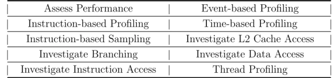
In our implementation, we leverage Intel’s VTunes [Reinders, 2005] on the In-tel architecture and AMD’s CodeAnalyst [Drongowski, 2008] (now CodeXL) on the AMD architecture. AMD implemented CodeAnalyst on both, Windows and Linux operating systems. CodeAnalyst provides a set of pre-defined profiling options to profile an application. Table 2.1 shows all of the options.
Assess Performance Event-based Profiling Instruction-based Profiling Time-based Profiling Instruction-based Sampling Investigate L2 Cache Access
Investigate Branching Investigate Data Access Investigate Instruction Access Thread Profiling
Table 2.1: Predefined Options to profile on AMD’s CodeAnalyst
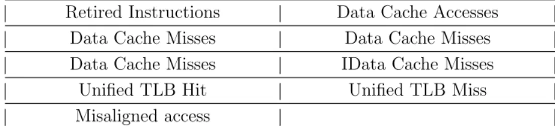
Each option mentioned in table 2.1 has a set of predefined events that the profiler will monitor on the HPCs. For example, the ‘Assess Performance’ profiling option presents a detailed analysis of system performance for the application under consider-ation [Drongowski, 2008]. The analysis includes a report on the instructions executed, the data & instruction cache accesses, the Translation Lookaside Buffer (TLB) hits & misses and Misaligned accesses in the main memory. To analyze such system features, HPCs monitor the following events, as shown in table 2.2.
pro-Retired Instructions Data Cache Accesses Data Cache Misses Data Cache Misses Data Cache Misses IData Cache Misses
Unified TLB Hit Unified TLB Miss Misaligned access
Table 2.2: Events profiled for Access Performance Profiling on AMD’s
CodeAnalyst
gram [Drongowski, 2008]. Hotspots are the maximum time-consuming phases of an application. The time-cost of a phase may be high due to potential memory bot-tlenecks, execution penalties or lack of optimization opportunities. To identify such hotspots, TBP tracks the following events, as shown in table 2.3:
CPU Clocks Instruction per Cycle Data Cache Miss Rate Data TLB L1/L2 Miss Rate
Misalign Rate Branch Mispredict Rate
Table 2.3: Events profiled for Time-based Profiling on AMD’s
Code-Analyst
It is important to note that the events mentioned in Table 2.3 are preconfigured and cannot be reprogrammed by a user. In TBP, CodeAnalyst configures a hardware timer that periodically interrupts the program executing on a processor core. The PMU samples the counters when a timer interrupt occurs. Post-processing in TBP aggregates the raw sample into a histogram for easy visualization of the profile.
Event-based Profiling (EBP) counts the number of hardware events occurred [Drongowski, 2008]. The PMU needs the following information to configure each counter with the specified event :
• An event count (sampling count)
• Choice of OS-space sampling, user-space sampling, or both • Choice of edge- or level-detect.
PMU will use the above set of information to configure an event on one of the coun-ters in the HPCs. Once the profiling starts, the kernel interrupts the counter as soon as the count for an event reaches the specified sampling count. In EBP, there are no preconfigured events. A user can choose any events from the pool of events provided by the family of the processor. For examples, on the Intel machine the available events to monitor depend on the microarchitecture (such as Nehalem, Haswell, and Skylake) of the processors [Intel, 2011].
For our application, we need features from both, TBP and EBP; i.e., the capa-bility of firing an interrupt once a timer is expired and the flexicapa-bility to monitor any desired event. This flexibility provides an opportunity to identify the top events that can predict the functional behavior of a program. Additionally, we desire to read the samples after a given sampling frequency, rather than sampling the HPCs after an event count has reached a certain sampling count. We impose such restriction because our malware detector demands a time-series of the count of occurrence of the architectural event. For example, suppose we monitor misaligned accesses with sampling count set as 1000 sample/second. The sampling count entails that the pro-filer will fetch the count of the number of misaligned accesses occurred once every millisecond. To facilitate profiling hardware performance events in the time domain, we introduce Savitor.
2.2
Savitor
Savitor is a HPC-based profiler implemented on Windows OS. A user can deploy Savitor on an AMD-based processor with any microarchitecture (such as Bulldozer and Athlon). As mentioned in section 2.1, the profiler features profiling of an ap-plication in the time-domain. Savitor uses AMD’s CodeAnalyst APIs [Drongowski, 2008] at the back end. The CodeAnalyst APIs provide a kernel level functionality to configure the HPCs with a desired set of event and then sample the configured events with a specified sampling frequency. With Savitor the sampling rate can be as fast as 3000 samples per second. The front end of the profiler is an user-interface to provide different profiling options to the user. These options include:
• Provide the hardware eventsto monitor on the HPCs. The number of events inputted can range from 1 to the number of hardware counters available per core on the architecture.
• The sampling frequency. The sampling frequency determines the rate at
which the HPCs are interrupted to read the counter values
• The application to profile. The application can execute on command prompt
or could have a Graphical User Interface (GUI)
• The output file to store the sampled values. The samples are stored in
plain-text and hence can be directly be used for further analysis of the data
• Total timeto profile. The profiling stops when this timer expires, or the appli-cation terminates, whichever happens first.
One of the responsibilities of Savitor is to make sure that profiling of the appli-cation is not dependent on the presence of other system processes. To achieve this, we designed Savitor to leverage multithreading on the AMD processors. Each thread
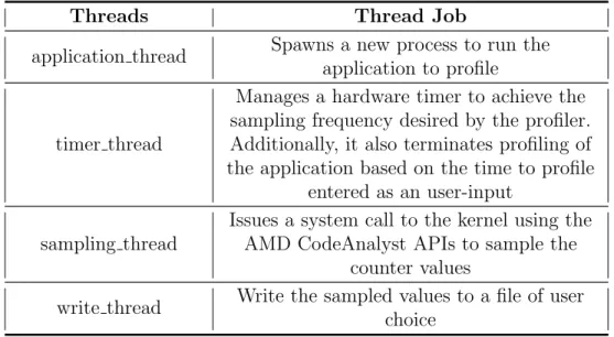
runs on a different core and is assigned a specific task. The first thread called the
application thread, spawns a new process with the application to profile. Savitor ex-ecutes all the process and the subprocesses of the application on the first core of the processor. The counting of the events on the HPCs occurs on a per-process basis. As a result, HPCs monitor only the threads of the processes or the subprocess of the application. Forcing an application to run on a single core enables the counters from that core to capture the entire execution profile sequentially; else, the profiles of mul-tithreaded applications will not capture the correct time sequence of the occurrence of the events. Additionally, in a multi-threaded computing system, the resources are shared amongst the processes running on the system. A scheduler manages the scheduling of these processes. The scheduler assigns a priority to each process, and higher priority processes usually get more resource usage time. Since it not possible to alter the current scheduler implementation on Windows OS, Savitor sets these threads to maximum possible priority-THREAD PRIORITY TIME CRITICAL be-longing to the REALTIME PRIORITY CLASS [Center, 2017] on the Windows OS. By assigning the highest priority, we ensure minimum preemption of the application’s processes (and their threads) by other user-level processes. Only OS-spawned threads can preempt the application’s processes. The second thread called the timer thread
is responsible for keeping track of time of profiling. Recall that, the user provides a time in second to profile each application. After the time expires, Savitor termi-nates both the profiling of the application. Thetimer thread runs on the second core. This thread also manages a hardware timer. This hardware timer determines the sampling frequency of the profiles. Once the timer expires, an interrupt is sent to Savitor, asking to read the counter values. A third thread called thesampling thread, on receiving an interrupt from the timer thread, uses the CodeAnalyst APIs to read the counter values. Additionally, the sampling thread also fetches the timestamp at
which the kernel sampled the HPCs. The next thread called the write thread gets the counts from the sampling thread and writes it these sampled counts from the HPCs to the file specified in user-input. The write thread logs the counts is -
times-tamp:event:count. The table 2.4 summarizes the job distribution of each thread in
Savitor.
Threads Thread Job
application thread Spawns a new process to run the application to profile
timer thread
Manages a hardware timer to achieve the sampling frequency desired by the profiler. Additionally, it also terminates profiling of the application based on the time to profile
entered as an user-input sampling thread
Issues a system call to the kernel using the AMD CodeAnalyst APIs to sample the
counter values
write thread Write the sampled values to a file of user choice
Table 2.4: Task List of the threads in Savitor
In principle, the sampling of the HPCs and the writing of the sampled values to a file are sequential tasks, even though Savitor assigns the two steps to two different threads. This is because, unless the sampling thread fetches the count value, the
write thread cannot log the counts into a file. On the other hand, the until the
write thread finishes writing the samples to the output file, the sampling thread has to hold the next fetched samples. To parallelize this process, we use a queue in the memory to hold the samples from the HPCs temporarily. As soon as thetimer thread
issues an interrupt to thesampling thread, thesampling thread fetches the timestamp from the kernel and the counts from the HPCs. The sampling thread pushes the timestamp, the sampled counts and the event monitored to the queue. This process is
repeated at the rate of the sampling frequency specified by the user. Thewrite thread
pops the three data fields (timestamp, events to monitor and the sampled counts) to log and write them to an output file. Using the queue, the sampling and the writing process are isolated. The queue is protected by a mutex to prevent pushing and popping elements from occurring at the same instant. Parallelizing the process of sampling the HPCs and writing the sample to the thread helped us achieve high sampling frequency of 3000 Hz.
2.3
Benignware and Malware Used
In our dataset, we profile 83 malware and 64 benignware. For benignware, we profile applications and services that are commonly used by consumers. We use the Future-marks PCMark [NIEMEL, 2005] benchmark suite to profile applications running on a Windows machine. PCMark classifies its benchmarks into:
• Essentials • Productivity
• Digital Content Creation • Gaming
We use the benchmarks from the ‘Essentials’ and ‘Productivity’ class. The Essential workload includes benchmarks like web browsing, one-to-one video calls, and video Conferencing. The Productivity workloads include spreadsheets and other writing related applications. We do not use benchmarks from the Digital Content Creation and Gaming class because of the workloads in these groups test GPUs extensively. On the other hand, we also profile web-based applications as benignware. In July 2017, a survey from Netcraft [Netcraft, 2017] received responses from 1,767,964,429 sites from 6,593,508 web-facing computers. The study highlights the large consumer-base of web users. According to a recent survey from PyCharm [PyCharm, 2016], 38% of web de-velopers, use Python for web development. Another survey from PyCharm [PyCharm, 2016] shows Django is most popular web framework used by Python developers. The numbers motivate us to use the services provided by Django as our benignware. To explore further, we also include services from Tornado in our setup. Additionally, we add a few features from SQLite to profile SQL-based applications. Table 2.5 shows some of the services that we profile on the HPCs. Web-Based applications commonly use one or more of these services.
chameleon chaos crypto pyaes django template regex effbot dulwich log unpack sequence fannkuch float genshi go regex v8 hexiom unpickle
hg
startup html5lib
json
dumps json loads r ichards logging
unpickle list mako meteor
contest nbody nqueens scimark pathlib
unpickle pure python pickle pickle
dict pickle ist pidigits spambayes pyflate xml tree python startup python startup no site raytrace regex compile spectral
norm regex dna
tornado http sqlalchemy declara-tive sqlalchemy impera-tive sqlite
synth sympy telco
Table 2.5: Django, Tornado and SQLite services used as benignware
For malware samples, we used the VirusTotal [Total, 2012] database to search for all the malware with the following tags:
• File OS - Win32
• File Type - Win EXE
• Machine Type - Intel 386 or later, and compatibles
• Subsystem - Windows CMD
These tags are important to make sure that we can run the malware samples via a command prompt on a 32-bit Windows 7 machine. The use of command prompt to execute an application aids in automating the profiling of the malware samples. Thus, we do not consider any malware samples whose subsystem is ‘Windows GUI.’ Our samples include a mix of malware such as worm, virus, and rootkits.
2.4
Feature Extraction
Feature extraction aims at extracting informative, non-redundant, and low-dimensional features from the HPCs. Each HPC-based profile is a multidimensional time series of the hardware events monitored on the HPCs. The raw samples collected from the HPCs cannot be used directly to train on the ML classifiers because the execution time being different for any application results in a different number of samples recorded across such applications. The inconsistency in the number of samples recorded by the HPCs will lead to each profile in our dataset to have a distinct dimension. Only an equidimensional dataset will facilitate comparison amongst the profiles. It thus becomes a hard requirement for each sample in the dataset to be equidimensional. To achieve an equidimensional dataset, we aggregate the raw samples from the HPC’s into 32 binned-histograms and then normalize the bins. Each bin is an aggregation of the number of samples recorded in a given time interval. The time interval is deter-mined by the number of bins. Thus, histogram gives the probability distribution of the occurrence of an event across the application’s entire execution time. Moreover, the aggregation of raw samples decreases the sparsity of our dataset. The sparsity of a matrix is the ratio of the number of zero elements in the matrix to non-zero ele-ments [Golub and Van Loan, 2012]. Depending on the data set, sparsity may reduce the information content of the dataset. In our case, a sparse data set comprising of the profiles from the HPCs indicates low or no occurrence of the corresponding event. A low count of a hardware event across the data set reduces the discriminating power of that event. Aggregating the samples into histograms increases the bin value of the bins by decreasing the number of zero elements in the dataset.
Additionally, during the execution of an application, the application behavior can differ substantially. As a result, the profile of each application shows inconsistent
vari-ation across the execution profile. For examples, assume that we measure L1-Data Cache Hits to profile an application. During the entire execution of the application, the number of L1-Data Hits can vary extensively based on the number of memory accesses made by that application. The inconsistent variation in the profile makes our data non-normal. In such situations, the ML classifiers with Gaussian kernel functions (such as SVMs and Gaussian Process) [G¨artner, 2003] show a bias towards features with more variation than the features with least variation. Gaussian kernels measure the Euclidean distance between the features in the dataset [Vert et al., 2004]. Intuitively, a strong statistical analysis of a data favors a perfect bell-shaped curve (normal distribution). Figure 2·1 shows a non-normal curve and a normal curve. To transform our dataset from non-normal distribution to a more approximate normal distribution, we use Power Transform.
(a) (b)
Figure 2·1: Variation in dataset: (a) A non-normal distribution #1;
and (b) Normal (Gaussian) Distribution #2. [University of Minnesota, 2017]
2.5
Feature Selection
HPCs on both Intel and AMD architectures provide over 200 architectural events. The ideal number of events to monitor simultaneously on the HPCs is equal to the number of counters present on each core in the architecture. As mentioned in section 1.4, we can monitor any number of events on the HPCs while the PMU will sample these events in a round-robin manner. Multiplexing multiple events will reduce the sampling frequency of the profiler, which affects the prediction accuracy of the ML classifiers. Subsequently, we monitor six events simultaneously on our AMD machines and four events on the Intel machines.
While training the ML classifiers, we consider each bin in the profile as a feature. The facility to monitor a large number of architectural events increases the number of potential features that can be used to train the ML classifiers. On the Intel and AMD machines, we can monitor 600 and 200 events respectively. On the other hand, the number of counters in each architecture usually ranges from four (like in Intel’s Nehalem microarchitecture) to eight (like in Intel’s Haswell microarchitecture and AMD’s Bulldozer). We thus need a feature selection algorithm to select the best events from the pool of all the available hardware performance events. Note that, any number of events can be extracted using our feature selection algorithm.
Additionally, if each bin is considered a feature, then each event contributes 32 features in the dataset (since each event is a vector of 32 binned histogram). As a result, the total number of features in the dataset will be equal to 128/192/256 for 4, 6 and 8 events monitored simultaneously. A dataset with a large number of features and low training examples may cause the problem of over-fitting [Hawkins, 2004] and train on the ML classifiers inefficiently. Secondly, the storage cost of the
data set during the training phase increases with the increase in number of features. To estimate the memory requirements by our implementation, we observed that our file was somewhere around 512 KB in size. In this scenario, each file stores traces for an event monitored on the HPC for an application executing for a minute. An application that is profiled using 8 events then requires 4 MB of memory. If we profile 1000 application on a system, the profile will take 4GB of space. This cost scales based on the number of applications in the dataset. The problems mentioned above while using a large number of features calls for decomposition of the data set using Principal Component Analysis (PCA). PCA yields the following advantages:
• Dimensionality reduction makes the dataset easier to comprehend by re-searchers/ users
• Shorter training times on complex classifiers such as SVM with RBF kernel • Dimensionality reduction avoids the curse of dimensionality [K¨oppen, 2000] • Enhanced generalization by reducing over fitting of the samples while training
the ML classifiers
As mentioned in the section 1.4, PCA divides a multivariate dataset into compo-nents that are linearly uncorrelated. To choose the top events, we first run a small dataset of 10 benchmarks on both Intel and AMD machines for all the events possible. We discard events that yield no samples for one or more applications in our dataset. Next, we create datasets comprising of the profiles of each event. We apply PCA on the datasets of the events, individually. The results from the PCA yields the per-centage of variance explained by each component. Intuitively, we want high variance ratio explained by each component. To this end, we sort the events in the order of the variance explained by each component. Our best events show a total of more
than 99% variance in the first two components itself. To this end, we chose the top four events for the Intel machine and six events for the AMD machines. The number of events chosen is in correspondence to the number of physical counters available on each core. For training our ML classifiers, we use the eigenvalues of the first two principal components of each of the chosen best events to obtain the transformed data points as our features. As a result, we have reduced a 128/192/256 dimensional to an 8/12-dimensional dataset on Intel and AMD machines respectively. Additionally, PCA minimizes the redundancy in our dataset.
2.6
Machine Learning Classifiers
In our implementation, we explore twelve classifiers to estimate their potential for malware identification. The classifiers are trained to behave as binary classifiers. The two classes are Malware and Benignware. We start training our dataset with linear algorithms like KNN and SVM( Linear Kernel). Additionally, we also use com-plex classifiers like SVMs (with Poly and RBF kernels), Decision Trees and Random Forests, MLP, AdaBoost and Logistic Regression. Table 2.6 gives a complete list of the classifiers used in our experimental setup. We use scikit-learn [Pedregosa et al., 2011] machine learning tools to train our classifiers. We follow use the 70-30% split to train our classifiers, i.e., 70% of the samples for training and the remaining 30% for testing. We cross-validate our results using k-fold cross-validation [Refaeilzadeh et al., 2009] technique with k = 10.
K Nearest
Neighbors Decision Trees Random Forest Naive Bayes SVM Linear SVM Poly SVM RBF SVM Sigmoid
Gaussian Process Logistic Regression AdaBoost MultiLayer Perceptron
Chapter 3
Evaluation
3.1
Experimental Setup
The end goal of this project is to test the capabilities of ML classifiers in differentiat-ing between benign and malicious HPC based profiles. We setup our experiments on Intel and AMD-based processor. For our Intel machine, we use the Intel I7-2600 pro-cessor which belongs to the Sandy Bridge microarchitecture and contain four physical counters per core. Additionally, the Intel machine had 4GB of RAM, private L1/L2-cache, and a shared L3-cache. For the AMD machine, we use the AMD FX-8150 processor which belongs to the Bulldozer family of processors. A bulldozer microar-chitecture has six physical counters per core. Each machine had 8GB of RAM, a private L1-cache and shared L2-cache. Our experimental setup uses 32-bit Windows 7 OS. The main motivation for using Windows is the existence of a large dataset of malware developed over the years.
The presence of other processes can affect the profiles collected by the HPCs since all the processes share the same hardware resources of the processor. We make sure that do not execute any other application in parallel to the application needed for profiling. Therefore during profiling, only the processes spawned by the application, the profiler and the OS are scheduled. Further, we run each application for 32 times on the same machine. Here, the motivation is to analyze the reproducibility of an HPCs based profile.
We ensure that the malware samples are successful in executing their malicious behavior by taking the following steps - we turned off both the Windows firewall set-tings and the Windows Defender1. Additionally, we did not have any third-party AV software installed on our system. To select top malware samples, we ran a preliminary test on the AMD machine, with randomly downloaded 1000 malware samples. We then time the execution of each malware sample and create a subset of all the malware samples that terminate within a minute of execution. We profile this subset of mal-ware samples on the HPCs using AMDs CodeAnalyst profiler. AMDs CodeAnalyst features an option of monitoring %CPU utilization and %Memory Utilization while executing a certain application. The motivation was that irrespective of the malware behavior, it is bound to use some CPU resources and some memory (at the least, the instruction memory). We ranked the Malware in the decreasing order of %CPU Utilization and %Memory Utilization in the first minute of the malware execution.
Potentially a malware can entirely or partially compromise the OS it is running on. To prevent profile creation on a faulty OS, we restore a clean copy of the OS after every single execution of malware. We divide our hard disk into two partitions; one partition has Windows 7 running all the benignware and malware. The second parti-tion has Ubuntu 16.04 LTS running on it. The Linux partiparti-tion stores a clean image of the Windows partition. After every single run of malware, on the Windows partition, the Linux partition restores the affected Window’s partition with the original clean image. To automate the above process, we modify the Linux GRUB bootloader to alternate booting into the two partitions on every restart. A restart signal is sent to the Windows operating system after the execution of the malware completes or after a minute, whichever happens first. As a result, the HPCs definitely monitor complete
or partial malware activity in the first minute of execution. After booting into the Linux OS, a startup script restores the fresh copy of the Windows image into the partition and then sends the power off signal with the restart option. The GRUB bootloader will now boot into the Windows partition. Figure 3·1 provides the cycle followed by the experimental setup to profile malware using HPCs.
Figure 3·1: Executing and Profiling Malware using Savitor and Intel’s
VTunes
The implementation stated in the above two paragraphs, i.e., running each ap-plication sequentially, and restoring a clean copy of the Windows while executing malware - causes a substantial increase in the total time to profile all applications in our dataset. The total time to profile a single run of malware takes ≈ 6 minutes to profile. To parallelize the profiling of the applications we create a cluster of the Intel and AMD machines with each machine in the cluster having the exact same hardware and software specifications. The Intel cluster has 12 nodes while the AMD cluster
has 21 nodes. Note that the number of nodes does not hold any importance in our implementation. Each cluster has a master node that is responsible for scheduling the profiling task on the slave nodes. The master node uses RabbitMQ [Videla and Williams, 2012] for scheduling the jobs to the slave nodes. RabbitMQ is an open-source message broker that can schedule tasks from a master entity to the available clients. Each slave node, after booting into the Windows partition informs the master of its availability to profile an application. The master node then responds to the slave with the next application to be scheduled.
On the AMD machines, we use Savitor to profile the applications. We set the sampling frequency to 1000 Hz, and monitor six events simultaneously. On the Intel machines, we use VTunes. On Windows 7 32-bit version, VTunes only provides com-mand line interface for measuring hardware performance events. In our experiments, we used runsa mode in VTunes, which records all the samples in the configured fre-quency. Even on the Intel machines, we set the sampling rate to 1000 Hz. After sampling the HPCs, we use VTunes report to extract the data into 32 bins with iden-tical time intervals during the one-minute experiment. The profiles from the HPCs are compressed using the Principal Component Analysis to eight components on the Intel machine and 12 components on the AMD machine. Each event contributes two 1 features in our dataset, and the Intel’s SandyBridge and AMD’s Bulldozer archi-tecture have four and six physical counters respectively. Table 3.1 summarizes the experimental setup described in this section.
Specifications AMD Setup Intel Setup
Processor AMD FX-8150 Intel I7-2600 Microarichitecture Bulldozer (Family
15h) Sandy-Bridge
RAM Size 8GB 4GB
OS Windows 7 32-Bit Windows 7 32-Bit Partition Loader OS Ubuntu 16.04 LTS Ubuntu 16.04 LTS
#HP Counters 6 4
Profiler Savitor Intel VTunes
Sampling Frequency 1000Hz 1000Hz
Feature Size (Post-PCA) 12 8
Cluster Size 21 15
3.2
Results after Feature Selection using PCA
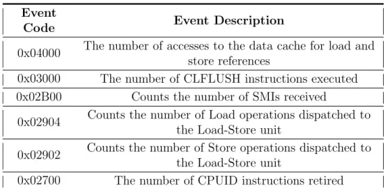
Table 3.2 and 3.3 show the top four and six events selected for the Intel and AMD experimental setups. These events show more than 99% of variance in their top two components.
Event
Code Event Description
0x04000 The number of accesses to the data cache for load and store references
0x03000 The number of CLFLUSH instructions executed 0x02B00 Counts the number of SMIs received
0x02904 Counts the number of Load operations dispatched to the Load-Store unit
0x02902 Counts the number of Store operations dispatched to the Load-Store unit
0x02700 The number of CPUID instructions retired
Table 3.2: List of Top 6 AMD Events Code & Description
Event Code Event Description
L2 LINES OUT
DEMAND DIRTY Dirty L2 cache lines evicted by demand LOCK CYCLES
SPLIT LOCK UC LOCK DURATION
Cycles in which the L1D and L2 are locked, due to a UC lock or split lock
FP COMP OPS EXE SSE PACKED
SINGLE
Counts number of SSE single precision Floating Point scalar uops executed L2 LINES OUT PF
DIRTY Dirty L2 cache lines evicted by L2 prefetch
Table 3.3: List of Top 4 Intel Events Code & Description
To analyze the result of PCA, we can either use a Scree Plot or a Cumulative Variation plot. The ideal pattern in a scree plot is a steep fall curve, followed by
a bend and then a flat or horizontal line. We retain those components