Crime and Victimization:
An Economic Perspective
W
hy is there more crime and violence in some countries than in others? And why is violent crime rising so rapidly around the world? What groups of people are most at risk from various types of crime? What evidence do we have that “crime waves” exist? Does poverty lead to high rates of violent crime? Or is it income inequality? Should crime alleviation be added to the list of benefits from economic reforms that generate sustained growth? Is the pro-cyclical nature of pub-lic expenditures in most developing countries exacerbating crime waves? Is education the key to solving the crime problem? How effective is police presence in fighting crime? Do people trust the police and judiciary? Are cultural and sociological factors overriding determinants of crime rates? Or are they secondary to economic forces? In particular, what makes Latin America one of the most crime-prone regions in the world? These ques-tions are of vital importance to policy makers. Although we can not pro-vide definite answers to all these issues, this paper should contribute to understanding them better and approaching their solutions.The incidence of crime and violence varies widely across nations and regions of the world. Notwithstanding the enormous heterogeneity in the levels of crime and victimization rates, there are signs that over the past decades the problems of crime and violence have worsened considerably
219
P A B L O F A J N Z Y L B E R D A N I E L L E D E R M A N N O R M A N L O A Y Z A
Fajnzylber is with the Universidade Federal de Minas Gerais. Lederman is with the School of Advanced International Studies, Johns Hopkins University. Loayza is with the Economic Research Group, Banco Central de Chile.
We are grateful to our conference discussants, Alejandro Gaviria and Peter Reuter, for their thoughtful comments. We also thank Roberto Steiner and Andrés Velasco for valuable suggestions and encouragement in the preparation of this paper.
throughout the world. Crime rates in industrialized countries have in-creased by 300 to 400 percent since the late 1960s.1From the early 1980s to the mid 1990s, the rate of intentional homicides increased by 50 percent in Latin America and sub-Saharan Africa and by more than 100 percent in eastern Europe and central Asia.2
The recent upward trend in crime rates has spurred widespread public concern about issues related to crime and insecurity, which in many coun-tries now attract more attention than traditional economic issues such as unemployment, inflation, and taxes. In the United States, public opinion polls conducted in the mid-1990s reported violent crime as the nation’s “most serious problem.”3In England and the Netherlands more than half of the public see crime as the number one problem facing their country, while in France 39 percent place it at the top of citizens’ concerns.4Similar con-clusions can be derived from polls conducted in seventeen Latin American countries in 1996, which describe violence as “the region’s main social and economic problem.”5
This paper examines the main issues concerning crime and victimiza-tion from an economic perspective, combining a review of the main results established in the literature with original research on the causes of crime and the risk factors of victimization. The following section provides an overview of the costs and causes of crime, together with a brief look at the type of data available for analyzing crime. We start by presenting the main methodological approaches for measuring the costs of crime and pres-ent estimates for selected developed and developing countries. We then survey the literature on the causes of crime, which extends from Becker’s original contribution to the recent developments that emphasize social interactions. The survey covers both theoretical results and empirical evi-dence, emphasizing how the interaction between the two has stimulated their development. Finally, the section on crime data describes the main sources of information regarding crimes, victims, and offenders, and it dis-cusses the relative advantages of crime statistics derived from official sources and from victim and offender surveys.
1. International Centre for the Prevention of Crime (1998, chap. 3, p. 5). 2. Fajnzylber, Lederman, and Loayza (1998, pp. 11–15).
3. New York Times and CBS poll, quoted in Blumstein (1995, p. 10). 4. International Centre for the Prevention of Crime (1998, chap. 3, p. 2).
The next section presents original work on the main causes of violent crime from a cross-country perspective. The objective of this section is to analyze the social and economic determinants of homicide and robbery rates (at a national level) in a worldwide sample of countries. We start with an empirical model in which the main determinants of violent crime rates are economic variables. This basic model includes as explanatory variables the average and distribution of national income, the growth rate of out-put, the average educational attainment of the adult population, and the lagged crime rate (to allow for inertial effects). In turn, we extend the basic model along five dimensions: (1) deterrence factors, (2) activities related to illegal drugs, (3) demographic issues, (4) income and ethnic polariza-tion, and (5) social capital.
The paper then reviews the empirical evidence from recent Latin Amer-ican case studies that rely on household or individual victimization surveys conducted in major urban centers in the late 1990s. In the final section we phrase our main results in terms of policy implications. Thus we attempt to show how the conclusions of the paper can form the basis for specific policy recommendations.
A Review of the Costs, Causes, and Data Sources on Crime
This section provides an overview of some conceptual issues regarding the costs of crime, together with available estimates; theoretical and empiri-cal research on the causes of crime and violence; and the relative advan-tages of official crime statistics versus victimization surveys.
The Costs of Crime
The concern with crime is well justified given its pernicious effects on eco-nomic activity and, more generally, on the quality of life of people who must cope with a reduced sense of personal and proprietary security. Sev-eral approaches have been used to measure the social costs of crime, and estimates vary considerably depending on the adopted methodologies and assumptions.
The simplest way is to adopt an accounting perspective and add up all the direct and indirect losses from crime. Lack of appropriate data and disagreements on the specific assumptions about the opportunity costs of
the lost resources constitute the main limitations to this type of calculation. The most common categories considered in the accounting of the costs from crime include the amounts spent on policing, courts, and prisons; private security expenditures; the value of potential years of life lost due to murder or crime-related disabilities; and the health-care costs associated with traumas caused by violence (when they do not result in death or dis-ability). Crime also leads to other indirect costs that are more difficult to quantify. Complete estimates should include the discounted value of stolen property (see below), the underinvestment that crime causes in the legal sector, the reduced productivity of businesses, reductions in the rates of human and social capital accumulation, the lowering of labor force partic-ipation rates, and the intergenerational transmission of violent behaviors.6 Since many stolen goods are not lost to society as a whole but are instead transferred from victims to criminals, it is not obvious that the total value of those goods should be accounted as a social cost. Since the value of stolen property is potentially smaller for the criminals than for the vic-tims, one could argue that only the difference between these two valua-tions should be taken into consideration as a welfare loss. However, as Glaeser emphasizes, given that the time spent by criminals in illegal rather than legal activities is in fact a social loss and since the value of goods taken should in equilibrium be equal to the opportunity cost of the crimi-nals’ time, all property losses should be considered social losses.7
Estimates performed in industrialized countries indicate that the costs of shattered lives account for the largest share of all measured crime costs: in Australia, England, France, and the United States, the value of lost lives represents more than 40 percent of those costs.8In the specific case of women, every year 9 million years of healthy lives are lost worldwide as a result of rape and domestic violence.9This loss is larger than the corre-sponding loss due to all types of cancer in women and twice as large as the loss due to motor-vehicle accidents suffered by women.10
In the United States, a study using 1992 data estimated that crime caused a loss of $170 billion in the form of suffering and potential years of life lost, while public expenditures on the criminal justice system and
pri-6. See Buvinic and Morrison (1999, technical note 4). 7. Glaeser (1999, p. 19).
8. International Centre for the Prevention of Crime (1998, chap. 2, p. 3). 9. World Bank (1993).
vate security costs amounted to $90 billion and $65 billion, respectively.11 Adding these figures to the value of lost jobs due to urban decay ($50 bil-lion), property losses ($45 bilbil-lion), and treatment of crime victims ($5 billion), this study estimated the total cost of crime to be $425 billion per year. This represents more than 5 percent of the U.S. gross domestic product (GDP). Similar figures were obtained using analogous proce-dures in Australia, Canada, and the Netherlands.12
In Latin America, a recent study conducted at the Inter-American Development Bank (IDB) estimates that the social costs of crime, includ-ing the value of stolen properties, amount to $168 billion, or 14.2 percent of the region’s GDP.13The largest cost category in this study is that of intangibles, which accounts for half of the estimated costs of crime. This category includes the effects of crime on investment and productivity (esti-mated on the basis of unspecified time-series or cross-country economet-ric models) and the impact on labor and consumption (as measured, in unspecified surveys, by the citizens’ willingness to pay to avoid violence). One could argue that the very high intangible costs from crime found in Latin America are the result of the region’s higher levels of crime, possibly coupled to a non-linearity in the relation between crime and its impact on citizens’ welfare. That is, the pernicious effects on the quality of life may in fact accelerate when crime rates cross some threshold level.14It is also theoretically plausible that crime produces diminishing welfare effects as its incidence rises. Alternatively, the higher Latin American estimates of so-called intangible costs may stem from methodological differences or from the sensitivity of the results to the quality of the available data.15
11. Mandel and others. (1993).
12. International Centre for the Prevention of Crime (1998, chap. 2, p. 3). 13. Londoño and Guerrero (1999, p. 27).
14. Alternatively, in explaining the intangible costs of crime, the cumulative effect of relatively high levels of crime over a long period of time may be more important than the levels of crime at a given point in time. Thus the costs of crime could grow even in the context of stable or declining crime rates.
15. An approach that has not been applied to date in Latin America is that of using so-called hedonic estimates of housing prices to measure the economic costs of crime. In the United States, results from studies of this type indicate that a doubling of crime rates could lead to a reduction of 8 to 12.5 percent in real estate costs (Buvinic and Morrison, 1999). One advantage of these studies is that they generate estimates of the value of marginal reductions in the level of crime, as opposed to accounting estimates of the total costs of crime (Glaeser, 1999, p. 20). Indeed, the former may be most useful from a practical point of view, since most policy measures will not lead to a complete eradication but rather to mar-ginal reductions of the level of crime.
If one excludes intangibles and the value of stolen goods (about $25 bil-lion dollars), the remaining social costs of crime still amount to 4.9 percent of Latin America’s GDP, with the largest category being the cost of poten-tial lives lost and other health-related costs (1.9 percent of the region’s GDP), followed by expenditures on police and the criminal justice sys-tem (1.6 percent of GDP) and the cost of private security (1.4 percent of GDP).16The IDB estimates demonstrate considerable differences across countries. While Mexico stands close to the region’s average, with crime costs (excluding intangibles and transfers) of 4.9 percent of GDP, crime in El Salvador and Colombia lead to losses of 9.2 and 11.4 percent of GDP, respectively. At the other end of the spectrum, crime-related costs in Peru and Brazil amount to 2.9 and 3.3 percent of GDP, respectively.17
The very high social and economic costs of crime and violence indi-cate that these problems have become serious obstacles to sustainable social and economic development in many countries around the world. Moreover, the recent worrisome trends in crime rates have created a sense of urgency. Governments and international organizations now face the for-midable challenge of designing and implementing policies to prevent and reduce crime and violence. A necessary first step is to develop a better knowledge of the causes of crime and violence.
The Causes of Crime
At least since the pioneering work of Becker, economists have analyzed the determinants of crime from the perspective of the offender’s rational decision to participate in illegal activities, on the basis of a cost-benefit analysis.18In his Nobel lecture, Becker emphasized that the economic way of looking at human behavior is a “methodof analysis, not an assumption about particular motivations, . . . [which] assumes that individuals maxi-mize welfare as they conceive it . . . .”19Regarding issues of crime and
punishment, Becker writes that this rationality implies that “some indi-viduals become criminals because of the financial and other rewards from crime compared to legal work, taking account of the likelihood of appre-hension and conviction, and the severity of punishment.”20Below, we
16. Londoño and Guerrero (1999, p. 22). 17. Londoño and Guerrero (1999, p. 26). 18. Becker (1968).
19. Becker (1993, pp. 385–86, emphasis in original). 20. Becker (1993, p. 390).
review some of the main contributions to the economics literature on the determinants of crime, which has developed considerably in recent years, particularly in the United States.
One of Becker’s main insights is that criminal behavior responds to changes in expected punishment. This assertion has received consider-able empirical support dating back at least to the 1970s. This evidence has been based on econometric analysis of the effects of expected punish-ment on crime, using cross-sectional and time-series data at the level of states, cities, and neighborhoods, while controlling for a number of other factors. In early studies of this sort, Ehrlich estimates the elasticity of crime with respect to the expected size of punishment to be −0.5, while Mathieson and Passell calculate it at −0.3.21Using data on capital
punish-ment provisions across the United States, Ehrlich finds that the death penalty has a major impact on crime rates.22
Analysts often make a subtle distinction between deterrent effects, which are associated with policing and convictions, and incapacitation or preventive effects, which result from locking up (or killing, in the case of capital punishment) criminals who have a tendency to rejoin the crime industry once they are released. As Ehrlich states, “deterrence essentially aims at modifying the ‘price of crime’ for all offenders while incapacitation —and for that matter, rehabilitation—acts through the removal of a sub-set of convicted offenders from the market for offenses.”23The empirical
evidence, at least for the United States, has favored the idea that impris-onment reduces crime rates mostly through deterrence rather than through incapacitation.24
An assessment of the effectiveness of deterrence must also incorporate individual attitudes toward risk, which affect the expected utility from ille-gal income. In principle, if individuals are risk neutral, increases in the probability of arrest and conviction and increases in the size of the penalty, conditional upon conviction, should have the same effect on crime. For risk-averse individuals, however, raising the probability of conviction may have greater deterrent effects than raising the severity of punishment.25The
21. Ehrlich (1973); Mathieson and Passell (1976). 22. Ehrlich (1975a).
23. Ehrlich (1981, p. 311).
24. Ehrlich (1975a, 1981); Levitt (1998a).
25. Becker (1968, p. 178); Ehrlich (1973, p. 528). The standard assumption in theoret-ical models is to consider individuals who are risk averse, but who exhibit decreasing risk aversion with increasing income (Schmidt and Witte, 1984, p. 161).
empirical evidence for the United States indicates that criminals may indeed be risk averse, as they respond more readily to increases in the probability of arrest than to increases in the time spent in prison.26
One serious econometric problem that afflicts most of the early empir-ical estimates of the relation between crime and punishment is that crime-reducing efforts through increased deterrence are usually not exogenous with respect to crime levels. High crime rates may induce governments to increase the number of police or the severity of the punishment. Thus, ordinary least squares (OLS) regressions of crime rates on deterrence variables may underestimate the crime-reducing effect of the latter, and they may even lead to spurious positive correlations between crime and deterrence.
Levitt greatly contributes to overcoming this problem by using econo-metric techniques aimed at isolating exogenous sources of variation in the level of deterrence.27By constructing variables that capture exoge-nous variations in the size of the prison population, the number of police per capita, and arrest rates, Levitt finds robust evidence that all these mea-sures of deterrence have significant effects on crime, as predicted by Becker’s economic model. In estimating the effect of prison populations on crime, Levitt corrects for the simultaneity bias arising from the fact that for a given probability and severity of punishment, the prison population should increase with the overall crime rate.28To this end, he uses the status of litigation on state prison overcrowding as an instrumental variable for the rate of change of incarceration rates.29Levitt’s estimates of the elas-ticity of crime with respect to prisoners are almost four times higher when the endogeneity of prison populations is controlled for. After taking into account a number of economic and demographic crime determinants, Levitt finds that a 100 percent increase in the number of prisoners per capita causes a 40 percent reduction in violent crime rates and a 29 percent reduction in property crime rates.
26. Grogger (1991). This result is also supportive of the prevalence of the deterrent vis-à-vis the incapacitation effects of imprisonment.
27. Levitt (1996, 1997, 1998a). 28. Levitt (1996).
29. Prison overcrowding lawsuits have been filed in the United States since 1965 on the grounds of unconstitutional conditions in prisons. Levitt shows that the filing of prison overcrowding litigation leads to the lowering of prison population growth rates, even before the courts reach any decision. Moreover, the status of prison overcrowding litigation is shown to be unrelated to previous crime rates.
Following a similar approach, Levitt correlates changes in the number of police per capita with electoral cycles and then uses the variable to elicit the pure effect of policing on crime rates across cities.30Levitt shows that police forces in large U.S. cities grow disproportionately faster in mayoral and gubernatorial election years, while crime rates do not appear to be significantly related to electoral cycles, at least after controlling for other types of social spending and for economic conditions. Election-year indicator variables are thus used as instruments for the number of police officers. For six out of seven crime categories, this procedure leads to negative and significant estimates of the elasticity of crime with respect to the size of the police force. Additional controls are included to account for unobserved heterogeneity in levels and rates of change of crime rates, which could also positively bias the above elasticities. Results indicate that each additional police officer reduces the number of reported crimes by approximately eight per year. Using available estimates of the social costs of crime and the total costs of hiring additional police officers, Levitt concludes that police staffing in large American cities is below its optimal level.
Finally, Levitt turns to the negative relation between crime and arrest rates that is often found in empirical tests of the deterrence hypothesis, in order to determine whether this result supports this hypothesis or can instead be attributed to an endogeneity bias.31A bias could arise because the underreporting of crime leads to a measurement error in the number of reported crimes, which appear both in the numerator of crime rates and in the denominator of arrest rates. Levitt estimates the arrest-crime elasticity using first through fourth differences of both variables, expecting to find lower absolute values for the longer differences, given the fact that they should be less affected by measurement-error bias. The various esti-mates are not, however, significantly different from each other, which sug-gests that the bias resulting from measurement error is not substantial. The negative correlation between arrests and crimes is not spurious, but reflects either deterrence or incapacitation. To distinguish between these two effects Levitt estimates the effect of arrest rates for a specific type of offense on the rates of other crimes. Assuming that property and violent crimes are not substitutes for one another (that is, criminals would not
30. Levitt (1997). 31. Levitt (1998a).
switch from one to the other in response to changes in relative arrest rates), he interprets the corresponding cross-elasticity as reflecting exclusively an incapacitation effect. Using these estimates, in conjunction with published information on the time served per arrest and on the likelihood of re-arrest for each type of crime, Levitt estimates the deterrence and incapacitation components of the reduction in a given crime associated with increases in own-crime arrests. He concludes, as does Ehrlich, that deterrence is empir-ically more important than incapacitation. This is particularly true for assault and property crimes, for which deterrence explains a minimum of 75 percent of the overall effect. Still, incapacitation effects are not negli-gible: Levitt estimates that each additional person-year of incapacitation leads to a reduction of 5.1 to 8.2 index crimes.
A recent line of research questions the motives of officials in the police and judiciary. Law enforcement has traditionally been assumed to serve the needs of the people or to maximize some social welfare function, but researchers increasingly recognize that law enforcement officials respond to their own incentives, which are not always consistent with society’s welfare. This literature is still mostly limited to the United States. In a pio-neering article, Posner attempts to understand what it is that judges maxi-mize.32Glaeser and Sacerdote examine the factors that are associated with higher levels of punishment for murderers in the United States.33They find that people who kill African-Americans get shorter sentences, while mur-derers of women are more severely punished. These behavioral patterns presumably illustrate the attitudes of the judges who make most of these sentencing decisions. Glaeser, Kessler, and Piehl show that federal prose-cutors act decisively against criminals with more income and higher level of human capital.34They argue that this relates to the career ambitions of the prosecutors, who want to distinguish themselves by prosecuting high-profile criminals. If the issue of police and judiciary incentives is relevant in the United States, it is much more so in developing countries, where corruption and lack of accountability are endemic problems in the public administration.
The literature on the payoffs and opportunity costs of crime is also rich. Fleisher and Ehrlich were pioneers in studying the effects of income levels and
32. Posner (1995).
33. Glaeser and Sacerdote (1999b). 34. Glaeser, Kessler, and Piehl (1998).
income disparities on the incidence of crime.35Fleisher argues that the the-oretical effect on crime of higher levels of average income is a priori ambiguous, because both the opportunity cost and the expected payoff from crime are correlated with income. Fleisher’s and Ehrlich’s empirical findings about the effects of income levels are mutually contradictory.36 However, both authors find a significant crime-inducing impact of income inequality.37 Ehrlich’s interpretation of this result is that, for a given median income, larger income inequality is an indication of a larger absolute differential between the payoffs from legal and illegal activities.38 A number of studies focus on the relation between crime and labor mar-ket outcomes, such as employment and wages. Both Fleisher and Ehrlich examine the effect on crime of the unemployment rate, viewing the latter as a complementary indicator of income opportunities available in the for-mal labor market.39In their empirical studies, however, both authors find that unemployment rates are less important than income levels and distri-bution. Time-series studies have failed to uncover a robust, positive, and significant relation between unemployment and crime, but most studies based on cross-sectional and individual data do point in that direction.40 A recent study by Tauchen, Witte, and Griesinger uncovers a negative rela-tion between the amount of time spent working and arrest rates, using indi-vidual data on the Philadelphia birth cohort of 1945.41In another recent study with individual data, Grogger provides convincing evidence relating
35. Fleisher (1966); Ehrlich (1973).
36. Fleisher (1966) finds that a city’s average family income has a negative effect on the arrest rates of young males, while Ehrlich (1973) finds that states with higher median fam-ily incomes have higher rates of violent and property crimes.
37. Fleisher (1966) measures income inequality as the difference between the average income of the second lowest quartile and the highest quartile of households, whereas Ehrlich (1973) uses the percentage of families below one-half of the median income.
38. Ehrlich (1973) assumes that the median income for the state is a good proxy for the payoffs from crime—the “opportunities provided by potential victims of crime”— while legitimate opportunities available to potential offenders may be approximated by the mean income level of those below the state’s median income.
39. Fleisher (1966); Ehrlich (1973). In the words of Fleisher, “in attempting to esti-mate the effect of income on delinquency, it is important to consider the effects of both normal family incomes and deviations from normal due to unemployment” (1966, p. 121). 40. See the literature review in Freeman (1994). Two notable exceptions are Witte (1980) and Trumbull (1989). Trumbull’s analysis is based on county-level data from North Carolina, while Witte follows a sample of North Carolina men released from prison.
market wages to youth crime participation rates.42The author uses data from the U.S. National Longitudinal Survey of Youth (NLSY) to estimate a time-allocation model in which individuals choose how much time to allocate to legal and illegal work. His econometric results indicate that the drop in youth wages observed in the United States since the mid-1970s may explain as much as three-quarters of the rise in youth crime over the same period.43
Another important factor related to the effect of economic conditions on crime is the educational level of the population, which can determine the expected rewards from both legal and criminal activities. Criminals tend to be less educated and from poorer backgrounds than noncriminals: in 1986, over two-thirds of all eighteen- to twenty-four-year-old male prisoners and three-fourths of the eighteen- to twenty-four-year-old black male prisoners had fewer than twelve years of schooling. For the corresponding cohorts of nonimprisoned men, only 25 and 30 percent, respectively, had attained that educational level.44Thus one could expect that areas characterized by higher average educational levels should have a lower incidence of crime. Ehrlich reports, however, that property crime rates in the United States are positively and significantly related to the average years of schooling of the population aged twenty-five and over, even after controlling for income inequality and median income.45The author provides several explana-tions for this puzzling empirical finding: education may raise productiv-ity in illegal activities to a greater extent than in legal ones; higher aver-age levels of education may be associated with less underreporting of crimes and with wealthier potential victims; and higher average levels of education may go hand in hand with more pronounced educational inequities.46
In contrast, the evidence from studies based on individual data sup-ports a negative effect of education on crime. This effect is not necessar-ily derived from the greater legitimate income that is potentially associated with education, however, but rather from participation in legitimate
activ-42. Grogger (1997).
43. Grogger (1997). The author’s econometric results on the youth wage-crime rela-tion also help explain racial differences in rates of crime participarela-tion and the age distribu-tion of crime.
44. Freeman (1991, p. 6). 45. Ehrlich (1975b).
ities per se. Witte and Tauchen, for example, find that for a sample of young men, the act of going to school or work reduces the probability of committing criminal acts, even if a high school degree does not have a sig-nificant effect on that probability.47
In somewhat of a departure from Becker’s paradigm, an increasing number of studies turns to the sociological aspects of the incidence of crime. Dilulio argues that the prevalence of high crime rates in U.S. cities is related to the depletion of what social scientists call social capital.48 Putnam defines social capital as the “features of social organization, such as trust, norms, and networks, which can improve the efficiency of soci-ety in facilitating coordinated actions.”49Thus Freeman finds a strong rela-tion between church attendance and a lower probability of arrest for youth surveyed in the NLSY.50Glaeser and Sacerdote find that the most impor-tant explanation of urban crime rates in the United States is the percent-age of female-headed households, which is responsible for almost 30 per-cent of the city-crime effect.51
Similarly, individual perceptions of the benefits and costs of criminal activity are determined by their environment. Using a survey of disadvan-taged youths in Boston, Case and Katz find that an individual’s propen-sity to commit a crime rises when peers are also engaged in criminal activ-ities.52This empirical finding has been modeled by Glaeser, Sacerdote, and Scheinkman, who emphasize the role of social interactions in explaining the significant variance of crime rates across U.S. cities. They argue that both the cost of crime and the propensity for it are determined by local social interactions among criminals, their peers, and their family mem-bers.53An important implication is that crime rates across different cities need not converge.
47. Witte and Tauchen (1994). The same finding is reported in Tauchen, Witte, and Griesinger (1994, p. 410), who find a negative relation between crime and the variables for the amount of time spent at work and at school, but no significant effect from educational attainment on arrest rates. Moreover, the coefficients for the time spent at work and at school are not significantly different from one another. This finding is also present in Farrington and others (1986); Gottfredson (1985); Viscusi (1986).
48. Dilulio (1996, pp. 20–21). 49. Putnam (1993, p. 173). 50. Freeman (1986).
51. Glaeser and Sacerdote (1999a, p. S253). 52. Case and Katz (1991).
Sah emphasizes the role of another type of social interaction, this time operating at the macroeconomic or systemic level. Individuals living in areas with high crime participation rates may perceive a lower probabil-ity of apprehension than those living in areas with low crime participa-tion rates, because the resources spent in apprehending each criminal tend to be low in high crime areas. An important implication is that “past crime breeds future crime.”54Thus, as in the case of the social interactions mod-eled by Glaeser, Sacerdote, and Scheinkman, systemic social interactions may cause cities and countries to experience criminal inertia over time.
Two issues that have recently received special attention from econo-mists and other social scientists are the relation between crime and drugs and the explanation of youth crime participation. For instance, Blumstein shows that the homicide rate among youth aged eighteen and under, the number of homicides committed by juveniles with guns, and the arrest rate on drug charges among nonwhite juveniles all more than doubled between the mid-1980s and the early 1990s.55The same period saw no growth in the homicide rate among adults aged twenty-four and older and no growth in either the drug-related arrest rate for white juveniles or the number of juvenile homicides not involving guns. Blumstein attributes these worri-some trends to changes in the illegal drug market that were brought about by the introduction of crack cocaine. Because of its low price, crack cocaine attracted a larger number of buyers and led to an increase in the number of transactions. This, in turn, led to a considerable increase in the number of drug sellers, who are usually recruited among inner-city juve-niles because of their lower opportunity costs and because of the relatively lenient punishments they face when caught. Because most drug dealers carry guns for self-protection and because dispute resolution in the illegal drug market is often violent, the growth of the crack cocaine market was accompanied by an increased diffusion of guns among juveniles. This, Blumstein argues, led to a greater incidence of both drug- and non-drug-related lethal violence among youth.
Grogger and Willis provide statistical tests of the hypothesis that the introduction of crack cocaine led to significant increases in crime in twenty-seven U.S. metropolitan areas.56Given the fact that crack markets
54. Sah (1991, p. 1282). 55. Blumstein (1995). 56. Grogger and Willis (1998).
are mostly concentrated in inner cities, Grogger and Willis assume that crack cocaine had no effect on suburban crime rates. They then compare crime rates in inner cities and suburbs, as well as before and after the intro-duction of crack in each metropolitan area. Results suggest that most index crimes experienced significant increases after crack was introduced; the only nonsignificant increases are for burglary and rape. Grogger and Willis also report econometric estimates of the effects of the introduction of crack cocaine, after controlling both for economywide period effects that influ-ence crime rates differently in inner cities and suburbs and for area- and year-specific unobservable factors that may influence the introduction of crack. These results also favor the existence of sizeable positive, signifi-cant effects from crack introduction on violent crimes and robbery but not on other property crimes.
Grogger and Willis suggest that crack cocaine can be seen as a tech-nological innovation that reduces the unit cost of cocaine intoxication. It thus leads to an outward shift in the supply curve for this product, and consequently the number of drug transactions increases, as does the inci-dence of violence, which is viewed as the main tool for enforcing agree-ments in the presence of incomplete property rights. As for the finding that crack cocaine had almost no effect on the rates of property crimes, Grogger and Willis hypothesize that these crimes are related to the demand side of the market, as they provide users with the income they need to purchase the drug. If the elasticity of the demand for drugs is rel-atively low, as can be expected for habit-forming goods, the outward shift in the supply curve may lead to a reduction in the total expenditures in cocaine intoxication, which would explain the absence of effects on property crimes.
The decline in violent crime rates in the United States after 1991 has also been linked to the crack cocaine epidemic, which began to abate in the early 1990s.57Other factors have certainly contributed to that decline as well, such as the long period of economic expansion in the United States and the increase in incarceration since the mid-1980s. In any case, the recent swings in the homicide rates of the younger age groups have
57. Blumstein and Rosenfeld, (1998); Grogger (1999). Grogger (1999) argues that the costs of entry in the market for illegal drugs increased with the escalation of violence that accompanied the introduction of crack cocaine. This would have shifted the supply curve for illegal drugs upward, which would explain the reversal in drug-related violence.
certainly contributed to spurring interest in juvenile crime, especially in the extent to which young offenders are responsive to economic incen-tives. The available evidence suggests that this is indeed the case, both for positive and negative incentives.58
The economics literature on the causes of crime has thus moved from an emphasis on deterrence effects and economic conditions to more recent considerations of social factors that may help explain how crime is prop-agated over time and within communities. This evolution has been spurred by the continuous interaction between theoretical and empirical contribu-tions. The development of the latter, in particular, is highly dependent on the availability of appropriate sources of data, to which we now turn.
Data Sources on Crime
Empirical studies on the economic determinants of crime can take several forms and aim at different objectives, depending on the type of data they use. The data on crime can be classified according to their source, level of aggregation, and availability of longitudinal observations.
The most frequently used source of crime data is the criminal justice system. Official crime statistics can be tabulated at different levels of aggregation (for example, counties, cities, states, or countries) and allow for analysis based on time-series, cross-sectional, or even panel data. The main limitation of this source of data is that only a fraction of all offenses ever make their way into official statistics, which are commonly thought to underestimate the actual incidence of crime. This happens because victims frequently do not report crimes to the police, especially when minor offenses are involved, when victims do not have confidence in the local authorities, and when victims view the event as a private matter. The latter is most often the case when crimes involve interpersonal vio-lence (such as rape) and when offenders are known to the victims (as in domestic violence).59
Official crime data also suffer from deficiencies in the recording pro-cedures of the police and justice systems, which in many cases do not
58. Levitt (1998b) shows that juvenile crime is at least as responsive to criminal sanc-tions as is adult crime; Grogger (1997) shows that when deciding to participate in crime, youth do take into account the level of legitimate wages; and Mocan and Rees (1999) find that juvenile crime responds to arrest rates and to local economic conditions.
compute their statistics from the complete set of law enforcement agencies existing in each country. Moreover, the quality of official crime statistics may be jeopardized by the selectivity with which crimes are recorded by the criminal justice system: crime statistics could be measuring “the behavior of officials and not of crime.”60For example, in El Salvador the Fiscalía General de la República (the office of the country’s chief prose-cutor) only records crimes for which there is an indicted suspect.61
A second type of crime data involves homicide and intentional injury statistics collected from hospitals and morticians. These data are usually collected and tabulated by the countries’ health authorities and serve as an alternative, or complement, to the violent crime statistics collected through law enforcement agencies. Tabulations are available at several levels of aggregation, and usually in the form of time series.
Homicide data are of special interest because these crimes are usually thought to be the least affected by the problems of underreporting and underrecording that afflict official crime statistics. In cross-country stud-ies, the use of homicide data is further justified by the fact that they are less sensitive to changing definitions of crimes across legal systems. Even in the United States, experts have frequently focused on homicides as a proxy for crime, not only because “it is a fairly reliable barometer of all violent crime” but also because “at a national level, no other crime is measured as accurately and precisely.”62
Victimization surveys, which are the third source of crime data, are “the primary workhorse” for measuring crime.63These surveys are collected from city- or country-representative samples of households. They provide information about nonfatal crimes and have the main advantage of includ-ing incidents not reported to the police, as well as detailed information about victims, offenders, and criminal offenses. To be useful for analysis, victimization surveys must have geographic identifiers that enable the researcher to link the individuals to the community in which they live or were victimized. The researcher also needs a description of that commu-nity, which may be drawn from broader national surveys or national cen-suses. Victimization surveys are a relatively new source of crime data. In
60. Gottfredson (1986, p. 256).
61. Cruz, Trigueros Argüello, and González (2000, p. 14). 62. Fox and Zawitz (2000, p. 1).
the United States, the Bureau of Justice Statistics, in conjunction with the Census Bureau, has regularly performed such surveys since 1973. Other countries that pioneered this type of research are Canada, the Netherlands, and the United Kingdom. Since 1989, the United Nations Interregional Crime and Justice Research Institute (UNICRI) has been promoting the application of methodologically consistent city-level vic-timization surveys around the world. By 1998, these International Crime Victim Surveys (ICVS) had been performed in 55 countries.64
A final data source is the offender survey. This type of survey can be taken through traditional survey methods in which respondents are asked if they have been arrested (or less reliably, if they have committed a crime). Alternatively, these surveys can be done at the point of arrest or through surveys of prison populations, in which case it must be assumed that the police arrest a relatively random sample of the population of criminals. When this type of data set is merged with data on the population at large, it is then possible to identify how criminals differ from average citizens. This was the approach adopted by Glueck and Glueck, who are known as the pioneers of empirical research on crime in the United States.65These authors followed two matched samples of offenders and nonoffenders over many years and laid the foundations for most of the subsequent cross-sectional and longitudinal research in criminology.66
All in all, studies based on cross-sectional and panel data have been the most common, while studies exclusively using time-series data have been the less abundant. This is largely because time series of crime data are usually not available for long periods. However, time-series studies and studies based on panel data share some important advantages. Unlike cross-sectional studies, they allow researchers to establish cause and effect, “by showing that changes in one factor are followed by changes in another.”67 Moreover, the temporal variation in the data allows the researcher to consider the effects of the business cycle on crime, as well
64. Newman (1999, p. 25).
65. Glueck and Glueck (1950, 1968).
66. Gottfredson and Hirschi (1990, p. 221). Cruz, Trigueros Argüello, and González (2000) use prison survey data to study the factors that make some criminals more violent than others.
67. Farrington (1986, p. 212). Panel data also provide the researcher with a means of controlling for reverse causality and other sources of endogeneity in the explanatory variables.
as to test the hypothesis of criminal inertia. For this reason, studies of the relation between crime and the labor market have frequently used time-series or panel data sets.68
Cross-Country Evidence: An Empirical Approach
This section analyzes the social and economic causes of violent crime rates in a worldwide sample of countries.69The dependent variable of the empir-ical model, that is, the variable whose cross-country and over-time vari-ance we attempt to explain, is the incidence of violent crime at a national level. For reasons explained in the following section, a country’s rates of intentional homicides and robberies serve as a proxy for the incidence of violent crime. Most of the empirical applications considered below employ a data set consisting of an unbalanced panel of about 45 countries for homicides and 34 countries for robberies, covering the period 1970–94. We start with an empirical model in which the main determinants of violent crime rates are economic variables. This basic model includes as explanatory variables the output growth rate, the average income of the population, the level of income inequality, the average educational attain-ment of the adult population, and the lagged crime rate. Then we extend the basic model along five dimensions. First, we consider deterrence fac-tors by estimating, alternatively, the effects of police presence in the coun-try and the existence of capital punishment. Given the importance of deterrence in the crime literature, we wanted to include these variables in the core model, but we decided against it because the cross-sectional data for these variables are limited. The second extension deals with the effects of two aspects of illegal drugs, namely, the production of drugs in the country and the drug possession crime rate.
The third extension considers demographic issues. In particular, we study whether the degree of urbanization and the age composition of the population have an effect on the incidence of violent crime. Fourth,
68. Freeman (1994, p. 10). These studies have often found that crime rates are nega-tively related to the contemporaneous unemployment rate but posinega-tively related to the first lag of this variable, which has been interpreted as reflecting, respectively, the effects of reduced criminal opportunities and reduced opportunity costs of crime.
69. This section draws heavily on Fajnzylber, Lederman, and Loayza (1999, 2000), and Lederman, Loayza, and Menéndez (2000).
we explore more deeply the relation between inequality and violent crime by considering the effects of other variables closely linked with income in-equality. These variables are the level of educational inequality, the degree of income polarization, and the extent of ethnic and linguistic fractional-ization of the population. The fifth extension deals with the relation between social capital and violent crime. For this purpose we analyze the crime-reducing effect of measures of trust among community members and participation in voluntary secular and religious organizations.
Crime Data
One of the reasons cross-country crime studies are uncommon is that it is difficult to compare crime rates across countries.70The issues of mismea-surement associated with aggregate variables are quite severe for most types of crime data. Underreporting is widespread in countries with low-quality police and judicial systems and poorly educated populations. In fact, Soares finds that the extent of underreporting is negatively corre-lated with the level of development.71Underreporting is most pronounced for low-value property crime (such as common theft) and for crimes car-rying a social stigma for the victim (such as rape).
To reduce the biases caused by measurement errors, this paper focuses on the types of crimes that are least likely to be affected by mismeasure-ment and also employs an econometric methodology that deals with sys-tematic measurement error. The types of crime featured in the analysis are intentional homicides and robberies. Robberies are more likely to be reported than are other property crimes because they include a violent component, which gives victims an additional reason to report the crime. Of all types of crime, intentional homicide statistics suffer the least from underreporting, underrecording, and nonuniformity of definitions, and the incidence of homicide appears to be a good proxy for other types of common crime. According to Donohue, “while homicide data may not be perfectly reflective of the time trend in all crimes, it does seem to follow the pattern of most other street crimes fairly well during the recent peri-ods when more accurate data is available for these other crimes. . . . [W]hile murder may not be a perfect proxy for crime, it is simply the best 70. For details on definitions and sources of crime data and other variables, see table A1 in the appendix.
we have.”72To the extent that intentional homicide and robbery are good proxies for overall crime, our conclusions apply to criminal activities broadly understood. However, if these types of crimes are a good proxy mostly for violent crime, our results apply more narrowly.
An important question, therefore, is whether our measures of homi-cides, which were obtained from the United Nations (UN) and the World Health Organization (WHO), are correlated with each other and with lesser crimes, which are represented in the analysis through measures of rob-beries from the UN and victimization survey data. (See below for addi-tional information on data definitions and coverage of the UN and WHO databases.) To provide a preliminary answer to this question, we examine the bivariate correlations between our homicide rates, robbery rates, and victimization rates for a small sample of developed and developing coun-tries. The victimization rates used are those reported by Newman; these rates are the percentage of survey respondents who were the victim of any type of crime during a five-year period between 1989 and 1996.73To obtain some degree of comparability, we use the average national homicide and robbery rates from the UN and WHO for a comparable period, namely, 1990–94. The correlation analysis was conducted with the natural loga-rithms of the aforementioned variables in order to eliminate the influence of the units of measurement. For each correlation, we use the largest pos-sible sample of countries, which in the best case consists of twenty-one countries, including twelve industrialized and nine developing countries.
Table 1 shows the pairwise correlations, their p-values, and the number of countries included in each subsample. All the correlations are posi-tive, indicating that homicide rates, robbery rates, and victimization rates are correlated across countries. Moreover, only the correlations between UN intentional homicide rates and UN robbery rates and between UN robbery rates and victimization rates are not statistically significant. The highest correlation is between the UN homicide rate and the victimization rates (0.77, p-value of 0.00), closely followed by the correlation between UN homicides and WHO homicides (0.73, p-value of 0.00). The correla-tion between the WHO homicides and UN robberies is also quite high (0.61) and is statistically significant at 1 percent. The WHO homicide rates are also highly correlated with the victimization rates (0.52), and this
72. Donohue (1998, p. 1425).
correlation is significant at 5 percent. Although this evidence is not defin-itive, it does suggest that homicides are highly correlated with victimiza-tion rates across countries. On the other hand, the low and insignificant correlation between robbery rates and victimization rates is probably the result of measurement errors in the robbery data (that is, underreporting and underrecording). This preliminary evidence suggests that homicide rates are likely to be good proxies for crime in general, especially because they seem to be highly correlated with victimization rates across countries. As mentioned above, we work with two international sources of official crime statistics. The first is the United Nations (UN) world crime sur-veys, which collect crime statistics from national justice ministries. This source provides statistics on the number of intentional homicides and rob-beries as reported by the police. The data set consists of an unbalanced panel of nonoverlapping five-year averages covering the period 1970–94 for about forty-five countries for homicides and thirty-four countries for robberies. The data set included in the regressions was selected on the basis of the quality of the available crime data and the availability of at least three consecutive observations.74The regression samples based on
74. To control for quality we excluded countries that had tenfold or greater increases in the reported number of crimes from one year to another. The presumption underlying this criterion is that such large jumps in the series could only be due to changes in definitions or reporting standards. For more detailed information on how the data was cleaned up, see the appendix in Fajnzylber, Lederman, and Loayza (1998).
T A B L E 1 . Pairwise Correlations among Homicide, Robbery, and Victimization Ratesa
Homicides (WHO) Homicides (UN) Robberies (UN) Victimization rates
Homicides (WHO) 1.00 Homicides (UN) 0.73 1.00 (0.00) N=21 Robberies (UN) 0.61 0.42 1.00 (0.01) (0.11) N=16 N=15 Victimization rates 0.52 0.77 0.42 1.00 (0.04) (0.00) (0.18) N=15 N=14 N=12
Source: Authors’ calculations based on World Health Organization (WHO) mortality statistics; United Nations (UN) world crime sur-veys (various issues); Newman (1999).
UN data feature some balance between observations from developed and developing countries: sixteen of the forty-five countries in the homicide regressions and fourteen out of thirty-four in the robbery regressions are industrialized countries. However, these regression samples exclude coun-tries from sub-Saharan Africa, because of the lack of data for three con-secutive five-year periods.
Our second source of crime statistics is mortality data from the World Health Organization (WHO), which collects this information from national public health records. This source provides a second measure for a country’s incidence of homicides. In the WHO data set, a homicide is defined as a death purposefully inflicted by another person, as determined by an accredited public health official. The regression sample based on WHO data consists of an unbalanced panel of nonoverlapping five-year averages for the period 1965–95 which covers about forty-five developed and developing countries. Despite the similarity in the total number of countries, the composition of the WHO and UN homicide data sets are somewhat different. In the WHO data set, industrialized and Latin Ameri-can countries are overrepresented.75
Most of the empirical exercises discussed below are based on the UN data set, because it allows the comparison between homicide and robbery results. We use the WHO data set to test the robustness of the results con-cerning the basic economic model and to examine in greater depth the rela-tion between inequality and violent crime. In the latter case, the larger time coverage of the WHO data set is an important advantage given that, for the purpose of this exercise, we must consider a polarization index that has rather limited coverage.
Econometric Methodology
Most of the empirical analysis of this section employs a generalized method of moments (GMM) estimator applied to dynamic models of panel data.76This methodology allows us to use panel data to control for the joint endogeneity of crime determinants and the presence of unobserved
75. The basic WHO regression sample comprises twenty OECD countries, ten Latin American countries, five Caribbean countries, four East Asian countries, three eastern Euro-pean and central Asian countries, and three African and Middle Eastern countries.
76. The GMM estimator was developed by Chamberlain (1984); Holtz-Eakin, Newey, and Rosen (1988); Arellano and Bond (1991); Arellano and Bover (1995).
country-specific effects, such as systematic measurement errors in crime statistics.77
Working with panel data and a corresponding GMM dynamic estimator allows us to overcome some of the estimation problems that have trou-bled empirical studies on the causes of crime. Combining the time-series with the cross-country dimensions of the data can add important informa-tion, permitting both a richer model specification and ways to control for joint endogeneity and unobserved country-specific effects. Regarding the model specification, first we consider the variables that cause the differ-ences in crime rates among countries. These are variables that change slowly over time but vary significantly from one country to the next. Examples include national income inequality and the geographic condi-tions favorable to illegal drug production. Second, we consider the infor-mation provided by variables that differ significantly over time. This is the case of GDP growth, whose time-series variance allows us to test business-cycle effects on the incidence of crime. Panel data also highlight the effect of variables that vary notably both over time and across coun-tries. This is the case of indicators of overall development, such as per capita gross national product (GNP), educational attainment, police pres-ence, urbanization, and the age composition of the population. Third, by considering the patterns of crime rates for a given country over time, we can test whether there is inertia in crime rates. The regression models test for inertia by including the lagged crime rate as an explanatory variable.
Regarding the correction of estimation biases, we first control for the joint endogeneity of some of the explanatory variables. It is likely that the incidence of crime is not only driven by but also affects a number of economic and social variables. For instance, if crime occurs mostly among the poor, more crime may result in higher income inequality. Likewise, higher crime rates may scare away domestic investment and thus hurt economic growth. In extreme cases, the incidence of crime and violence may alter the urban structure of the country and its age composition. Con-trolling for joint endogeneity is essential for obtaining consistent estimates of the effect of various economic and social variables on crime rates. Our GMM estimator uses the panel structure of our data set to identify instru-ments for the explanatory variables. These are the lagged values of the
77. For a more complete exposition of the GMM dynamic panel methodology, see Fajnzylber, Lederman, and Loayza (2000).
explanatory variables themselves. They are appropriate instruments under the assumption that the error term is not serially correlated. As explained below, the validity of this assumption can be tested statistically.
Finally, the GMM dynamic panel-data estimator allows us to control for the effect of unobserved variables that vary little over time and can thus be considered as country-specific effects. Countries may differ in the degree to which their citizens underreport crimes, for instance, and they may use different definitions and criteria for recording crime statistics. Provided that the factors that determine the underreporting—or under-recording—of crime rates are relatively stable over time, their impact can be modeled by the inclusion of a time-invariant, country-specific component in the error term. In addition, this term could capture other nonobservable crime determinants related to each society’s tolerance and taste for violent or illegal activities, provided that these characteris-tics are relatively stable over time. GMM panel estimators control for the presence of unobserved country-specific effects either by differencing the regression equation (in which case the proper instruments are the lagged levelsof the explanatory variables) or by using lagged differences of the explanatory variables as instruments (in which case the regression equation is specified in levels). The particular version of the GMM methodology we use is called the GMM system estimator, which uses both methods of controlling for unobserved specific effects. That is, the regressions in levels and differences (each properly instrumented) are estimated jointly in a system.
The consistency of the GMM estimator depends on whether lagged val-ues of the explanatory variables are valid instruments in the crime-rate regression. We address this issue using two specification tests suggested by Arellano and Bond.78The first is a Sargan test of overidentifying restric-tions, which tests the null hypothesis of overall validity of the instruments by analyzing the sample analog of the moment conditions used in the esti-mation process. Failure to reject this null hypothesis gives support to the model. The second test examines the hypothesis that the error term is not serially correlated. We test whether the differenced error term (that is, the residual of the regression in differences) is first- and second-order seri-ally correlated. First-order serial correlation of the differenced error term is expected even if the original error term (in levels) is uncorrelated, unless
the latter follows a random walk. Second-order serial correlation of the dif-ferenced residual indicates that the original error term is serially correlated and the instruments are misspecified. On the other hand, if the test fails to reject the null hypothesis of no second-order serial correlation, we con-clude that the original error term is serially uncorrelated and the moment conditions are well specified.
Results
Based on previous micro- and macroeconomic literature, we consider the following variables as the basic economic determinants of violent crime rates: per capita GNP (in logs), both as a measure of average national income and as a proxy for overall development; the average number of years of schooling of the adult population, as a measure of average edu-cational attainment; the GDP growth rate, as a proxy for employment and economic opportunities in general; the Gini coefficient, as a measure of the inequality of income distribution; and the lagged homicide rate (in logs), as a measure of the inertial effects of violent crime. All these variables are considered endogenous in the empirical analysis. As already men-tioned, we proceed, first, by estimating a model in which crime rates are explained only by these basic economic determinants. We then extend this basic model by including, as potential crime determinants, deterrence factors, drug-related variables, demographic characteristics of the popu-lation, alternative indicators of inequality, and measures of social capital.
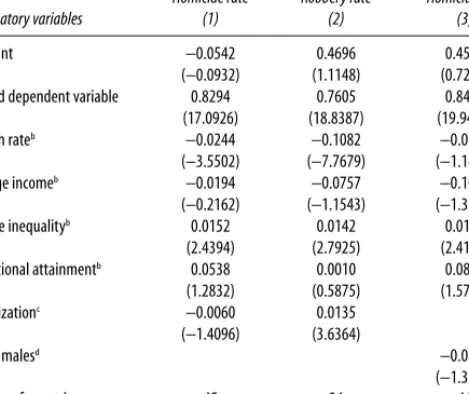
B A S I C E C O N O M I C D E T E R M I N A N T S. Table 2 presents the results on the basic economic model for homicide and robbery rates. To check the robustness of the results, we use two alternative sources for homicide sta-tistics, namely, the United Nations (UN) world crime surveys and the World Health Organization (WHO) mortality statistics. First, note that the Sargan and serial-correlation specification tests are supportive of the GMM system estimator and its assumptions. This is the case not only for the three regressions reported in table 2 but also for all results based on this GMM system methodology (tables 3–6). The homicide and robbery regressions of the basic economic model indicate that the GDP growth rate, the degree of income inequality as measured by the Gini index, and the respective lagged crime rates are significant and robust determinants of national crime rates.
The coefficients on per capita GNP change sign and significance in each of the three regressions, while educational attainment is not statistically significant in any of them. Thus the level of economic development, as measured by these two variables, does not appear to have an effect on the incidence of violent crimes. The fact that per capita income does not have a clear effect on violent crime rates when income inequality is held con-stant can be interpreted as evidence that the levelof poverty does not induce criminal behavior. However, when we combine the crime-inducing impact of higher inequality with that of lower GDP growth, we can con-clude that the rateof poverty alleviation is a significant determinant of violent crime rates. The lack of significance of educational attainment in T A B L E 2 . Basic Economic Modela
Homicide rate Homicide rate Robbery rate (WHO data) (UN data) (UN data)
Explanatory variables (1) (2) (3)
Constant 0.8171 −0.3886 −0.4965
(12.13937) (−0.52762) (−0.8658)
Lagged dependent variable 0.8376 0.7263 0.7673
(12.1394) (12.2731) (23.4132) Growth rateb −0.0115 −0.0239 −0.1468 (−6.4619) (−2.9616) (−10.3282) Average incomec −0.0805 0.0090 0.1280 (−7.4297) (0.0783) (2.4637) Income inequalityd 0.0035 0.0146 0.0258 (5.9282) (2.2671) (3.7501) Educational attainmente −0.0013 0.0354 −0.0016 (−0.2347) (0.6907) (−1.3333) Number of countries 48 45 34 Number of observations 193 136 102
Specification tests (p value)
Sargan test 0.532 0.226 0.446
Serial correlation
First order 0.008 0.068 0.043
Second order 0.592 0.284 0.803
Source: Authors’calculations based on WHO mortality statistics;UN world crime surveys (various issues) for crime data.For other vari-ables, see the sources listed in the appendix.
a. Dependent variables are expressed in logs.Estimation technique is the generalized method of moments (GMM) system estimator; tstatistics are in parentheses. For details of definitions and sources of variables, see appendix.
b. Percent annual change in real GDP. c. Log of per capita GNP in dollars. d. Gini coefficient.
our violent crime regressions confirms the education puzzle first noticed by Ehrlich.79
The past incidence of crime is another significant determinant of violent crime rates, which represents evidence in favor of the existence of crime waves. Past crime can breed future crime through a couple of channels. First, the costs of performing criminal activities decline over time given that, as in any other activity, criminals learn by doing.80The moral loss from breaking the law may also be reduced by social interactions with other criminals, and job opportunities in the legal labor market are likely to be reduced by the stigma associated with past criminal records.81A second channel that explains the observed criminal inertia is that the police and judicial systems fail to respond to jumps in the incidence of criminal behavior, which encourages further crime by reducing the perceived prob-abilities of apprehension and conviction of criminals.82
Criminal inertia implies that the long-run effect of a sustained change in one of the variables that affect crime rates is a multiple of its short-run effect (which is given by the corresponding coefficient as reported in the tables). In the case of homicides, long-run effects are 3.7 times larger than the short-run effects; and in the case of robberies, 4.3 times. In the case of transitory shocks, criminal inertia implies that the effect of a shock lasts longer than the shock itself. According to the estimated per-sistence coefficients, the half-life of a one-period shock to the homicide rate is 2.2 periods, and the corresponding half-life for the robbery rate is 2.6 periods.
The negative impact of GDP growth on violent crime rates indicates that the incidence of crime is countercyclical and that stagnant economic activity induces heightened criminal activity. By increasing the availabil-ity of job opportunities and raising wages in the legal vis-à-vis the crimi-nal labor market, economic growth has a crime-reducing effect. The fact that this result holds not only for robbery but also for homicide rates may indicate that an important fraction of homicides results from economically motivated crimes that become violent.83
79. Ehrlich (1975b).
80. See Glaeser, Sacerdote, and Scheinkman (1996). 81. See Leung (1995).
82. See Sah (1991); Posada (1994).
83. An alternative explanation is that economic conditions may have a cognitive impact on individuals by affecting their moral values or tolerance for crime.
The estimated coefficients for the growth rate are not only statistically significant, but they are also economically important in magnitude. For homicides, the estimated growth coefficient implies that a one percentage point increase in the GDP growth rate is associated with a 2.4 percent decline in the homicide rate in the short run. In the case of robberies, a sim-ilar increase in the GDP growth rate leads to a short-run fall of 13.7 percent in the robbery rate, that is, more than five times higher than for the homi-cide rate. Thus economic activity, using the GDP growth rate as a proxy, has a larger impact on typically economic crimes, such as robberies, than on more violent crimes, such as homicides.
The positive effect of income inequality on the homicide and robbery rates can be interpreted as the impact of the difference between the returns on crime (as measured by the income of the victims) and its opportunity cost (as measured by the legal income of the most disfavored citizens). This argument, initially made by Ehrlich, is based on the assumption that crime victims are relatively richer than their aggressors; it may not apply to crimes where victims and perpetrators share common social and economic characteristics.84An alternative interpretation of the positive link between inequality and crime is that in countries with higher income inequality, individuals have lower expectations of improving their social and eco-nomic status through legal ecoeco-nomic activities, which would decrease the opportunity cost of participating in illegal endeavors. Pessimistic percep-tions of economic improvement through legal activities could also lead to a lessening of the moral dilemma associated with breaking the law.
Other factors may explain the positive link between inequality and crime. Bourguignon argues that “the significance of inequality as a deter-minant of crime in a cross-section of countries may be due to unobserved factors affecting simultaneously inequality and crime rather than to some causal relationship between these two variables.”85One such factor that could lead to a spurious correlation between income inequality and crime rates is the limited amount and unequal distribution of crime prevention efforts that could be present in more unequal countries. We explore this possibility below when we include proxies of deterrence in our empirical model. Other factors that could affect both income inequality and crime are the existence of educational inequality and the degree of income and
84. Ehrlich (1973, pp. 538–40). 85. Bourguignon (1998, p. 2).