University of New Orleans University of New Orleans
ScholarWorks@UNO
ScholarWorks@UNO
Senior Honors Theses Undergraduate Showcase
Spring 2019
Identification of RNA Binding Proteins and RNA Binding Residues
Identification of RNA Binding Proteins and RNA Binding Residues
Using Effective Machine Learning Techniques
Using Effective Machine Learning Techniques
Reecha Khanal
University of New Orleans
Follow this and additional works at: https://scholarworks.uno.edu/honors_theses Part of the Computer Sciences Commons
Recommended Citation Recommended Citation
Khanal, Reecha, "Identification of RNA Binding Proteins and RNA Binding Residues Using Effective Machine Learning Techniques" (2019). Senior Honors Theses. 128.
https://scholarworks.uno.edu/honors_theses/128
This Honors Thesis-Restricted is protected by copyright and/or related rights. It has been brought to you by ScholarWorks@UNO with permission from the rights-holder(s). You are free to use this Honors Thesis-Restricted in any way that is permitted by the copyright and related rights legislation that applies to your use. For other uses you need to obtain permission from the rights-holder(s) directly, unless additional rights are indicated by a Creative Commons license in the record and/or on the work itself.
This Honors Thesis-Restricted has been accepted for inclusion in Senior Honors Theses by an authorized administrator of ScholarWorks@UNO. For more information, please contact [email protected].
Identification of RNA Binding Proteins and RNA Binding Residues Using Effective Machine Learning Techniques
An Honors Thesis
Presented to
the Department of Computer Science
of the University of New Orleans
In Partial Fulfillment
of the Requirements for the Degree of
Bachelor of Science, with University High Honors
and Honors in Computer Science
by
Reecha Khanal
ii
Acknowledgements
Initially, I would like to thank Dr. Md Tamjidul Hoque and Mr. Avdesh Mishra for their continuous guidance and mentorship through my thesis and research works. I am also grateful to the Department of Computer Science at the University of New Orleans for all the resources that had been provided to me, without which this research work would not have been possible.
Furthermore, I highly appreciate the support from Tolmas Scholars program without which I would not be able to be involved in on-campus research activities. I would also like to thank Dr. Christopher M. Summa for being the second reader for my thesis and Ms. Erin Spence Sutherland for her continuous guidance and support through the entire tenure of my undergraduate degree.
iii
Table of Contents
List of Tables………...…………. vi
List of Figures………...……… vii
Abstract……….….……….. viii
1.0 Introduction……….………... 1
1.1 Thesis Overview………..…... 1
1.2 Contribution of the Thesis………... 1
1.3 Technical results of the Thesis………..…... 2
1.4 Thesis Organization………... 3
1.5 Related Publications………... 3
2.0 Accurate Identification of RNA-binding Proteins Using Machine Learning Techniques……. 4
2.1 Introduction……….………... 4
2.2 Methods………...……... 8
2.2.1 Dataset……….…………..………..………... 9
2.2.1.1 Benchmark Dataset ………...……….. 9
2.2.1.2 Independent Test Dataset ……….... 9
iv
2.2.2.1 Features Extracted from Physicochemical Properties ... 11
2.2.2.2 Features Extracted from Evolutionary Information.………..…… 18
2.2.2.3 Features Extracted to account for Intrinsically Disordered Regions……….. 18
2.2.3 Performance Evaluation……….…... 21
2.2.4 Feature Selection ……….. 23
2.2.4.1 Feature Selection using IFS………... 23
2.2.4.2 Feature Selection using GA……….. 24
2.2.5 AIRBP Framework ….………... 25
2.3 Results………...…….. 28
2.3.1 Feature Selection ……….. 29
2.3.2 Selection of classifiers for stacking………. 30
2.3.3 Performance Comparison on the benchmark dataset……….………... 32
2.3.4 Performance Comparison using the independent test dataset…...……... 33
2.4 Conclusions……….…….………... 35
3.0 Prediction of RNA Binding residue using Advanced Machine Learning Techniques ……… 37
3.1 Introduction ……… 37
v
3.2.1 Datasets……….. 40
3.2.2 Feature Extraction ………. 41
3.2.3 Feature Selection using Genetic Algorithm ……….. 46
3.2.4 Window Selection ……….. 48
3.2.5 Performance Evaluation ………. 49
3.2.6 Framework of our RBP residue Predictor ……… 50
3.3 Results ……….... 53
3.3.1 Selection of Classifiers for Stacking……… 53
3.3.2 Future Works ………... 54
3.4 Conclusions ……… 55
4.0 Conclusions and Recommendations……….………... 56
4.1 Summary………... 56
4.2 Future Scope……….…………... 57
vi List of Tables
Table 1. RCEM table used in the proposed experiment………. 20 Table 2. Name and definition of the evaluation metric………... 22 Table 3 Comparison of Incremental Feature Selection and Feature Selection using Genetic Algorithm for AIRBP ………... 29
Table 4. Comparisons of various base learners on the benchmark dataset using jackknife cross-validation for AIRBP ………..…….. 30
Table 5. Comparisons of stacked models with different set of base-classifiers through jackknife validation ………... 31
Table 6. Comparisons of AIRBP with the state-of-the-art method RBPPred on independent training dataset ………...……… 32
Table 7 Comparisons of AIRBP with the state-of-the-art method RBPPred on independent test dataset, ……….. 34
Table 8. Performance of various window sizes on the benchmark dataset using the XGB for RNA-binding residue prediction………... 48 Table 9. Comparisons of various base learners on the benchmark dataset using jackknife cross-validation for RNA Binding Residue Predictor ………...…... 53
vii List of Figures
Figure 1. Working of C-T-D ……….……… 13
Figure 2. Working of CT ……….. 15
viii
Abstract:
Identification and annotation of RNA Binding Proteins (RBPs) and RNA Binding residues from sequence information alone is one of the most challenging problems in computational biology. RBPs play crucial roles in several fundamental biological functions including transcriptional regulation of RNAs and RNA metabolism splicing. Existing experimental techniques are time-consuming and costly. Thus, efficient computational identification of RBPs directly from the sequence can be useful to annotate RBP and assist the experimental design. Here, we introduce AIRBP, a computational sequence-based method, which utilizes features extracted from evolutionary information, physiochemical properties, and disordered properties to train a machine learning method designed using stacking, an advanced machine learning technique, for effective prediction of RBPs. Furthermore, it makes use of efficient machine learning algorithms like Support Vector Machine, Logistic Regression, K-Nearest Neighbor and XGBoost (Extreme Gradient Boosting Algorithm). In this research work, we also propose another predictor for efficient annotation of RBP residues. This RBP residue predictor also uses stacking and evolutionary algorithms for efficient annotation of RBPs and RNA Binding residue. The RNA-binding residue predictor also utilizes various evolutionary, physicochemical and disordered properties to train a robust model. This thesis presents a possible solution to the RBP and RNA binding residue prediction problem through two independent predictors, both of which outperform existing state-of-the-art approaches.
1
Introduction:
1.1Thesis Overview:
Today, there has been a lot of development in genomics and hence there is an increased number of proteomic data available in different online databases. Experimental methods alone are time consuming and costly. So, bioinformatics offers a faster, cheaper way to mine, evaluate and interpreted such biological data. Today, bioinformatics has become essential in dealing with biological data because of its efficiency and success in various research works. The development of computational tools for analysis and interpretation of such data through bioinformatics involves few steps: i) Data mining, collection, and preparation of data, ii) Computing to extract useful information or characteristics, can also be thought of as features, from the data, iii) Apply various Machine Learning Algorithms to develop a robust classifier that uses the features extracted in the previous step, and iv) Analyze, compare and evaluate obtained results from the classifiers. These three steps have been utilized in this thesis to develop predictors for annotation of RNA Binding Proteins and RNA Binding residues.
1.2Contribution of the Thesis:
This thesis aims to solve one of the most important problems in bioinformatics by providing predictors for efficient annotation of both RNA Binding Proteins and RNA Binding Residues using the sequence information of the protein alone. The predictors developed could also be used to assist experimental inquiries and can also be used as a stepping stone for other prediction methods.
2
1.3 Technical results of the Thesis:
Technical results of this thesis can be divided into two parts: i) A predictor for prediction of RNA Binding Proteins, named AIRBP, and ii) A predictor for prediction of RNA Binding Residues. The two results are described below:
- A predictor for prediction of RNA Binding Proteins (AIRBP)
Here, we present a predictor for effective annotation of RNA Binding Proteins called AIRBP. AIRBP is a stacking based predictor that utilizes a pool of base learners like Extremely Randomized Trees, Random Forest, Logistic Regression, K-Nearest Neighbor and XGBoost (Extreme Gradient Boosting Algorithm). This predictor is fast and efficient and outperforms all other existing predictors for RNA Binding Proteins. It also provides a balanced performance on all the performance metrics and provides biologically relevant prediction of RNA Binding Proteins.
- A predictor for prediction of RNA Binding Residues
In addition to the RNA Binding Protein predictor, this research also presents a predictor for RNA Binding Residues or sites present in the RNA Binding Proteins. This predictor uses software like DisPredict, SPIDER, and SCRATCH to obtain various evolutionary, physicochemical and disordered properties of RNA Binding Proteins. This work, similar to AIRBP, which uses advanced machine learning frameworks like Stacking and Genetic Algorithms.The results from our study show that the generated predictor is well balanced on all the performance metrics and provides biologically relevant prediction of RNA Binding Residues.
3
1.4 Thesis Organization:
The primary aim of the thesis is to develop a computational approach for the prediction of RNA-binding proteins using only sequence information. The rest of the thesis is organized as follows: Chapter 2 discusses the design and development of RBP predictor. The details on datasets, feature extraction, and performance evaluation are provided in Chapter 2. Chapter 3 discusses the design and development of RBP residues predictor. The details on datasets, feature extraction, and performance evaluation are provided in Chapter 3. Finally, Chapter 4, concludes this thesis and states the major contributions and provides future directions and possibilities for further research to make the tools as accurate as possible.
1.5 Related Publications:
Below listed are research works that have provided noteworthy results in the world of RBP prediction.
1. Zhang, X. and Liu, S. RBPPred: predicting RNA-binding proteins from sequence using SVM. Bioinformatics 2017;33(6):854-862.
2. Avdesh Mishra, Reecha Khanal§, Md Tamjidul Hoque*, “Accurate Identification of RNA-binding Proteins (AIRBP) Using Machine Learning Techniques”, The 7th Annual Conference on Computational Biology and Bioinformatics, Louisiana, USA, 2019 [Poster].
3. Su, H., et al. (2019) Improving the prediction of protein–nucleic acids binding residues via multiple sequence profiles and the consensus of complementary methods, Bioinformatics, 35, 930-936.
Part of this thesis has also been presented as posters and oral presentation in the 6th and 7th Annual
4 Chapter 2
AIRBP: Accurate Identification of RNA-Binding Proteins Using Machine Learning Techniques
2.1 Introduction
RNA Binding Proteins (RBPs) are proteins that bind to ribonucleic acid (RNA) molecules and form dynamic units, called ribonucleoprotein (RNP) complexes. These RBPs along with the RNP complexes play a crucial role starting from the biogenesis process of RNA to its degradation (Beckmann, et al., 2015). Additionally, they contribute to several important biological functions that include RNA transport, cellular localization, gene expression, expression of histone genes, post-transcriptional gene regulation, and regulation of translation and transcription control (Glisovic, et al., 2008). As an illustration, the newly formed messenger RNA, that carries necessary genetic information from DNA to ribosomes, associates with various RNA binding proteins (RBP) to form messenger ribonucleoprotein (mRNP) complexes (Baltz, et al., 2012). These mRNP complexes govern major elements of metabolism and functions of mRNA. Similarly, the microRNPs (miRNPs), formed through association of the RBPs with microRNAs (miRNAs) controls the translation and stability of RNA itself (Wurth, 2012). The identification of RBPs along with their mRNA targets is shown useful in cancer therapy (Wurth, 2012). There are numerous other diseases that have been linked to defective RBP expression and functions, including neuropathies, muscular atrophies, and metabolic disorders (Castello, et al., 2012), highlighting the urgency of identifying possible RBPs.
As of today, numerous studies have been performed and various experimental and computational methods have been developed to identify and expand our knowledge of RBPs. The initial steps
5
towards identification and study of RBPs and RNP complexes date back to almost half a century ago where experimental methods such as purification of mRNPs from in vitro UV-irradiated polysomal fractions (Greenberg, 1979), from UV-irradiated intact cells (Wagenmakers, et al., 1980) and from untreated cells (Lindberg and Sundquist, 1974) revealed the association of a specific set of proteins with mRNA (Baltz, et al., 2012). Recently, cutting-edge experimental approaches are developed to recognize numerous RBPs, which include identification of 860 RBPs in human HeLa cells (Castello, et al., 2012) using UV crosslinking methods, 797 RBPs in human embryonic kidney cell line (Baltz, et al., 2012) using photoreactive nucleotide-enhanced UV crosslinking and oligo(dT) purification approach, 555 mRNA-binding proteins from mouse embryonic stem cells (Kwon, et al., 2013) using UV crosslinking, oligo(dT) and Mass Spectrometry and 120 RBPs from S. cerevisiae cells (Mitchell, et al., 2013) using UV crosslinking and purification methods. These experiments for identifying and analyzing of RBPs, have broadened our understanding of RBPs to a certain extent. Despite the great efforts and achievements, these experiments are expensive, time-consuming and labor-intensive (Si, et al., 2015). Moreover, the tremendous progress in genome sequencing has resulted in an unprecedented amount of genetic information and provided a plethora of protein sequences (Wu, et al., 2006), which outpace the tasks of annotating them and elucidating their functions. Thus, it becomes urgent to have faster and more accurate computational approaches to build an RBP repository and RNA-RBP interaction network maps.
In the recent past, several attempts have been made in identifying RNA-binding proteins and many effective computational prediction methods have been developed, which can be divided into two broad categories: i) templated based; and ii) machine learning based. Template based methods extract significant structural or sequence similarity between the query and a template known to
6
bind RNA, to assess the RNA-binding preference of the target sequence (Yang, et al., 2012; Zhao, et al., 2011; Zhao, et al., 2011). Unlike template based methods, in machine learning methods the predictive model is created to make the prediction by finding a pattern in the input feature space (Kumar, et al., 2011; Paz, et al., 2016; Shazman and Mandel-Gutfreund, 2008). The machine learning approaches vary in the features employed and the classification algorithm used.
Zhao et al. proposed two template based approaches for predicting RBPs, of which, SPOT-stru (Zhao, et al., 2011) is a structure based approach and SPOT-seq (Zhao, et al., 2011) is a sequence based approach. In SPOT-stru, the relative structural similarity in the form of Z-score and a statistical energy function DFIRE is used to predict RBPs. The results indicate that SPOT-seq achieved the Matthew’s Correlational Coefficient (MCC), which is a performance evaluation parameter used in machine learning as a measure of the quality of binary classifications, of 0.57 on the benchmark data of 212 RNA-binding domains and 6761 non-RNA binding domains. On the other hand, in SPOT-seq the fold recognition between the target sequence and template structures using the defined sequence-structure matching score is used to predict RBPs. As shown, SPOT-seq achieved the MCC of 0.62 on the benchmark data of 215 RBP chains and 5765 non-binding protein chains.
The machine learning based approach for the prediction of RNA-binding proteins involves two important steps: i) extraction of relevant features, and ii) selection of an appropriate classification algorithm. Furthermore, depending on the feature extraction mechanism, the existing predictive method can be segmented into two different categories: i) extraction of relevant features from the structure of protein (Paz, et al., 2016; Shazman and Mandel-Gutfreund, 2008); and ii) extraction of relevant features from protein sequence (Kumar, et al., 2011; Ma, et al., 2015; Ma, et al., 2015; Zhang and Liu, 2017). BindUp (Paz, et al., 2016) available as a web server, is one of the recent
7
structure-based methods that extracts electrostatic features and other properties from the structure of the protein and uses SVM classifier for RBPs prediction. As reported, BindUp attains sensitivity, a measure of proportion of actual positives that are correctly identified by a machine learning model, of 0.71 and specificity, a measure of proportion of actual negatives that are correctly identified as such by a machine learning model, of 0.96 on an independent test set of 323 structures of RNA binding proteins and a control set of an equal number extracted from Protein Data Bank (PDB). Towards sequence-based approaches, Ma et al. (Ma, et al., 2015; Ma, et al., 2015) recently proposed two different methods, which differ in the features used to train the random forest model for predicting. In (Ma, et al., 2015), the authors incorporated features of evolutionary information combined with physicochemical features (EIPP) and amino acid composition feature to develop the random forest predictor. Besides, in (Ma, et al., 2015), the authors employed features such as a conjoint triad, binding propensity, non-binding propensity, and EIPP to establish random forest based predictor with the minimum redundancy maximum relevance (mRMR) method, followed by incremental feature selection (IFS). As reported, their method achieved an accuracy of 0.8662 and MCC of 0.737. Most recently, Zhang and Liu (Zhang and Liu, 2017) proposed a new sequence-based approach, namely RBPPred which, integrates the physiochemical properties with the evolutionary information extracted from Position Specific Scoring Matrix (PSSM) profile and utilizes SVM to predict RBPs. As shown, RBPPred correctly predicted 83% of 2780 RBPs and 96% of 7093 non-RBPs with MCC of 0.808 using the 10-fold cross-validation (CV) approach. Despite significant progress, most of the approaches for RBPs prediction developed in the past are limited in explaining how protein-RNA interactions occur. Thus, it is essential to identify new features, effective encoding techniques and advanced machine
8
learning techniques that can help further improve the accuracy of RBPs predictors and ultimately improve our understanding of RNA-protein interactions and their functions.
In this work, we explore different sequence-based features, encoding techniques, and machine learning approaches, to further improve the prediction accuracy of RNA-binding proteins and our understanding of the binding mechanism of RNA-protein interactions. We propose a method, AIRBP, which utilizes features: Evolutionary Information (EI), Physiochemical Properties (PP), and Disordered Properties (DP). It uses four different types of feature encoding technique: Composition, Transition and Distribution (C-T-D) (Zhang and Liu, 2017), Conjoint Triad (CT) (Wang, et al., 2013; Zhang and Liu, 2017), PSSM Distance Transformation (PSSM-DT) (Mishra, et al., 2018; Xu, et al., 2015) and Residue-wise Contact Energy Matrix Transformation (RCEM-T) (Mishra, et al., 2018). Furthermore, AIRBP utilizes an ensemble machine learning framework, known as stacking (Wolpert, 1992) to predict RBPs from protein sequence only. AIRBP offers a significant improvement in the prediction of RBPs based on the benchmark and independent test datasets when compared to the existing start-of-the-art predictors. We believe that the superior performance of AIRBP will motivate the researchers to use it to identify RNA-binding proteins from sequence information. Moreover, the proposed stacking based machine learning technique, encoding techniques and features discussed in this work could be applied to tackle other relevant biological problems.
2.2 Methods
In this section, we describe the approach for benchmark and independent test data preparation, feature extraction and encoding, performance evaluation metrics and finally, the approach we took to establish the machine learning framework for RBPs prediction.
9
2.2.1Dataset
2.2.1.1 Benchmark Dataset
For this work, we collected the updated version of the benchmark dataset from (Liu; Zhang and Liu, 2017). The updated benchmark dataset was created by the authors (Zhang and Liu, 2017) from the original benchmark dataset by removing 16 proteins that had RNAs in their crystal structure from the negative set. Therefore, the updated benchmark dataset we collected consist of 7077 non-RBPs (16 proteins removed from the original benchmark dataset which contained 7093 non-non-RBPs) and 2780 RBPs (same as the original benchmark dataset). Next, we found that 13 out of 2780 and 90 out of 7077 protein sequences in RBPs and non-RBPs set respectively, contained non-standard amino acids (amino acids other than the 20 standard amino acids). These sequences containing non-standard amino acids were removed from further consideration as the physiochemical properties of non-standard amino acids could not be obtained. Finally, the benchmark dataset which contains 2767 RBPs and 6987 non-RBPs was obtained and used for validation and model creation of AIRBP.
2.2.1.2 Independent Test Set
To test the performance of AIRBP, we collected the updated independent test dataset from (Liu; Zhang and Liu, 2017). This dataset consists of independent test sets for 3 species, human, Saccharomyces cerevisiae (S. cerevisiae) and Arabidopsis thaliana (A. thaliana). The updated independent test set was created by the authors (Zhang and Liu, 2017) from the original independent test set by removing 9 proteins from the human set and 7 proteins from S. cerevisiae set that had RNAs in their crystal structure from the negative set, respectively. The updated independent test sets contained a total of 967 RBPs and 588 non-RBPs for human, 354 RBPs and
10
135 non-RBPs for S. cerevisiae and 456 RBPs and 37 non-RBPs for A. thaliana. Next, we removed the protein sequences containing non-standard amino acid from each of these independent set and finally obtained 967 RBPs and 584 non-RBPs for human, 354 RBPs and 134 non-RBPs for S. cerevisiae and 456 RBPs and 36 non-RBPs for A. thaliana.
2.2.2Feature Extraction
To create an effective RBPs predictor from sequence alone, the feature vector for each protein sequence was derived from the PSSM profile, Physiochemical Properties (PP), Residue-wise Contact Energy Matrix (RCEM) and Molecular Recognition Features (MoRFs). Total of 10 different properties was encoded with a vector of 2603 dimension to represent a protein sequence as shown in Supplementary Fig. 1S. Out of 10, five distinct properties hydrophobicity, polarity, normalized van der Waals volume, polarizability and predicted secondary structure were each encoded via 21 dimension vector utilizing C-T-D encoding technique (Dubchak, et al., 1995; Zhang and Liu, 2017). Moreover, the remaining five properties solvent accessibility, charge and polarity of the side chain, MoRFs, RCEM, and PSSM profile were encoded via 13, 64, 1, 20 and 2400 dimensional vectors, respectively. Here, the properties solvent accessibility, charge, and polarity of the side chain, RCEM, and PSSM profile were encoded utilizing C-T-D, CT (Wang, et al., 2013; Zhang and Liu, 2017), RCEM transformation (Mishra, et al., 2018) and PSSM-DT transformation techniques (Mishra, et al., 2018; Xu, et al., 2015). Each of the 10 properties along with their encoding mechanism is described next in detail.
11
2.2.2.1 Features Extracted from Physicochemical Properties
In this section we describe various feature extraction techniques, we utilized to obtain a fixed dimensional feature vector from the physicochemical properties which include hydrophobicity, polarity, normalized van der Waals volume, polarizability, predicted secondary structure, solvent accessibility and charge and polarity of the side chain to encode protein sequence.
2.2.2.1.1 Composition, Transition and Distribution (C-T-D) Transformation Features
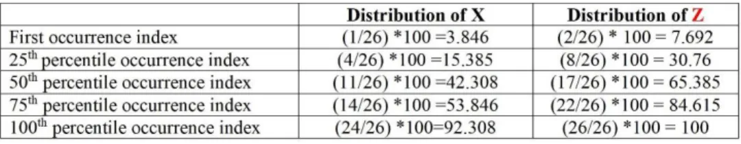
The aim of C-T-D transformation method is to describe the distribution patterns of amino acid properties. This method to compute distribution patterns of amino acid properties were first suggested by (Dubchak, et al., 1995) for protein fold class prediction. In our implementation, we used C-T-D transformation to encode the properties including hydrophobicity, polarity, normalized van der Waals volume, polarizability, predicted secondary structure and solvent accessibility. As the name suggests, this transformation technique focuses on three different components: composition of a particular amino acid in the sequence, transition of one amino acid to other as we go linearly through the sequence, and distribution referring to how one amino acid group is distributed throughout the protein sequence (Han, et al., 2004; Zhang and Liu, 2017). To create a consistent number of features for proteins with different sequence length, 20 standard amino acids are divided into 3 groups (Dubchak, et al., 1999) based on their hydrophobicity, normalized van der Waals volume, polarity, and polarizability. Fig 1. provides an illustration of C-T-D transformation technique while, the 20 standard amino acids are divided into 2 groups which, generates a feature vector of 13 dimensions. Following the transformation technique shown in Fig.1 with an exception that the 20 standard amino acids are divided into 3 groups, we obtain a
12
feature vector of 21 dimensions for the physiochemical properties such as hydrophobicity, normalized van der Waals volume, polarity, and polarizability.
Furthermore, to encode the predicted secondary structure and solvent accessibility as features, we first used the SSpro and ACCpro program (Magnan and Baldi, 2014) to predict secondary structure in the form of ‘H’ (helix), ‘E’ (strand) and ‘C’ (other than helix and strand) and solvent accessibility in the form of ‘e’ (exposed residues) and ‘-’ (buried residues), respectively. The choice of SSpro and ACCpro was made to extract predicted secondary structure and solvent accessibility because of its superior performance and remarkable speed. As reported SSpro and ACCpro (Magnan and Baldi, 2014) achieved an accuracy of 92.9% and 90% for secondary structure prediction and relative solvent accessibility prediction, respectively. Using the transformation technique described above, we obtained feature vectors of 21 and 13 dimensions for predicted secondary structure and solvent accessibility, respectively.
13
Fig. 1. Illustration of C-T-D transformation technique, while the 20 standard amino acids are divided into 2 groups (e.g. X and Z). First, the group index (X or Z) of every amino acid in the protein sequence is extracted and consequently, a vector of 13 dimensions is obtained through composition, transition, and distribution.
14
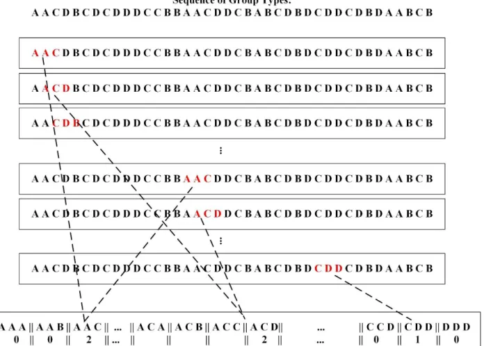
The CT transformation technique was first proposed by Shen et al. for protein-protein interaction prediction (Shen, et al., 2007) and has been successfully applied for protein-RNA interaction prediction in the past (Wang, et al., 2013; Zhang and Liu, 2017). In our implementation, we adopted the CT transformation technique to encode the protein sequence based on the charge and polarity of the side chain of the amino acids in a protein. First, the 20 standard amino acids are divided into 4 groups: i) acidic (contain residues D and E); ii) basic (contain residues H, R and K); iii) polar (contain residues C, G, N, Q, S, T, and Y); and iv) non-polar (contain residues A, F, I, L, M, P, V, and W) according to their charge and polarity of the side chain. Then, the protein sequence is converted into a sequence of group types where each element in the sequence represents a group type of the corresponding amino acid in the protein sequence. Next, a triad of three contiguous amino acids is considered as a single unit. Accordingly, all the triads can be classified into 4 × 4 × 4 = 64 classes. Finally, a sliding window of a triad is passed through a sequence of group types and the frequency of occurrences of each type of triad is counted. Through this process, we obtain a feature vector of 64 dimensions for charge and polarity of side chains of amino acids in a protein. Supplementary Fig. 2 provides an illustration of CT transformation technique we used to extract features from protein sequence based on charge and polarity of side chains.
15
Fig. 2. Illustration of Conjoint Triad transformation technique while, the 20 standard amino acids are divided into 4 groups (Group A, B, C and D representing acidic, basic, polar and non-polar, respectively).
16
2.2.2.2 Features Extracted from Evolutionary Information
In this section, we describe various feature extraction techniques utilized to obtain a fixed dimensional feature vector from the evolutionary information, called the PSSM profile, to encode the protein sequence.
Evolutionary information is one of the most important information useful for solving various biological problems and has been widely used in many research work (Iqbal, et al., 2015; Kumar, et al., 2007; Kumar, et al., 2008; Kumar, et al., 2011; Mishra, et al., 2018; Zhang and Liu, 2017). In this work, the evolutionary information in the form of PSSM profile is directly obtained from the protein sequence and later transformed into a fixed dimensional vector. PSSM captures the conservation pattern in multiple alignments and preserves it as a matrix for each position in the alignment. High score in the PSSM matrix indicates more conserved positions and the lower score indicates less conserved positions (Mishra, et al., 2018). For this study, we generated the PSSM profile for every protein sequence by executing three iterations of PSI-BLAST against NCBI’s non-redundant database (Altschul, et al., 1990). The evolutionary information in PSSM profile is represented as a matrix of L*20 dimensions, where L is the length of the protein sequence. A particular element Mi,j of the PSSM matrix represents the occurrence probability of the amino acid
i at position j of a protein sequence.
2.2.2.2.1 PSSM-Distance Transformation (PSSM-DT) Features
We use two types of distance transformation techniques (Mishra, et al., 2018; Xu, et al., 2015): i) the PSSM distance transformation for same pairs of amino acids (PSSM-SDT); and ii) the PSSM distance transformation for different pairs of amino acids (DDT), together known as PSSM-DT to extract fixed dimensional feature vectors of size 100 and 1900, respectively.
17
Utilizing PSSM-SDT, we compute the occurrence probabilities for the pairs of the same amino acids separated by a distance D along the sequence, which can be represented as:
𝑃𝑆𝑆𝑀-𝑆𝐷𝑇(𝑗, 𝐷) = ∑ 𝑀𝑖,𝑗∗ 𝑀𝑖+𝐷,𝑗/(𝐿 − 𝐷) 𝐿−𝐷
𝑖=1
(1)
where, j represents one type of the amino acid, L represents the length of the sequence, Mi,j represents the PSSM score of amino acid j at position i, and Mi+D,jrepresents the PSSM score of amino acid j at position i+D. Through this approach, 20 K number of features were generated where K is the maximum range of D (D = 1,2, …, K).
Likewise, utilizing PSSM-DDT, we compute the occurrence probabilities for pairs of different amino acids separated by a distance D along the sequence, which can be represented as:
𝑃𝑆𝑆𝑀-𝐷𝐷𝑇(𝑖1, 𝑖2, 𝐷) = ∑ 𝑀𝑗,𝑖1 ∗ 𝑀𝑗+𝐷,𝑖2 /(𝐿 − 𝐷) 𝐿−𝐷
𝑗=1
(2)
where, 𝑖1 and 𝑖2 represent two different types of amino acids. The total number of features obtained by PSSM-DDT is 380 K. Here, we consider K = 5, therefore a total of 100 features was obtained by PSSM-SDT and a total of 1900 features was obtained by PSSM-DDT transformation techniques.
2.2.2.2.2 Evolutionary Distance Transformation (EDT) Features
Unlike PSSM-DT, the EDT approximately measures the non-co-occurrence probability of two amino acids separated by a certain distance d in a protein sequence from the PSSM profile (Mishra, et al., 2018; Zhang, et al., 2014). The EDT is calculated from the PSSM profile as:
18 𝑓(𝑅𝑥, 𝑅𝑦) = ∑ 1 𝐿 − 𝑑 ∑(𝑀𝑖,𝑥− 𝑀𝑖+𝑑,𝑦) 2 𝐿−𝑑 𝑖=1 𝐷 𝑑=1 (3)
where, d is the distance separating two amino acids, D is the maximum value of d, 𝑀𝑖,𝑥and 𝑀𝑖+𝑑,𝑦 are the elements in the PSSM profile, and 𝑅𝑥 and 𝑅𝑦 represent any of the 20 standard amino acids in the protein sequence. Here, the value of D = Lmin-1 where, Lmin is the length of the shortest protein sequence in the benchmark dataset. Using EDT, we obtain a feature vector of dimension 400.
2.2.2.3 Features Extracted to Account for Intrinsically Disordered Regions
In this section we describe a feature extraction technique utilized to obtain a fixed dimensional feature vector from residue-wise contact energy matrix, to encode protein sequence.
RBPs are found to bind with RNA not only through classical structured
RNA-binding domains but also through intrinsically disordered regions (IDRs) (Calabretta and Richard, 2015). For example, approximately 20% of the identified mammalian RBPs (~170 proteins) were found to be disordered by over 80% (Järvelin, et al., 2016). The energy contribution of a large number of inter and intra-residual interactions in intrinsically disordered proteins (IDPs) cannot be approximated by the energy functions extracted from known structures (Hoque, et al., 2016; Iqbal, et al., 2015; Mishra and Hoque, 2017; Mishra, et al., 2016; Zhou and Skolnick, 2011) as IDPs lack a defined and ordered 3D structure (Babu, et al., 2011). Therefore, to inherently incorporate important information regarding the IDRs and amino acid interactions, we employed the predicted residue-wise contact energies (Dosztányi, et al., 2005) and molecular recognition features (MoRFs) (Sharma, et al., 2018), to encode the protein sequence.
19
2.2.2.3.1 Residue-Wise Contact Energy Matrix Transformation (RCEM-T) Features
We adopted the predicted residue-wise contact energy matrix (RCEM) derived in (Dosztányi, et al., 2005), by the least square fitting of 674 proteins primary sequence with the contact energies derived from the tertiary structure of 785 proteins. As shown in Table 1, the RCEM is a 20 × 20 dimensional matrix which contains residue-wise contact energy for 20 standard amino acids. For a protein sequence of length L, an L × 20 dimensional matrix M is obtained which holds 20 dimensional vector for each amino acid in a protein sequence. The resulting matrix M is then encoded into a feature vector of 20 dimensions by computing the column-wise sum as:
𝑓(𝐴𝑗) = ∑ 𝑚𝑖,𝑗 𝐿
𝑖=1
(𝑗 = 1,2, ⋯ , 20) (4)
where, mi,j is the element of matrix M, i is the amino acid index in a sequence and j represents 20 standard amino acid types. The final feature vector, 𝑅𝐶𝐸𝑀 − 𝑇 = [𝑣1, 𝑣2, ⋯ , 𝑣20] is obtained by dividing each element in RCEM-T by the sum of all the elements in the same vector. Considering Vs as the sum of all the elements in the RCEM-T vector, each element in the final
RCEM-T vector can be represented as:
𝑅𝐶𝐸𝑀𝑇(𝑣𝑖) = 𝑣𝑖
20
Table 1. RCEM table to obtain RCEM-T features
A C D E F G H I K L M N P Q R S T V W Y A -1.65 -2.83 1.16 1.8 -3.73 -0.41 1.9 -3.69 0.49 -3.01 -2.08 0.66 1.54 1.2 0.98 -0.08 0.46 -2.31 0.32 -4.62 C -2.83 -39.58 -0.82 -0.53 -3.07 -2.96 -4.98 0.34 -1.38 -2.15 1.43 -4.18 -2.13 -2.91 -0.41 -2.33 -1.84 -0.16 4.26 -4 .46 D 1.16 -0.82 0.84 1.97 -0.92 0.88 -1.07 0.68 -1.93 0.23 0.61 0.32 3.31 2.67 -2.02 0.91 -0.65 0.94 -0.71 0. 90 E 1.8 -0.53 1.97 1.45 0.94 1.31 0.61 1.3 -2.51 1.14 2.53 0.2 1.44 0.1 -3.13 0.81 1.54 0.12 -1.07 1. 29 F -3.73 -3.07 -0.92 0.94 -11.25 0.35 -3.57 -5.88 -0.82 -8.59 -5.34 0.73 0.32 0.77 -0.4 -2.22 0.11 -7.05 -7.09 -8 .80 G -0.41 -2.96 0.88 1.31 0.35 -0.2 1.09 -0.65 -0.16 -0.55 -0.52 -0.32 2.25 1.11 0.84 0.71 0.59 -0.38 1.69 -1 .90 H 1.9 -4.98 -1.07 0.61 -3.57 1.09 1.97 -0.71 2.89 -0.86 -0.75 1.84 0.35 2.64 2.05 0.82 -0.01 0.27 -7.58 -3 .20 I -3.69 0.34 0.68 1.3 -5.88 -0.65 -0.71 -6.74 -0.01 -9.01 -3.62 -0.07 0.12 -0.18 0.19 -0.15 0.63 -6.54 -3.78 -5 .26 K 0.49 -1.38 -1.93 -2.51 -0.82 -0.16 2.89 -0.01 1.24 0.49 1.61 1.12 0.51 0.43 2.34 0.19 -1.11 0.19 0.02 -1 .19 L -3.01 -2.15 0.23 1.14 -8.59 -0.55 -0.86 -9.01 0.49 -6.37 -2.88 0.97 1.81 -0.58 -0.6 -0.41 0.72 -5.43 -8.31 -4 .90 M -2.08 1.43 0.61 2.53 -5.34 -0.52 -0.75 -3.62 1.61 -2.88 -6.49 0.21 0.75 1.9 2.09 1.39 0.63 -2.59 -6.88 -9 .73 N 0.66 -4.18 0.32 0.2 0.73 -0.32 1.84 -0.07 1.12 0.97 0.21 0.61 1.15 1.28 1.08 0.29 0.46 0.93 -0.74 0. 93 P 1.54 -2.13 3.31 1.44 0.32 2.25 0.35 0.12 0.51 1.81 0.75 1.15 -0.42 2.97 1.06 1.12 1.65 0.38 -2.06 -2 .09 Q 1.2 -2.91 2.67 0.1 0.77 1.11 2.64 -0.18 0.43 -0.58 1.9 1.28 2.97 -1.54 0.91 0.85 -0.07 -1.91 -0.76 0. 01 R 0.98 -0.41 -2.02 -3.13 -0.4 0.84 2.05 0.19 2.34 -0.6 2.09 1.08 1.06 0.91 0.21 0.95 0.98 0.08 -5.89 0. 36 S -0.08 -2.33 0.91 0.81 -2.22 0.71 0.82 -0.15 0.19 -0.41 1.39 0.29 1.12 0.85 0.95 -0.48 -0.06 0.13 -3.03 -0 .82 T 0.46 -1.84 -0.65 1.54 0.11 0.59 -0.01 0.63 -1.11 0.72 0.63 0.46 1.65 -0.07 0.98 -0.06 -0.96 1.14 -0.65 -0 .37 V -2.31 -0.16 0.94 0.12 -7.05 -0.38 0.27 -6.54 0.19 -5.43 -2.59 0.93 0.38 -1.91 0.08 0.13 1.14 -4.82 -2.13 -3 .59 W 0.32 4.26 -0.71 -1.07 -7.09 1.69 -7.58 -3.78 0.02 -8.31 -6.88 -0.74 -2.06 -0.76 -5.89 -3.03 -0.65 -2.13 -1.73 -1 2.39 Y -4.62 -4.46 0.9 1.29 -8.8 -1.9 -3.2 -5.26 -1.19 -4.9 -9.73 0.93 -2.09 0.01 0.36 -0.82 -0.37 -3.59 -12.39 -2 .68
2.2.2.3.2 Molecular Recognition Features (MoRFs)
MoRFs, also sometimes known as molecular recognition elements (MoREs), are disordered regions in a protein those exhibit various molecular recognition and binding functions (Vacic, et al., 2007). Post-translational modifications (PTMs) can induce disorder to order transitions of IDPs upon binding with their binding partners which could be either RNA, DNA, proteins, lipids,
21
carbohydrates or other small molecules (Bah and Forman-Kay, 2016; Lina, et al., 2017). MoRFs play a vital role in various biological functions of IDPs located within long disordered protein sequences (Mohan, et al., 2006; Sharma, et al., 2018; Sharma, et al., 2018; Sharma, et al., 2018). Additionally, Mohan et al. suggest that functionally significant residual structures exist in MoRF regions prior to the actual binding (Mohan, et al., 2006). These residual structures could, therefore, be useful in the prediction of binding between proteins and RNA. Here, to capture functional properties of IDRs which may bind to RNAs, we employ a single predicted MoRFs score as a feature. To obtain a single predicted MoRFs score, first, the residue-wise predicted MoRFs scores are obtained from the OPAL program (Sharma, et al., 2018). Then, a single predicted MoRFs score is computed by taking a ratio of the sum of the residue-wise MoRFs score and the length of the protein sequence.
2.3 Performance Evaluation
To evaluate the performance of AIRBP, we adopted a widely used 10-fold cross-validation (CV) and the independent testing approach. In the process of 10-fold CV, the dataset is segmented into 10 parts, which are each of about same size. When one fold is kept aside for testing, the remaining 9 folds are used to train the classifier. This process of training and test is repeated until each fold has been kept aside once for testing and consequently, the test accuracies of each fold are combined to compute the average (Hastie, et al., 2009). Unlike a 10-fold CV, in independent testing, the classifier is trained with the benchmark dataset and consequently tested using the independent test dataset. While independent testing, it is ensured that none of the samples in the independent test set are present in the benchmark dataset. We used several performance evaluation metrics listed in
22
Table 2 as well as ROC and AUC to test the performance of the proposed method as well as to compare it with the existing approaches. AUC is the area under the receiver operating characteristics (ROC) curve which is used to evaluate how well a predictor separates two classes of information (RNA-binding and non-binding proteins).
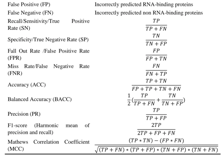
Table 2. Name and definition of the evaluation metric.
Name of Metric Definition
True Positive (TP) Correctly predicted RNA-binding proteins True Negative (TN) Correctly predicted non RNA-binding proteins False Positive (FP) Incorrectly predicted RNA-binding proteins False Negative (FN) Incorrectly predicted non RNA-binding proteins Recall/Sensitivity/True Positive
Rate (SN)
𝑇𝑃 𝑇𝑃 + 𝐹𝑁
Specificity/True Negative Rate (SP) 𝑇𝑁
𝑇𝑁 + 𝐹𝑃 Fall Out Rate /False Positive Rate
(FPR)
𝐹𝑃 𝐹𝑃 + 𝑇𝑁 Miss Rate/False Negative Rate
(FNR)
𝐹𝑁 𝐹𝑁 + 𝑇𝑃
Accuracy (ACC) 𝑇𝑃 + 𝑇𝑁
𝐹𝑃 + 𝑇𝑃 + 𝑇𝑁 + 𝐹𝑁
Balanced Accuracy (BACC) 1
2( 𝑇𝑃 𝑇𝑃 + 𝐹𝑁+ 𝑇𝑁 𝑇𝑁 + 𝐹𝑃) Precision (PR) 𝑇𝑃 𝑇𝑃 + 𝐹𝑃 F1-score (Harmonic mean of
precision and recall)
2𝑇𝑃 2𝑇𝑃 + 𝐹𝑃 + 𝐹𝑁 Mathews Correlation Coefficient
(MCC)
(𝑇𝑃 ∗ 𝑇𝑁) − (𝐹𝑃 ∗ 𝐹𝑁)
23
2.4 Feature Selection
In this section, we discuss the feature selection approaches that we adopted to select relevant features. During the feature extraction process, we collected a feature vector of 2603 dimensions, which is significantly large. Therefore, to reduce the feature space and select the relevant features that could help improve the classification accuracy, we adopted two distinct feature selection approaches, namely Incremental Feature Selection (IFS) and Genetic Algorithm (GA) based feature selection.
Feature Selection using IFS
IFS starts with an empty feature vector and a feature group is added to the feature vector if the addition of the feature group to the feature vector improves the performance of the predictor. In case, by adding the new feature group, the accuracy of the predictor is reduced, this feature group is discarded, and a new feature group is tested in an iterative fashion. During IFS, we performed 10-fold CV on benchmark dataset using XGBoost as a predictor. The values of XGBoost parameters: max_depth, eta, silent, objective, num_class, n_estimators, min_child_weight, subsample, scale_pos_weight, tree_method and max_bin were set to 6, 0.1, 1, ‘multi:softprob’, 2, 100, 5, 0.9, 3, ‘hist’ and 500, respectively and the rest of the parameters were set to their default value. We used ACC as the evaluation metric to decide whether the new feature group will be added to the feature vector or not. In our implementation of IFS, only Vander Waals Volume feature group was ignored from the feature vector as the addition of this feature decreased the ACC of the predictor. Therefore, through IFS, 2582 features out of 2603 features were selected as relevant features.
24
Feature Selection using GA
GA is a population-based stochastic search technique that mimics the natural process of evolution. It contains a population of chromosomes where each chromosome represents a possible solution to the problem under consideration. In general, a GA operates by initializing the population randomly, and by iteratively updating the population through various operators including elitism, crossover and mutation to discover, prioritize and recombine good building blocks present in parent chromosomes to finally obtain fitter chromosome (Hoque, et al., 2010; Hoque, et al., 2007; Hoque and Iqbal, 2017).
Encoding the solution of the problem under consideration in the form of chromosomes and computing the fitness of the chromosomes are two important steps in setting up the GA. Here, to perform feature selection, we encode each feature 𝑓𝑖 in our feature space 𝐹 = [𝑓1, 𝑓2, ⋯ , 𝑓𝑛] by a single bit of 1/0 in a chromosome space where, the value of 1 represents that the i-th feature is selected and the value of 0 represents that the i-th feature is not selected. The length of the chromosome space is equal to the length of the feature space. Moreover, to compute the fitness of the chromosome, we use the XGBoost algorithm (Chen and Guestrin, 2016). The choice of XGBoost was made because of its fast execution time and reasonable performance compared to other machine learning classifiers. During feature selection, the values of XGBoost parameters: max_depth, eta, silent, objective, num_class, n_estimators, min_child_weight, subsample, scale_pos_weight, tree_method, and max_bin were set to 6, 0.1, 1, ‘multi:softprob’, 2, 100, 5, 0.9, 3, ‘hist’ and 500, respectively and the rest of the parameters were set to their default value. In our implementation, the objective fitness is defined as:
25
where, ACC is the accuracy, AUC is the area under the receiver operating characteristic curve and MCC is the Matthews Correlation Coefficient. To evaluate the fitness of the chromosome, a new data space D is obtained which only includes the features for which the chromosome bit is 1. The values of ACC, AUC and MCC metrics of the obj_fit are obtained by performing 10-fold CV on a new data space D using the XGBoost algorithm. Furthermore, the additional parameters of the GA in our implementation were set to a population size of 20, maximum generation to 300, elite-rate to 5%, crossover-elite-rate to 90% and mutation elite-rate to 50%. Through this GA based feature selection, only 1346 features out of 2603 features were selected as relevant features. Therefore, we were able to achieve two-fold benefits from the GA based features selection which are significantly reduced feature space and relevant features. Finally, we noticed that at least one of the features from each type of features we extracted was present in the feature set selected by GA. Therefore, all the feature types extracted in this study were found to be important for the prediction of RBPs.
2.5 Framework of AIRBP
To develop the AIRBP predictor for RBPs prediction, we adopted the idea of a stacking based machine learning approach (Wolpert, 1992) which, has recently been successfully applied to solve various bioinformatics problems (Hu, et al., 2015; Iqbal and Hoque, 2018; Mishra, et al., 2018; Nagi and Bhattacharyya, 2013). Stacking is an ensemble based machine learning approach, which collects information from multiple models in different phases and combines them to form a new model. Stacking is considered to yield more accurate results than the individual machine learning methods as the information gained from more than one predictive model minimizes the generalization error. Stacking framework includes two-levels of classifiers, where the classifiers
26
of the first-level are called base-classifiers and the classifiers of the second-level are called meta-classifiers. In the first level, a set of base-classifiers C1, C2, …, CN are employed (Džeroski and
Ženko, 2004). The prediction probabilities from the base-classifiers are combined using a meta-classifier to reduce the generalization error and improve the accuracy of the predictor. To enrich the meta-classifier with necessary information on the problem space, the classifiers at the base-level are selected such that their underlying operating principles are different from one another (Mishra, et al., 2018; Nagi and Bhattacharyya, 2013).
In order to select the classifiers to use in the first and second level of the AIRBP stacking framework, we analyzed the performance of six individual classification methods: i) Random Decision Forest (RDF) (Ho, 1995); ii) Bagging (Bag) (Breiman, 1996); iii) Extra Tree (ET) (Geurts, et al., 2006); iv) Extreme Gradient Boosting (XGBoost or XGB) (Chen and Guestrin, 2016); v) Logistic Regression (LogReg) (Hastie, et al., 2009; Szilágyi and Skolnick, 2006); and vi) K-Nearest Neighbor (KNN) (Altman, 1992).
All the classification methods mentioned above are built and optimized using python’s Scikit-learn library (Pedregosa, et al., 2012). In order to design stacking framework for AIRBP, we evaluated the different combination of base-classifiers and finally selected the one that provided the highest performance. The set of stacking framework tested are:
i) SF1:RDF, XGBoost, LogReg, KNN in base-level and XGBoost in meta-level, ii)SF2:Bag, XGBoost, LogReg, KNN in base-level and XGBoost in meta-level and iii) SF3:ET, XGBoost, LogReg, KNN in base-level and XGBoost in meta-level.
Here, the choice of base-level classifiers is made such that the underlying principle of learning of each of the classifiers is different from each other (Mishra, et al., 2018). For example, in SF1, SF2 and SF3 the tree-based classifiers RDF, Bag and ET are individually combined with the other two
27
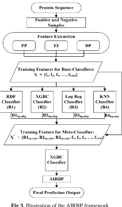
methods LogReg and KNN to learn different information from the problem-space. Additionally, for each of the combination SF1, SF2 and SF3, the XGBoost classifier is used both in the base as well as in the meta-level because it performed best among all the other individual methods applied in this work. While examining the 10-fold CVs performance of the above three combinations, we found that the first stacking framework, SF1 attains the highest performance. Therefore, we employ four classifiers RDF, XGBoost, LogReg, and KNN as the base classifiers and another XGBoost as the meta-classifier in AIRBP stacking framework. In AIRBP, the probabilities of both the classes (RBP and non-RBP) generated by the four base-classifiers are combined with the 1346 features selected by GA and provided as an input features to the meta-classifier which eventually provides the prediction for RBPs. Fig. 3 illustrates the prediction framework of the AIRBP.
28
Fig 3. Illustration of the AIRBP framework.
2.6 Results
In this section, we first demonstrate the results of the feature selection. Then, we show the performance comparison of potential base-classifiers and stacking frameworks. Finally, we report the performance of AIRBP on the benchmark dataset and three independent test datasets and consequently compare it with the existing method.
29
2.6.1Feature Selection
To reduce the feature space and select the relevant features that support the classification accuracy, we adopted the IFS and GA based feature selection approach. Through IFS and GA, 2582 and 1346 features out of 2603 total features were selected as relevant features, respectively. From Table 3, we observe that IFS could not reduce the feature space as significantly as GA. Additionally, the performance of XGBoost after IFS did not improve significantly and is lower than the performance resulted by the GA-based feature selection. We found that the benefit of GA feature selection were two folds, significant reduction of feature space and identification of relevant features along with improved performance. In Supplementary Table 3S, we show the performance comparison of XGBoost based predictor before and after IFS and GA-based feature selection.
Table 3. Comparison of RBPs prediction results on benchmark dataset before and after feature selection. Algorithm Num. of Features Evaluation Metrics SN (%) SP (%) BACC (%) ACC (%) FPR FNR PR (%) F1-score MCC XGBoost Before Feature Selection 2603 82.11 96.81 89.46 92.64 0.03 0.18 91.06 0.86 0.82 XGBoost After IFS 2582 82.26 96.92 89.59 92.76 0.03 0.18 91.37 0.87 0.82 XGBoost After GA-based Feature Selection 1346 89.13 96.95 91.03 93.59 0.03 0.15 91.71 0.88 0.84
30
2.6.2 Selection of Classifiers for Stacking
To select the methods to use as the base and the meta-classifiers, we analyzed the performance of six different machine learning algorithms: RDF, Bag, ET, XGBoost, LogReg, and KNN on the benchmark dataset through 10-fold CV approach. The performance comparison of the individual classifiers on the benchmark dataset is shown in Table 4.
Table 4. Comparison of various machine learning algorithms on the benchmark dataset through 10-fold CV.
Metric/Methods Bag KNN LogReg RDF XGBoost ET
SN (%) 82.18 57.54 82.00 72.24 89.09 67.44 SP (%) 96.84 89.17 96.39 98.47 97.48 98.58 BACC (%) 89.51 73.35 89.20 85.36 93.28 83.01 ACC (%) 92.68 80.19 92.31 91.03 95.10 89.75 FPR 0.032 0.108 0.036 0.015 0.025 0.014 FNR 0.178 0.425 0.180 0.278 0.109 0.326 PR (%) 91.14 67.77 90.00 94.92 93.34 94.96 F1-score 0.866 0.622 0.858 0.820 0.912 0.789 MCC 0.816 0.492 0.807 0.775 0.878 0.742
Best score values are bold faced.
Table 4 further shows that the optimized XGBoost is the best performing classifier among six different classifiers implemented in our study, in terms of sensitivity, balanced accuracy, accuracy, FNR, F1-score, and MCC. Moreover, the optimized XGBoost attains sensitivity, balanced accuracy, accuracy, FNR, F1-score, and MCC of 89.09%, 93.28%, 0.109, 0.912, and 0.878, respectively. Besides, the ET classifier attains the highest specificity, FPR, and precision of 98.58%, 0.014, and 94.96%, respectively. As the benchmark dataset is highly imbalanced, we consider MCC as the deciding scores as it provides the balanced measure of any predictor trained on an imbalanced dataset. Furthermore, it is evident from Table 1 that the MCC of the optimized XGBoost is 18.33%, 13.29%, 8.79%, 78.46%, and 7.59% higher than ET, RDF, LogReg, KNN,
31
and Bag, respectively. The greater performance of the XGBoost algorithm motivated us to use it both as a base as well as a meta-classier in the AIRBP prediction framework.
To further select the classifiers to be used at the level, we adopted the guidelines of base-classifier selection based on different underlying principles. Therefore, we used KNN and LogReg as two additional classifiers at the base-level. Then, we added single tree-based ensemble method out of three methods, RDF, Bag, and ET, at a time as the fourth base-classifier and designed three different combinations of stacking framework, namely SF1, SF2, and SF3. The performance comparison of SF1, SF2 and SF3 stacking framework on the benchmark dataset using 10-fold CV are presented in Table 5.
Table 5. Comparison of different stacking framework with different set of base-classifiers on benchmark dataset through 10-fold CV.
Metric/Methods SF1 SF2 SF3 SN (%) 90.17 89.99 90.53 SP (%) 97.44 97.15 97.29 BACC (%) 93.80 93.57 93.91 ACC (%) 95.38 95.12 95.38 FPR 0.026 0.028 0.027 FNR 0.098 0.100 0.095 PR (%) 93.31 92.59 92.98 F1-score 0.917 0.912 0.917 MCC 0.885 0.879 0.885
Best scores are bold faced.
Table 5 demonstrates that SF1, which includes RDF, XGBoost, LogReg, and KNN as base-classifiers and another XGBoost as a meta-classifier outperformed SF2 and SF3. Hence, we select SF1 as our final predictor of RBPs.
32
2.6.3 Performance Comparison with Existing Approaches on the Benchmark Dataset
Here, we compare the performance of AIRBP with RBPPred (Zhang and Liu, 2017) on the benchmark dataset using the 10-fold CV approach. RBPPred is a top performing existing approach for the prediction of RBPs directly from the sequence. Furthermore, it is to be noted that AIRBP uses the same benchmark dataset as RBPPred therefore, for the comparison, the quantities for all the evaluation metrics for RBPPred are obtained from Zhang and Liu (Zhang and Liu, 2017). The prediction results of AIRBP and RBPPred on benchmark dataset computed using 10-fold CV are listed in Table 6.
Table 6. Comparison of AIRBP with existing method on benchmark dataset through 10-fold CV.
Metric/Methods RBPPred AIRBP (% imp.)
SN (%) 83.07 90.17 (8.55%) SP (%) 96.00 97.44 (1.50%) BACC (%) - 93.80 (-) ACC (%) 92.36 95.38 (3.26%) FPR - 0.026 (-) FNR - 0.098 (-) PR (%) 89.00 93.31 (4.84%) F1-score 0.859 0.917 (6.75%) MCC 0.808 0.885 (9.53%)
Here, best scores are bold faced. The ‘% imp.’ stands for percentage improvement and ‘-’ represents missing value or the value not reported by RBPPred and ‘(-)’ represents that the % imp. cannot be calculated.
From Table 6, we observed that AIRBP outperforms RBPPred based on all the evaluation metrics applied in this study. Particularly, AIRBP provides 8.55%, 1.50%, 3.26%, 4.84%, 6.75% and 9.53% improvement over RBPPred based on SN, SP, ACC, PR, F1-score and MCC, respectively. In addition, in Table 3, we report the values of BACC, FPR, and FNR only for the AIRBP predictor as the values of these metrics were not reported by RBPPred. Since our benchmark dataset is highly imbalanced (contains 2767 RBPs and 6987 non-RBPs) which also reflects the natural frequency, we focus on comparing the predictors based on MCC and F1-score. MCC considers true and false
33
positives as well as negatives and is generally considered as a balanced measure which can be used even though the classes are of very different sizes. Likewise, F1-score is the harmonic average of the precision and recall and is generally considered another balanced measure when the dataset is imbalanced. Since F1-score considers harmonic average, it is considered to provide an appropriate score to the model rather than an arithmetic mean. From Table 3, it is clear that based on MCC and F1-score AIRBP outperforms RBPPred by 9.53% and 6.75%.
2.6.4 Performance Comparison with Existing Approaches on the Independent Test Set
In this section, we further compare the performance of AIRBP with RBPPred predictor on three different independent test sets, Human, S. cerevisiae and A. thaliana. Here, we only report the comparison of AIRBP with RBPPred because RBPPred is the top performing sequence-based predictor of RBPs in the literature. As reported, RBPPred provides much better performance than SPOT-seq (Zhao, et al., 2011) and RNApred (Kumar, et al., 2011) predictors, which are the only two additional sequence-based methods that can be accessed either through a web server or code is publicly available for download. To perform independent testing, we first train AIRBP on complete benchmark dataset and subsequently test it on three different independent test sets, Human, S. cerevisiae and A. thaliana. The predictive results of AIRBP and RBPPred on three different independent test sets are compared in Table 4. Table 4 indicates that AIRBP achieves an improvement of 9.32% in SN, 4.54% in ACC, 4.19% in F1-score and 8.50% in MCC over RBPPred on Human test set. Likewise, AIRBP achieves an improvement of 9.51% in SN, 4.41% in ACC, 3.52% in F1-score and 8.23% in MCC over RBPPred on S. cerevisiae test set. Furthermore, while testing on A. thaliana, AIRBP achieves an improvement of 6.61% in SN, 5.34% in ACC, 4.28% in PR, 3.03% in F1-score and 10.61% in MCC over RBPPred approach.
34
Moreover, while analyzing the average percentage improvement over all the independent test sets AIRBP attains improvement of 8.48% in SN, 4.76% in ACC, 0.21% in PR, 3.58% in F1-score and 9.11% in MCC over RBPPred. Besides, RBPPred seems to be 7.34% better in an average over three test sets in terms of SP (i.e. predicting negative samples or non-RBPs) over AIRBP. However, AIRBP provides 0.21% improvement in an average over three test sets in terms of PR over RBPPred. Additionally, as stated above, for the imbalanced dataset the F1-score and MCC are widely used as a balanced measure between sensitivity and specificity. Our predictor, AIRBP shows consistent improvement in F1-score and MCC over RBPPred for all three independent test set. Specifically, AIRBP provides 4.19% and 8.05% improvement in F1-score and MCC, respectively over RBPPred while tested on Human test set. Similarly, AIRBP shows 3.52% and 8.23% improvement in F1-score and MCC, respectively over RBPPred on S. cerevisiae as well as 3.03% and 10.61% improvement in F1-score and MCC, respectively over RBPPred on A. thaliana
Table 7: Comparison of AIRBP with an existing method using independent test sets.
Meth ods Dataset Evaluation Metrics SN (%) SP (%) BACC (%) ACC (%) FPR FNR PR (%) F1-score MCC RBP Pred Human 84.28 96.65 - 89.00 - - 97.65 0.905 0.788 S. cerevisiae 86.16 94.59 - 87.73 - - 96.52 0.910 0.729 A. thaliana 86.40 94.59 - 87.02 - - 94.59 0.925 0.537 AIR BP Human (% imp.) 92.14 (9.32%) 94.52 (-2.21%) 93.33 (-) 93.04 (4.54%) 0.055 (-) 0.079 (-) 96.53 (-1.14%) 0.943 (4.19%) 0.855 (8.50%) S. cerevisiae (% imp.) 94.35 (9.51%) 84.33 (-10.85%) 89.34 (-) 91.60 (4.41%) 0.157 (-) 0.057 (-) 94.09 (-2.52%) 0.942 (3.52%) 0.789 (8.23%) A. thaliana (% imp.) 92.11 (6.61%) 86.11 (-8.97%) 89.11 (-) 91.67 (5.34%) 0.139 (-) 0.079 (-) 98.82 (4.28%) 0.953 (3.03%) 0.594 (10.61%) (avg.% imp.) (8.48%) (-7.34%) (-) (4.76) (-) (-) (0.21%) (3.58%) (9.11%)
Here, ‘imp.’ stands for improvement. The ‘% imp.’ represents the improvement in percentage achieved by AIRBP for corresponding independent test set for corresponding evaluation metric over the RBPPred method. Likewise, the ‘avg. % imp.’ represents the average percentage improvement achieved by AIRBP for all independent test set for corresponding evaluation metric over the RBPPred method. Additionally, ‘-’ represents missing value or the value not reported by RBPPred and ‘(-)’ represents that the % imp. or avg. % imp. cannot be calculated.
35
test set. Finally, based on an average percentage improvement (calculated over three different datasets) in F1-score and MCC, AIRBP outperforms RBPPred by 3.58% and 9.11%.
The above comparison of results indicates that the proposed method, AIRBP outperforms the existing methods and is a very promising predictor. We believe that this comprehensive investigation of the stacking based machine learning framework and features in predicting RNA binding proteins might be useful for future proteomics studies.
2.7 Conclusions
In this work, we constructed a stacking based machine learning framework, called AIRBP, for the prediction of RNA-binding proteins directly from the protein sequence. To improve the prediction accuracy of RNA-binding proteins, we have investigated and used various feature extraction and encoding techniques, various feature selection techniques along with an advanced machine learning technique called stacking. We extracted various features including evolutionary information, physiochemical properties, and disordered properties and applied various encoding techniques such as composition, transition and distribution, conjoint triad, PSSM distance transformation, and residue-wise contact energy matrix transformation to encode the protein sequence in terms of features. Next, we applied two different feature selection techniques incremental feature selection and genetic algorithm based feature selection to identify the relevant features as well as to significantly reduce the feature space. Next, only the relevant features are used to train the ensemble of predictors at the first-level (i.e. base-layer) of the stacking framework. Then, the prediction probabilities from the first-level predictors are combined with the originally selected features and used to train the predictor at the second-level (i.e. meta-layer) of the stacking framework. Finally, the AIRBP stacking framework achieves a 10-fold CV accuracy, F1-score,
36
and MCC of 95.38%, 0.917 and 0.885 respectively, on the benchmark dataset. While performing the independent test, AIRBP achieves an accuracy, F1-score, and MCC of 93.04%, 0.943 and 0.855, for Human test set; 91.60%, 0.942 and 0.789 for S. cerevisiae test set; and 91.67%, 0.953 and 0.594 for A. thaliana test set, respectively. These promising results indicate that the stacking framework helps improve the accuracy significantly by reducing the generalization error. Furthermore, in comparison with the top performing method, RBPPred, AIRBP achieves 3.26%, 6.75% and 9.53% improvement in terms of accuracy, F1-score and MCC respectively, based on a benchmark dataset. F1-score and MCC are two widely used measures for the imbalanced dataset. Moreover, the average percentage improvement, calculated over three different independent test sets, AIRBP outperforms RBPPred by 4.76%, 3.58% and 9.11% in terms of accuracy, F1-score, and MCC, respectively. These outcomes help us summarize that the AIRBP can be effectively used for accurate and fast identification and annotation of RNA-binding proteins directly from the protein sequence and can provide valuable insights for treating critical diseases.