See the Tree Through the Lines:
The Shazoo Algorithm
Fabio Vitale
DSI, University of Milan, Italy [email protected]
Nicol`o Cesa-Bianchi DSI, University of Milan, Italy [email protected]
Claudio Gentile
DICOM, University of Insubria, Italy [email protected]
Giovanni Zappella
Department of Mathematics, University of Milan, Italy [email protected]
Abstract
Predicting the nodes of a given graph is a fascinating theoretical problem with ap-plications in several domains. Since graph sparsification via spanning trees retains enough information while making the task much easier, trees are an important special case of this problem. Although it is known how to predict the nodes of an unweighted tree in a nearly optimal way, in the weighted case a fully satisfactory algorithm is not available yet. We fill this hole and introduce an efficient node predictor, SHAZOO, which is nearly optimal on any weighted tree. Moreover, we show that SHAZOOcan be viewed as a common nontrivial generalization of both
previous approaches for unweighted trees and weighted lines. Experiments on real-world datasets confirm that SHAZOOperforms well in that it fully exploits the structure of the input tree, and gets very close to (and sometimes better than) less scalable energy minimization methods.
1
Introduction
Predictive analysis of networked data is a fast-growing research area whose application domains include document networks, online social networks, and biological networks. In this work we view networked data as weighted graphs, and focus on the task of node classification in the transductive setting, i.e., when the unlabeled graph is available beforehand. Standard transductive classification methods, such as label propagation [2, 3, 18], work by optimizing a cost or energy function defined on the graph, which includes the training information as labels assigned to training nodes. Although these methods perform well in practice, they are often computationally expensive, and have perfor-mance guarantees that require statistical assumptions on the selection of the training nodes. A general approach to sidestep the above computational issues is to sparsify the graph to the largest possible extent, while retaining much of its spectral properties —see, e.g., [5, 6, 12, 16]. Inspired by [5, 6], this paper reduces the problem of node classification from graphs to trees by extracting suitablespanning treesof the graph, which can be done quickly in many cases. The advantage of performing this reduction is that node prediction is much easier on trees than on graphs. This fact has recently led to the design of very scalable algorithms with nearly optimal performance guarantees in the online transductive model, which comes with no statistical assumptions. Yet, the current results in node classification on trees are not satisfactory. The TREEOPTstrategy of [5] is optimal to within constant factors, but only onunweightedtrees. No equivalent optimality results are available for general weighted trees. In fact, WTAcan still be applied to weighted trees by exploiting an idea
contained in [9]. This is based on linearizing the tree via a depth-first visit. Since linearization loses most of the structural information of the tree, this approach yields suboptimal mistake bounds. This theoretical drawback is also confirmed by empirical performance: throwing away the tree structure negatively affects the practical behavior of the algorithm on real-world weighted graphs.
The importance of weighted graphs, as opposed to unweighted ones, is suggested by many practical scenarios where the nodes carry more information than just labels, e.g., vectors of feature values. A natural way of leveraging this side information is to set the weight on the edge linking two nodes to be some function of the similariy between the vectors associated with these nodes. In this work, we bridge the gap between the weighted and unweighted cases by proposing a new prediction strategy, called SHAZOO, achieving a mistake bound that depends on the detailed structure of the weighted tree. We carry out the analysis using a notion of learning bias different from the one used in [6] and more appropriate for weighted graphs. More precisely, we measure the regularity of the unknown node labeling via the weighted cutsize induced by the labeling on the tree (see Section 3 for a precise definition). This replaces the unweighted cutsize that was used in the analysis ofWTA. When the weighted cutsize is used, a cut edge violates this inductive bias in proportion to its weight. This modified bias does not prevent a fair comparison between the old algorithms and the new one: SHAZOO specializes to TREEOPT in the unweighted case, and to WTA when the input tree is a weighted line. By specializing SHAZOO’s analysis to the unweighted case we recover TREEOPT’s optimal mistake bound. When the input tree is a weighted line, we recoverWTA’s mistake bound expressed through the weighted cutsize instead of the unweighted one. The effectiveness of SHAZOO
on any tree is guaranteed by a corresponding lower bound (see Section 3).
SHAZOOcan be viewed as a common nontrivial generalization of both TREEOPTandWTA. Obtain-ing this generalization while retainObtain-ing and extendObtain-ing the optimality properties of the two algorithms is far from being trivial from a conceptual and technical standpoint. Since SHAZOOworks in the online transductive model, it can easily be applied to the more standard train/test (or “batch”) trans-ductive setting: one simply runs the algorithm on an arbitrary permutation of the training nodes, and obtains a predictive model for all test nodes. However, the implementation might take advantage of knowing the set of training nodes beforehand. For this reason, we present two implementations of SHAZOO, one for the online and one for the batch setting. Both implementations result in fast algorithms. In particular, the batch one is linear in|V|. This is achieved by a fast algorithm for weighted cut minimization on trees, a procedure which lies at the heart of SHAZOO.
Finally, we test SHAZOO against WTA, label propagation, and other competitors on real-world weighted graphs. Inalmost allcases (as expected), we report improvements overWTAdue to the bet-ter sensitivity to the graph structure. In some cases, we see that SHAZOOeven outperforms standard label propagation methods. Recall that label propagation has a running time per prediction which is proportional to|E|, whereEis the graph edge set. On the contrary, SHAZOOcan be typically run in constantamortized time per prediction by using Wilson’s algorithm for sampling random spanning trees [17]. By disregarding edge weights in the initial sampling phase, this algorithm is able to draw a random (unweighted) spanning tree in time proportional to|V|on most graphs. Our experiments reveal that using the edge weights only in the subsequent prediction phase causes in practice only a minor performance degradation.
2
Preliminaries and basic notation
LetT = (V, E, W)be an undirected and weighted tree with|V|=nnodes, positive edge weights
Wi,j >0for(i, j)∈ E, andWi,j = 0for(i, j) ∈/ E. A binary labeling ofT is any assignment
y= (y1, . . . , yn)∈ {−1,+1}nof binary labels to its nodes. We use(T,y)to denote the resulting
labeled weighted tree. The online learning protocol for predicting(T,y)is defined as follows. The learner is givenT whileyis kept hidden. The nodes ofT are presented to the learner one by one, according to an unknown and arbitrary permutationi1, . . . , inofV. At each time stept= 1, . . . , n
nodeitis presented and the learner must issue a predictionybit ∈ {−1,+1}for the labelyit. Then
yitis revealed and the learner knows whether a mistake occurred. The learner’s goal is to minimize the total number of prediction mistakes.
Following previous works [10, 9, 5, 6], we measure the regularity of a labelingyofT in terms of
φ-edges, where aφ-edge for(T,y)is any(i, j) ∈ E such thatyi 6= yj. The overall amount of
irregularity in a labeled tree(T,y)is theweighted cutsizeΦW =P
(i,j)∈EφWi,j, whereEφ⊆E
want to design algorithms whose predictive performance scales withΦW. Unlike theφ-edge count
Φ =|Eφ|, which is a good measure of regularity for unweighted graphs, the weighted cutsize takes the edge weightWi,jinto account when measuring the irregularity of aφ-edge(i, j). In the sequel,
when we measure the distance between any pair of nodesiandjon the input treeT we always use the resistance distance metricd. That is, d(i, j) = P
(r,s)∈π(i,j) 1
Wr,s, whereπ(i, j)is the unique path connectingitoj.
3
A lower bound for weighted trees
In this section we show that the weighted cutsize can be used as a lower bound on the number of online mistakes made by any algorithm on any tree. In order to do so (and unlike previous papers on this specific subject —see, e.g., [6]), we need to introduce a more refined notion of adversarial “budget”. GivenT = (V, E, W), letξ(M)be the maximum number of edges ofT such that the sum of their weights does not exceedM,ξ(M) = maxn|E0| : E0⊆E, P
(i,j)∈E0wi,j≤M
o
.
We have the following simple lower bound, whose proof is provided in the supplementary material to this paper.
Theorem 1 For any weighted treeT = (V, E, W)there exists a randomized label assignment to
V such that any algorithm can be forced to make at leastξ(M)/2online mistakes in expectation, whileΦW ≤M.
Specializing [6, Theorem 1] to trees gives the lower boundK/2under the constraintΦ≤K≤ |V|. The main difference between the two bounds is the measure of label regularity being used: Whereas Theorem 1 usesΦW, which depends on the weights, [6, Theorem 1] uses the weight-independent
quantityΦ. This dependence of the lower bound on the edge weights is consistent with our learning bias, stating that a heavyφ-edge violates the bias more than a light one.
Since ξ is a nondecreasing function, the lower bound implies a number of mistakes of at least
ξ(ΦW)/2. Note that ξ(ΦW) ≥ Φ for any labeled tree (T,y). Hence, whereas a constraintK
onΦimplies forcing at leastK/2mistakes, a constraintM onΦW allows the adversary to force a
potentially larger number of mistakes.
In the next section we describe an algorithm whose mistake bound nearly matches the above lower bound on any weighted tree when usingξ(ΦW)as the measure of label regularity.
Algorithm 1:SHAZOO
fort= 1. . . n
LetC H(it)
be the set of the connection nodesiofH(it)for which∆(i)6= 0
ifC H(it)
6≡ ∅
Letjbe the node ofC H(it)
closest toit
Setbyit = sgn ∆(j)
else
Setbyit =−1(default value)
4
The Shazoo algorithm
In this section we introduce the SHAZOOalgorithm, and relate it to previously proposed methods for online prediction on unweighted trees (TREEOPTfrom [5]) and weighted line graphs (WTAfrom [6]). In fact, SHAZOOis optimal on any weighted tree, and reduces to TREEOPTon unweighted trees and toWTAon weighted line graphs. Since TREEOPTandWTAare optimal onanyunweighted tree andanyweighted line graph, respectively, SHAZOOnecessarily contains elements of both of these algorithms.
In order to understand our algorithm, we now define some relevant structures of the input treeT. These structures evolve over time according to the set of observed labels. First, we callrevealeda node whose label has already been observed by the online learner; otherwise, a node isunrevealed. Aforkis any unrevealed node connected to at least three different revealed nodes by edge-disjoint
paths. Ahinge nodeis either a revealed node or a fork. Ahinge treeis any component of the forest obtained by removing fromT alledges incident to hinge nodes; hence any fork or labeled node forms a1-node hinge tree. When a hinge treeH contains only one hinge node, aconnection node forH is the node contained inH. In all other cases, we call a connection node forH any node outsideH which is adjacent to a node inH. Aconnection forkis a connection node which is also a fork. Finally, ahinge lineis any path connecting two hinge nodes such that no internal node is a hinge node. See Figure 1 (left) for an example.
1 2 1 3 2 4 2 1 1 1 2 1 >0 >0 <0 + + + + + 2 4 3 6 1 5 1+a 1+2a 1+(V-1)a 1+3a
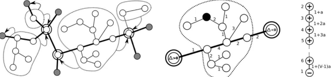
Figure 1: Left: An input tree. Revealed nodes are dark grey, forks are doubly circled, and hinge lines have thick black edges. The hinge trees not containing hinge nodes (i.e., the ones that are not singletons) are enclosed by dotted lines. The dotted arrows point to the connection node(s) of such hinge trees.Middle:The predictions of SHAZOOon the nodes of a hinge tree. The numbers on the edges denote edge weights. At a given timet, SHAZOOuses the value of∆on the two hinge nodes (the doubly circled ones, which are also forks in this case), and is required to issue a prediction on nodeit(the black node in this figure). Sinceitis between a positive∆hinge node and a negative
∆hinge node, SHAZOOgoes with the one which is closer in resistance distance, hence predicting
b
yit=−1.Right:A simple example where the mincut prediction strategy does not work well in the weighted case. In this example, mincut mispredicts all labels, yetΦ = 1, and the ratio ofΦW to the
total weight of all edges is about1/|V|. The labels to be predicted are presented according to the numbers on the left of each node. Edge weights are also displayed, whereais a very small constant. Given an unrevealed nodeiand a label valuey∈ {−1,+1}, thecut functioncut(i, y)is the value of the minimum weighted cutsize ofT over all labelingsy∈ {−1,+1}nconsistent with the labels
seen so far and such thatyi =y. Define∆(i) = cut(i,+1)−cut(i,−1)ifiis unrevealed, and
∆(i) = yi, otherwise. The algorithm’s pseudocode is given in Algorithm 1. At timet, in order
to predict the labelyit of nodeit, SHAZOO calculates∆(i)for all connection nodes iof H(it), whereH(it)is the hinge tree containingit. Then the algorithm predictsyit using the label of the connection nodeiofH(it)which is closest toitand such that∆(i) 6= 0(recall from Section 2
that all distances/lengths are measured using the resistance metric). Ties are broken arbitrarily. If ∆(i) = 0 for all connection nodesiinH(it)then SHAZOOpredicts a default value (−1 in the
pseudocode). Ifit is a fork (which is also a hinge node), thenH(it) = {it}. In this case,itis
a connection node ofH(it), and obviously the one closest to itself. Hence, in this case SHAZOO
predictsytsimply byybit = sgn ∆(it)
. See Figure 1 (middle) for an example.
On unweighted trees, computing∆(i)for a connection nodeireduces to the Fork Label Estima-tion Procedure in [5, Lemma 13]. On the other hand, predicting with the label of the connecEstima-tion node closest toitin resistance distance is reminiscent of the nearest-neighbor prediction ofWTA
on weighted line graphs [6]. In fact, as inWTA, this enables to take advantage of labelings whose
φ-edges are light weighted. An important limitation ofWTAis that this algorithm linearizes the in-put tree. On the one hand, this greatly simplifies the analysis of nearest-neighbor prediction; on the other hand, this prevents exploiting the structure ofT, thereby causing logaritmic slacks in the upper bound ofWTA. The TREEOPTalgorithm, instead, performs better when the unweighted input tree is very different from a line graph (more precisely, when the input tree cannot be decomposed into long edge-disjoint paths, e.g., a star graph). Indeed, TREEOPTupper bound does not suffer from logaritmic slacks, and is tight within constant factors on any unweighted tree. Similar to TREEOPT, SHAZOO does not linearize the input tree and extends to the weighted case TREEOPT’s superior performance, also confirmed by the experimental comparison reported in Section 7.
In Figure 1 (right) we show an example that highlights the importance of using the∆function to compute the fork labels. Since∆predicts a forkitwith the label that minimizes the weighted cutsize
based on the number ofφ-edges (rather than their weighted sum) could be an effective prediction strategy. Figure 1 (right) illustrates an example of a simple tree where such a∆ mispredicts the labels of all nodes, when bothΦW andΦare small.
Remark 1 We would like to stress thatSHAZOOcan also be used to predict the nodes of an arbi-trarygraphby first drawing a random spanning treeT of the graph, and then predicting optimally onT —see, e.g., [5, 6]. The resulting mistake bound is simply the expected value of SHAZOO’s mistake bound over the random draw ofT. By using a fast spanning tree sampler [17], the involved computational overhead amounts to constant amortized time per node prediction on “most” graphs. Remark 2 In certain real-world input graphs, the presence of an edge linking two nodes may also carry information about the extent to which the two nodes aredissimilar, rather than similar. This information can be encoded by the sign of the weight, and the resulting network is called asigned
graph. The regularity measure is naturally extended to signed graphs by counting the weight of
frustrated edges (e.g.,[7]), where (i, j)is frustrated if yiyj 6= sgn(wi,j). Many of the existing
algorithms for node classification [18, 9, 10, 5, 8, 6] can in principle be run on signed graphs. However, the computational cost may not always be preserved. For example, mincut [4] is in general NP-hard when the graph is signed [13]. Since our algorithm sparsifies the graph using trees, it can be run efficiently even in the signed case. We just need to re-define the ∆ function as∆(i) = fcut(i,+1)−fcut(i,−1), where fcutis the minimum total weight of frustrated edges consistent with the labels seen so far. The argument contained in Section 6 for the positive edge weights (see, e.g., Eq. (1) therein) allows us to show that also this version of∆can be computed efficiently. The prediction rule has to be re-defined as well: We count the parity of the numberzof negative-weighted edges along the path connectingitto the closest nodej∈C H(it)
, i.e.,ybit= (−1)
zsgn ∆(j)
. Remark 3 In [5] the authors note thatTREEOPTapproximates a version space (Halving) algo-rithm on the set of tree labelings. Interestingly,SHAZOOis also an approximation to a more general Halving algorithm for weighted trees. This generalized Halving gives a weight to each labeling consistent with the labels seen so far and with the sign of∆(f)for each forkf. These weighted labelings, which depend on the weights of theφ-edges generated by each labeling, are used for com-puting the predictions. One can show (details omitted due to space limitations) that this generalized Halving algorithm has a mistake bound within a constant factor of SHAZOO’s.
5
Mistake bound analysis
We now show that SHAZOOis nearly optimal on every weighted treeT. We obtain an upper bound in terms ofΦW and the structure ofT, nearly matching the lower bound of Theorem 1. Due to its
length, the proof is contained in the supplementary material to this paper. In this section we just give some auxiliary notation that is strictly needed for stating the mistake bound.
Given a labeled tree(T,y), aclusteris any maximal subtree whose nodes have the same label. An in-cluster line graphis any line graph that is entirely contained in a single cluster. Finally, given a line graphL, we setRW
L =
P
(i,j)∈L
1
Wi,j, i.e., the (resistance) distance betweeniandj. Theorem 2 For any labeled and weighted tree(T,y), there exists a setLT ofO ξ(ΦW)
edge-disjoint in-cluster line graphs such that the number of mistakes made bySHAZOOis at most of the order of X L∈LT minn|L|,1 +log 1 + ΦWRWL o .
The above mistake bound depends on the tree structure throughLT. The sum containsO ξ(ΦW)
terms, each one at most logarithmic in the scale-free productsΦWRW
L. The bound is governed by
the same key quantityξ ΦWoccurring in the lower bound of Theorem 1. However, Theorem 2 also shows that SHAZOOcan take advantage of trees that cannot be covered by long line graphs. For example, if the input treeTis a weighted line graph, then it is likely to contain long in-cluster lines. Hence, the factor multiplyingξ ΦW
may be of the order oflog 1 + ΦWRW L
. If, instead,T has constant diameter (e.g., a star graph), then the in-cluster lines can only contain a constant number of nodes, and the number of mistakes can never exceedO ξ(ΦW)
. This is a log factor improvement overWTAwhich, by its very nature, cannot exploit the structure of the tree it operates on.
6
Implementation
We start by describing a method for calculatingcut(v, y)for any unlabeled nodevand label valuey. LetTvbe the maximal subtree ofT rooted atv, such that no internal node is revealed. For any node
iofTv, letTv
i be the subtree ofTvrooted ati. LetΦvi(y)be the minimum weighted cutsize ofTiv
consistent with the revealed nodes and such thatyi=y. Since∆(v) = cut(v,+1)−cut(v,−1) =
Φv
v(+1)−Φvv(−1), our goal is to computeΦvv(y). It is easy to see by induction that the quantity
Φvi(y)can be recursively defined as follows:1
Φvi(y) = X j∈Cv i min y0∈Y j Φvj(y0) +I{y06=y}wi,j ifiis an internal node ofTv 0 otherwise. (1)
HereCivis the set of all children ofiinTv, andYj ≡ {yj}ifyj is revealed, andYj ≡ {−1,+1}
otherwise. NowΦv
v(y)can be computed through a simple depth-first visit ofTv. In all backtracking steps of
this visit the algorithm uses (1) to computeΦv
i(y)for each nodei, the valuesΦvj(y)for all children
jofibeing calculated during the previous backtracking steps. The total running time is therefore linear in the number of nodes ofTv.
Next, we describe the basic implementation of SHAZOOfor the on-line setting. A batch learning implementation will be given at the end of this section. The online implementation is made up of three steps.
1. Find the hinge nodes of subtreeTit. Recall that a hinge-node is either a fork or a revealed node. Observe that a fork is incident to at least three nodes lying on different hinge lines. Hence, in this step we perform a depth-first visit ofTit, marking each node lying on a hinge line. In order to accomplish this task, it suffices to single out all forks marking each labeled node and, recursively, each parent of a marked node ofTit. At the end of this process we are able to single out the forks by counting the number of edges(i, j)of each marked nodeisuch thatjhas been marked, too. The remaining hinge nodes are the leaves ofTitwhose labels have currently been revealed.
2. Computesgn(∆(i))for all connection forks ofH(it). From the previous step we can easily
find the connection node(s) ofH(it). Then, we simply exploit the above-described technique for
computing the cut function, obtainingsgn(∆(i))for all connection forksiofH(it).
3. Propagate the labels of the nodes ofC(H(it))(only ifitis not a fork). We perform a visit of
H(it)starting from every noder∈C(H(it)). During these visits, we mark each nodej ofH(it)
with the label ofrcomputed in the previous step, together with the length ofπ(r, j), which is what we need for predicting any label ofH(it)at the current time step.
The overall running time is dominated by the first step and the calculation of∆(i). Hence the worst case running time is proportional toP
t≤|V||V(Tit)|. This quantity can be quadratic in|V|, though
this is rarely encountered in practice if the node presentation order is not adversarial. For example, it is easy to show that in a line graph, if the node presentation order is random, then the total time is of the order of|V|log2|V|. For a star graph the total time complexity is always linear in|V|, even
on adversarial orders.
In many real-world scenarios, one is interested in the more standard problem of predicting the labels of a given subset oftestnodes based on the available labels of another subset oftrainingnodes. Building on the above on-line implementation, in this section we derive an implementation of SHA -ZOO for this train/test (or “batch learning”) setting. We first show that computing|Φii(+1)|and |Φi
i(−1)|for all unlabeled nodesiinT takesO(|V|)time. This allows us to computesgn(∆(v))
for all forksvinO(|V|)time, and then use the first and the third steps of the on-line implementation. Overall, we show that predictingalllabels in the test set takesO(|V|)time.
Consider treeTi as rooted ati. Given any unlabeled nodei, we perform a visit ofTistarting at
i. During the backtracking steps of this visit we use (1) to calculateΦi
j(y)for each nodej inTi
and labely ∈ {−1,+1}. Observe now that for any pairi, jof adjacent unlabeled nodes and any labely∈ {−1,+1}, once we have obtainedΦii(y),Φji(+1)andΦij(−1), we can computeΦji(y)in
1
constant time, asΦji(y) = Φi
i(y)−miny0∈{−1,+1} Φij(y0) +I{y06=y}wi,j. In fact, all children of j inTi are descendants ofi, while the children of iinTi (butj) are descendants ofj inTj.
SHAZOOcomputesΦii(y), we can compute in constant timeΦij(y)for all child nodesj ofiinTi, and use this value for computingΦjj(y). Generalizing this argument, it is easy to see that in the next phase we can computeΦkk(y)in constant time for all nodeskofTi such that for all ancestorsuof
kand ally∈ {−1,+1}, the values ofΦu
u(y)have previously been computed.
The time for computingΦss(y)for all nodessofTi and any labelyis therefore linear in the time
of performing a breadth-first (or depth-first) visit ofTi, i.e., linear in the number of nodes ofTi.
Since each labeled node with degreedis part of at mostdtreesTifor somei, we have that the total
number of nodes of all distinct (edge-disjoint) treesTiacrossi∈V is linear in|V|.
Finally, we need to propagate the connection node labels of each hinge tree as in the third step of the online implementation. Since this last step takes also linear time, we conclude that the total time for predicting all labels is linear in|V|.
7
Experiments
We tested our algorithm on a number of real-world weighted graphs from different domains (char-acter recognition, text categorization, bioinformatics, Web spam detection) against the following baselines:
Online Majority Vote(OMV). This is an intuitive and fast algorithm for sequentially predicting the node labels is via a weighted majority vote over the labels of the adjacent nodes seen so far. Namely,
OMVpredictsyitthrough the sign of
P
syiswis,it, wheresranges overs < tsuch that(is, it)∈E. Both the total time and space required byOMVareΘ(|E|).
Label Propagation(LABPROP). LABPROP[18, 2, 3] is a batch transductive learning method com-puted by solving a system of linear equations which requires total time of the order of|E|×|V|. This relatively high computational cost should be taken into account when comparing LABPROPto faster online algorithms. Recall thatOMVcan be viewed as a fast “online approximation” to LABPROP. Weighted Tree Algorithm(WTA). As explained in the introductory section, WTAcan be viewed as a special case of SHAZOO. When the input graph is not a line,WTAturns it into a line by first extracting a spanning tree of the graph, and then linearizing it. The implementation described in [6] runs in constant amortized time per prediction whenever the spanning tree sampler runs in time Θ(|V|).
The Graph Perceptron algorithm [10] is another readily available baseline. This algorithm has been excluded from our comparison because it does not seem to be very competitive in terms of perfor-mance (see, e.g., [6]), and is also computationally expensive.
In our experiments, we combined SHAZOOandWTAwith spanning trees generated in different ways (note thatOMVand LABPROPdo not need to extract spanning trees from the input graph).
Random Spanning Tree(RST). Following Ch. 4 of [12], we draw a weighted spanning tree with probability proportional to the product of its edge weights. We also tested our algorithms combined with random spanning trees generated uniformly at random ignoring the edge weights (i.e., the weights were only used to compute predictions on the randomly generated tree) —we call these spanning treesNWRST(no-weightRST). On most graphs, this procedure can be run in time linear in the number of nodes [17]. Hence, the combinations SHAZOO+NWRSTandWTA+NWRSTrun in O(|V|)time on most graphs.
Minimum Spanning Tree(MST). This is just the minimal weight spanning tree, where the weight of a spanning tree is the sum of its edge weights. This is the tree that best approximates the original graph i.t.o. trace norm distance of the corresponding Laplacian matrices.
Following [10, 6], we also ran SHAZOOandWTA using committees of spanning trees, and then aggregating predictions via a majority vote. The resulting algorithms are denoted byk*SHAZOO
andk*WTA, wherekis the number of spanning trees in the aggregation. We used eitherk= 7,11 ork= 3,7, depending on the dataset size.
For our experiments, we used five datasets: RCV1, USPS, KROGAN, COMBINED, and WEB-SPAM. WEBSPAM is a big dataset (110,900 nodes and 1,836,136 edges) of inter-host links created for the Web Spam Challenge 2008 [15].2
KROGAN (2,169 nodes and 6,102 edges) and COMBINED (2,871 nodes and 6,407 edges) are high-throughput protein-protein interaction networks of budding yeast taken from [14] —see [6] for a more complete description. Finally, USPS and RCV1 are graphs obtained from the USPS hand-written characters dataset (all ten categories) and the first 10,000 documents in chronological order of Reuters Corpus Vol. 1 (the four most frequent categories), respectively. In both cases, we used Euclidean10-Nearest Neighbor to create edges, each weightwi,j being equal toe−kxi−xjk
2/σ2 i,j. We setσ2 i,j = 1 2 σ 2 i +σ2j , whereσ2
i is the average squared distance betweeniand its10nearest
neighbours.
Following previous experimental settings [6], we associate binary classification tasks with the five datasets/graphs via a standard one-vs-all reduction. Each error rate is obtained by averaging over ten randomly chosen training sets (and ten different trees in the case ofRSTandNWRST). WEBSPAM is natively a binary classification problem, and we used the same train/test split provided with the dataset: 3,897 training nodes and 1,993 test nodes (the remaining nodes being unlabeled).
Below, we show the macro-averaged classification error rates (percentages) achieved by the various algorithms on the first four datasets mentioned in the main text. For each dataset we trained ten times over a random subset of 5%, 10% and 25% of the total number of nodes and tested on the remaining ones. In boldface are the lowest error rates on each column, excluding LABPROPwhich is used as a “yardstick” comparison. Standard deviations averaged over the binary problems are small: most of the times less than 0.5%.
Datasets USPS RCV1 KROGAN COMBINED
Predictors 5% 10% 25% 5% 10% 25% 5% 10% 25% 5% 10% 25% SHAZOO+RST 3.62 2.82 2.02 21.72 18.70 15.68 18.11 17.68 17.10 17.77 17.24 17.34 SHAZOO+NWRST 3.88 3.03 2.18 21.97 19.21 15.95 18.11 18.14 17.32 17.22 17.21 17.53 SHAZOO+MST 1.07 0.96 0.80 17.71 14.87 11.73 17.46 16.92 16.30 16.79 16.64 17.15 WTA+RST 5.34 4.23 3.02 25.53 22.66 19.05 21.82 21.05 20.08 21.76 21.38 20.26 WTA+NWRST 5.74 4.45 3.26 25.50 22.70 19.24 21.90 21.28 20.18 21.58 21.42 20.64 WTA+MST 1.81 1.60 1.21 21.07 17.94 13.92 21.41 20.63 19.61 21.74 21.20 20.32 7*SHAZOO+RST 1.68 1.28 0.97 16.33 13.52 11.07 15.54 15.58 15.46 15.12 15.24 15.84 7*SHAZOO+NWRST 1.89 1.38 1.06 16.49 13.98 11.37 15.61 15.62 15.50 15.02 15.12 15.80 7*WTA+RST 2.10 1.56 1.14 17.44 14.74 12.15 16.75 16.64 15.88 16.42 16.09 15.72 7*WTA+NWRST 2.33 1.73 1.24 17.69 15.18 12.53 16.71 16.60 16.00 16.24 16.13 15.79 11*SHAZOO+RST 1.52 1.17 0.89 15.82 13.04 10.59 15.36 15.40 15.29 14.91 15.06 15.61 11*SHAZOO+NWRST 1.70 1.27 0.98 15.95 13.42 10.93 15.40 15.33 15.32 14.87 14.99 15.67 11*WTA+RST 1.84 1.36 1.01 16.40 13.95 11.42 16.20 16.15 15.53 15.90 15.58 15.30 11*WTA+NWRST 2.04 1.51 1.12 16.70 14.28 11.68 16.22 16.05 15.50 15.74 15.57 15.33 OMV 24.79 12.34 2.10 31.65 22.35 11.79 43.13 38.75 29.84 44.72 40.86 33.24 LABPROP 1.95 1.11 0.82 16.28 12.99 10.00 15.56 14.98 15.23 14.79 14.93 15.18
Next, we extract from the above table a specific comparison among SHAZOO,WTA, and LABPROP. SHAZOO and WTA use a single minimum spanning tree (the best performing tree type for both algorithms). Note that SHAZOOconsistently outperformsWTA.
We then report the results on WEBSPAM. SHAZOOandWTAuse only non-weighted random span-ning trees (NWRST) to optimize scalability. Since this dataset is extremely unbalanced (5.4% positive labels) we use the average test set F-measure instead of the error rate.
SHAZOO WTA OMV LABPROP 3*WTA 3*SHAZOO 7*WTA 7*SHAZOO
0.954 0.947 0.706 0.931 0.967 0.964 0.968 0.968 Our empirical results can be briefly summarized as follows:
2
We do not compare our results to those obtained within the challenge since we are only exploiting the graph (weighted) topology here, disregarding content features.
1. Without using committees, SHAZOOoutperforms WTAon all datasets, irrespective to the type of spanning tree being used. With committees, SHAZOO works better thanWTA almost always, although the gap between the two reduces.
2. The predictive performance of SHAZOO+MSTis comparable to, and sometimes better than, that of LABPROP, though the latter algorithm is slower.
3. k*SHAZOO, withk = 11(ork = 7on WEBSPAM) seems to be especially effective, outper-forming LABPROP, with a small (e.g., 5%) training set size.
4.NWRSTdoes not offer the same theoretical guarantees asRST, but it is extremely fast to generate (linear in|V|on most graphs — e.g., [1]), and in our experiments is only slightly inferior toRST.
References
[1] N. Alon, C. Avin, M. Kouck´y, G. Kozma, Z. Lotker, and M.R. Tuttle. Many random walks are faster than one. InProc. 20th Symp. on Parallel Algo. and Architectures, pages 119–128. Springer, 2008.
[2] M. Belkin, I. Matveeva, and P. Niyogi. Regularization and semi-supervised learning on large graphs. InProceedings of the 17th Annual Conference on Learning Theory, pages 624–638. Springer, 2004.
[3] Y. Bengio, O. Delalleau, and N. Le Roux. Label propagation and quadratic criterion. In Semi-Supervised Learning, pages 193–216. MIT Press, 2006.
[4] A. Blum and S. Chawla. Learning from labeled and unlabeled data using graph mincuts. In Proceedings of the 18th International Conference on Machine Learning. Morgan Kaufmann, 2001.
[5] N. Cesa-Bianchi, C.Gentile, and F.Vitale. Fast and optimal prediction of a labeled tree. In Proceedings of the 22nd Annual Conference on Learning Theory, 2009.
[6] N. Cesa-Bianchi, C. Gentile, F. Vitale, and G. Zappella. Random spanning trees and the pre-diction of weighted graphs. InProceedings of the 27th International Conference on Machine Learning, 2010.
[7] C. Altafini G. Iacono. Monotonicity, frustration, and ordered response: an analysis of the energy landscape of perturbed large-scale biological networks. BMC Systems Biology, 4(83), 2010.
[8] M. Herbster and G. Lever. Predicting the labelling of a graph via minimump-seminorm in-terpolation. InProceedings of the 22nd Annual Conference on Learning Theory. Omnipress, 2009.
[9] M. Herbster, G. Lever, and M. Pontil. Online prediction on large diameter graphs. InAdvances in Neural Information Processing Systems 22. MIT Press, 2009.
[10] M. Herbster, M. Pontil, and S. Rojas-Galeano. Fast prediction on a tree. InAdvances in Neural Information Processing Systems 22. MIT Press, 2009.
[11] F. R. Kschischang, B. J. Frey, and H. A. Loeliger. Factor graphs and the sum-product algorithm. IEEE Transactions on Information Theory, 47(2):498–519, 2001.
[12] R. Lyons and Y. Peres. Probability on trees and networks. Manuscript, 2008.
[13] S. T. McCormick, M. R. Rao, and G. Rinaldi. Easy and difficult objective functions for max cut. Math. Program., 94(2-3):459–466, 2003.
[14] G. Pandey, M. Steinbach, R. Gupta, T. Garg, and V. Kumar. Association analysis-based trans-formations for protein interaction networks: a function prediction case study. InProceedings of the 13th ACM SIGKDD International Conference on Knowledge Discovery and Data Mining, pages 540–549. ACM Press, 2007.
[15] Yahoo! Research and Laboratory of Web Algorithmics University of Milan. Web spam collec-tion. http://barcelona.research.yahoo.net/webspam/datasets/.
[16] D. A. Spielman and N. Srivastava. Graph sparsification by effective resistances. InProc. of the 40th annual ACM symposium on Theory of computing (STOC 2008). ACM Press, 2008. [17] D.B. Wilson. Generating random spanning trees more quickly than the cover time. In
Proceed-ings of the 28th ACM Symposium on the Theory of Computing, pages 296–303. ACM Press, 1996.
[18] X. Zhu, Z. Ghahramani, and J. Lafferty. Semi-supervised learning using gaussian fields and harmonic functions. InProceedings of the 20th International Conference on Machine Learn-ing, 2003.
Proof of Theorem 1
Pick anyE0⊆Esuch thatξ(M) =|E0|. LetFbe the forest obtained by removing fromTall edges inE0. Draw an independent random label for each of the|E0|+ 1components ofFand assign it to
all nodes of that component. Then any online algorithm makes in expectation at least half mistake per component, which implies that the overall number of online mistakes is(|E0|+ 1)/2> ξ(M)/2 in expectation. On the other hand,ΦW ≤M clearly holds by construction.
Proof of Theorem 2
We first give additional definitions used in the analysis, then we present the main ideas, and finally we provide full details.
Recall that, given a labeled tree(T,y), aclusteris any maximal subtree whose nodes have the same label. LetCbe the set of all clusters ofT. For any clusterC∈ C, letMCbe the subset of all nodes
ofCon which SHAZOOmakes a mistake. LetCbe the subtree ofT obtained by adding toCall nodes that are adjacent to a node ofC. Note that all edges connecting a node ofC\Cto a node of
Careφ-edges. LetEφ
Cbe the set ofφ-edges inCand letΦC =
E φ C . LetΦW
C be the total weight
of the edges inEφ
C. Finally, recall the notationR W L =
P
(i,j)∈L
1
Wi,j, whereLis any line graph. Recall that anin-cluster line graphis any line graph that is entirely contained in a single cluster. The main idea used in the proof below is to bound|MC|for eachC ∈ Cin the following way. We
partitionMCintoO(|EC0 |)groups, whereEC0 ⊆EC. Then we find a setLC of edge-disjoint
in-cluster line graphs, and create a bijection between lines inLCand groups inMC. We prove that the
cardinality of each group is at mostmL= min
n
|L|,1 +ln 1 + ΦWRWL o, whereL∈ LCis the
associated line. This shows that the subsetMT of nodes inT which are mispredicted by SHAZOO
satisfies |MT|= X C∈C |MC| ≤ X C∈C X L∈LC mL= X L∈LT mL
whereLT =SC∈CLC. Then we show that
X C∈C X (i,j)∈E0 C wi,j=O ΦW .
By the very definition ofξ, and using the bijection stated above, this implies |LT|= X C∈C |LC|=O X C∈C |EC0 | ! =O ξ(ΦW) ,
thereby resulting in the mistake bound contained in Theorem 2. The details of the proof require further notation.
According to SHAZOO prediction rule, whenit is not a fork and C(H(it)) 6≡ ∅, the algorithm
predictsyit using the label of anyj ∈ C H(it)
closest toit. In this case, we callj anr-node
(reference node) foritand the pair{j,(j, v)}, where(j, v)is the edge on the path betweenjandit,
anrn-direction(reference node direction). We use the shorthand notationi∗to denote an r-node for
i. In the special case when all connection nodesiof the hinge tree containingithave∆(i) = 0(i.e.,
C(H(it))≡ ∅), anditis not a fork, we call any closest connection nodej0toitan r-node foritand
we say that{j0,(j0, v)}is a rn-direction forit. Clearly, we may have more than one node ofMC
associated with the same rn-direction. Given any rn-direction{j,(j, v)}, we callr-line(reference line) the line graph whose terminal nodes arejand the first (in chronological order) nodej0 ∈V
for which{j,(j, v)}is a rn-direction, where(j, v)lies on the path betweenj0andj.3 We denote
such an r-line byL(j, v).
In the special case wherej ∈Candj0∈/ Cwe say that the r-line is associated with theφ-edge of Eφ
Cincluded in the line-graph. In this case we denote such an r-line byL(u, q), where(u, q)∈E φ C.
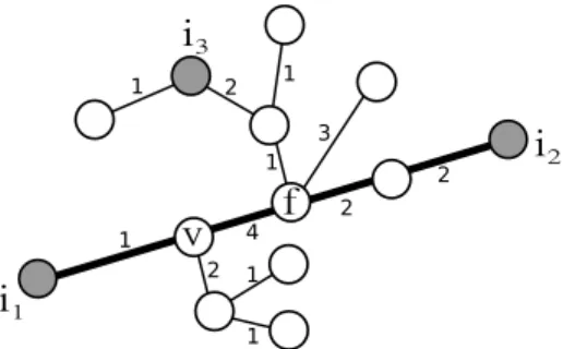
Figure 2 gives a pictorial example of the above concepts.
We now coverMC (the subset of all nodes ofC ∈ C on which SHAZOOmakes a mistake) by the
following subsets:
3
1 2 1 3 2 4 2 1 1 1 2 1
f
v
i
3i
2i
1Figure 2: We illustrate an example of r-node, rn-direction and r-line. The numbers near the edge lines denote edge weights. In order to predictyi2, SHAZOOuses the r-nodei1and the rn-direction
{i1,(i1, v)}. After observingyi2, the hinge line connectingi1withi2(the thick black line) is created,
which is also an r-line, since at the beginning of stept= 2the algorithm used{i1,(i1, v)}. In order
to predictyi3, we still use the r-nodei1and the rn-direction{i1,(i1, v)}. After the revelation ofyi3,
nodefbecomes a fork.
• MF
C is the set of all forks inMC.
• Min
C is the subset ofMCcontaining the nodesiwhose reference nodei∗belongs toC(if
iis a fork, then i∗ = i). Note that this set may have a nonempty intersection with the previous one.
• Mout
C is the subset ofMCcontaining the nodesisuch thati∗does not belong toC.
Two other structures that are relevant to the proof: • CFis the subset of all forksf ∈V
Csuch that∆(f)≤0at some stept. Since we assume
the cluster label is+1(see below), and since a forkit∈VCis mistaken only if∆(it)≤0,
we haveMF C ⊆CF.
• CF0is the subset of all nodes inM
Cthat, when revealed, create a fork that belongs toCF.
Since at each time step at most one new fork can be created,4we have|CF0| ≤ |CF|.
The proof of the theorem relies on the following sequence of lemmas that show how to bound the number of mistakes made on a given clusterC= (VC, EC). A major source of technical difficulties,
that makes this analysis different and more complex than those of TREEOPTandWTA, is that on a weighted tree the value of∆(i)on forksican potentially change after each prediction.
Without loss of generality, from now on we assume all nodes inC are labeled+1. Keeping this assumption in mind is crucial to understand the arguments that follow.
For any nodei∈VC, let∆(i)be the value of∆(i)when all nodes inC\Care revealed.
Lemma 3 For any forkf ofCand any stept= 1, . . . , n, we have∆(f)≤∆(f).
Proof. For the sake of contradiction, assume∆(f)>∆(f). LetTf be the maximal subtree ofT
rooted atf such that no internal node ofTf is revealed. Now, consider the cut given by the edges
ofECφ belonging to the hinge lines ofTf. This cut separatesffrom any revealed node labeled with
−1. The size of this cut cannot be larger thanΦW
C. By definition of∆(·), this implies∆(f)≤Φ W C.
However, also∆(f)cannot be larger thanΦW
C. Because ∆(it)≤ X (i,j)∈Eφ C Wi,j = ΦWC 4
In stepta new forkjis created when the number of edge-disjoint paths connectingjto the labeled nodes increases. This event occurs only when a new hinge lineπ(it, f)is created. When this happens, the only node
for which the number of edge-disjoint paths connecting it to labeled nodes gets increased is the terminal node
must hold independent of the set of nodes inVCthat are revealed before timet, this entails a
contra-diction.
Let nowξCbe the restriction ofξon the subtreeC, and letDCbe the set of all distinct rn-directions
which the nodes ofMin
C can be associated with. The next lemmas are aimed at bounding|CF|and
|DC|. We first need to introduce the supersetD0CofDC. Then, we show that for anyCboth|D0C|
and|CF|are linear inξ C(Φ
W C).
In order to do so, we need to take into account the fact that the sign of∆for the forks in the cluster can change many times during the prediction process. This can be done via Lemma 3, which shows that when all labels inC\Care revealed then, for all forkf ∈C, the value∆(f)does not increase. Thus, we get the largest setDC when we assume that the nodes inC\Care revealed before the
nodes ofC.
Given any clusterC, letσCbe the order in which the nodes ofCare revealed. Let alsoσ0
Cbe the
permutation in which all nodes inCare revealed in the same order asσC, and all nodes inC\C
are revealed at the beginning, in any order. Now, given any node revelation orderσC,D0C can be defined by describing the three types of steps involved in its incremental construction supposingσ0C
was the actual node revelation order.
1. After the first|C\C|= ΦCsteps,DC0 contains all node-edge pairs{i,(i, j)}such thatiis a fork and(i, j)is an edge laying on a hinge line ofC. Recall that no node inCis revealed yet.
2. For each step t > 0 when a new fork f is created such that ∆(f) ≤ 0 just after the revelation ofyit, we add toD
0
Cthe three node-edge pairs{f,(f, j)}, where the(f, j)are
the edges contained in the three hinge lines terminating atf.
3. Letsbe any step where: (i) A new hinge lineπ(is, i∗s)is created, (ii) nodei∗s is a fork,
and (iii)∆(i∗s)≤0at times−1. On each such step we add{is∗,(i∗s, j)}toDC0 , forjin
π(is, i∗s).
It is easy to verify that, given any orderingσCfor the node revelation inC, we haveDC⊆D0C. In
fact, given an rn-direction{i,(i, j)} ∈DC, if(i, j)lies along one of the hinge lines that are present
at time0according toσ0
C, then{i,(i, j)}must be included inD
0
Cduring one of the steps of type 2
above, otherwise{i,(i, j)}will be included inDC0 during one of the steps of type 2 or type 3. As announced, the following lemmas show that|D0
C|and|C
F|are both of the order ofξ C(Φ
W C).
Lemma 4 (i) The total number of forks at timet = ΦC isO ξ(ΦW C)
. (ii) The total number of elements added toD0Cin the first step of its construction isO ξ(ΦW
C)
.
Proof.Assume nodes are revealed according toσ0C. LetC0be the subtree ofCmade up of all nodes inCthat are included in any path connecting two nodes ofC\C. By their very definition, the forks at timet = ΦCare the nodes ofVC0 having degree larger than two in subtreeC0. ConsiderC0 as rooted at an arbitrary node ofC\C. The number of the leaves ofC0is equal to|C\C| −1. This is in turnO ξC(ΦW C because X (i,j)∈Eφ C wi,j =O ξC(Φ W C) .
Now, in any tree, the sum of the degrees of nodes having degree larger than two cannot is at most linear in the number of leaves. Hence, at time t = ΦC both the number of forks inC and the cardinality ofDC0 areO ξC(ΦW
C)
.
Let nowΓT
t be the minimal cutsize ofT consistent with the labels seen before stept+ 1, and notice
thatΓT
Lemma 5 Lettbe a step when a new hinge lineπ(it, q)is created such thatit, q∈VC. If just after
steptwe have∆(q)≤0, thenΓTt −ΓTt−1≥wu,v, where(u, v)is the lightest edge onπ(it, q).
Proof. Since∆(q) ≤ 0andπ(it, q)is completely included inC, we must have∆(q) ≤ 0just
before the revelation ofyit. This implies that the differenceΓ
T t −Γ
T
t−1cannot be smaller than the
minimum cutsize that would be created onπ(it, q)by assigning label−1to nodeq.
Lemma 6 Assume nodes are revealed according toσ0
C. Then the cardinality ofC
F and the total
number of elements added toD0Cduring the steps of type 2 above are both linear inξC(ΦW C).
Proof. LetCF
0 be the set of forks inVC such that∆(f)≤ 0at some timet ≤ |V|. Recall that,
by definition, for each forkf ∈CF there exists a steptf such that∆(f) ≤0. Hence, Lemma 3
implies that, at the same steptf, for each forkf ∈CF we have∆(f)≤0. SinceCF is included in
CF
0, we can bound|CF|by|C0F|, i.e., by the number of forksi∈VCsuch that∆(i)≤0, under the
assumption thatσ0Cis the actual revelation order for the nodes inC. Now,|CF
0|is bounded by the number of forks created in the first|C\C|= ΦCsteps, which is equal
toO ξ(ΦWC)plus the number of forksf created at some later step and such that∆(f)≤0right after their creation. Since nodes inCare revealed according toσ0
C, the condition∆(f) >0just
after the creation of a forkf implies that we will never have∆(f)≤0in later stages. Hence this forkfbelongs neither toC0F nor toCF.
In order to conclude the proof, it suffices to bound from above the number of elements added toD0C
in the steps of type 2 above. From Lemma 5, we can see that for each forkf created at timetsuch that∆(f)≤0just after the revelation of nodeit, we must have|ΓTt −ΓTt−1| ≥wu,v, where(u, v)is
the lightest edge inπ(it, f). Hence, we can injectively associate each element ofCF with an edge
ofEC, in such a way that the sum of the weights of these edges is bounded byΦWC. By definition
ofξ, we can therefore conclude that the total number of elements added toDC0 in the steps of type 2 isO ξ(ΦW
C)
.
With the following lemma we bound the number of nodes of MCin\ CF0 associated with every rn-direction and show that one can perform a transformation of the r-lines so as to make them edge-disjoint. This transformation is crucial for finding the setLT appearing in the theorem statement.
Observe that, by definition of r-line, we cannot have two r-lines such that each of them includes only one terminal node of the other. Thus, let nowFC be the forest where each node is associated
with an r-line and where the parent-child relationship expresses that (i) the parent r-line contains a terminal node of the child r-line, together with (ii) the parent r-line and the child r-line are not edge-disjoint.FCis, in fact, a forest of r-lines. We now usemL(j,v)for bounding the number of mistakes
associated with a given rn-direction{i,(j, v)}or with a givenφ-edge(j, v). Given any connected componentT0ofFC, let finallymT0be the total number of nodes ofMCin\CF
0
associated with the rn-directions{i,(i, j)}of all r-linesL(i, j)ofT0.
Lemma 7 LetCbe any cluster. Then:
(i) The number of nodes inMCin\CF0associated with a given rn-direction{j,(j, v)}is of the order ofmL(i,j).
(ii) The number of nodes inMout
C \C
F0associated with a givenφ-edge(u, q)is of the order
ofmL(u,q).
(iii) LetL(jr, vr)be the r-line associated with the root of any connected componentT0ofFC.
mT0must be at most of the same order of
X
L(j,v)∈L(L(jr,vr))
mL(j,v)+|VT0|
where L(L(jr, vr)) is a set of |VT0| edge-disjoint line graphs completely contained in
Proof. We will prove only (i) and (iii), (ii) being similar to (i). Letit be a node inMCin\C F0
associated with a given rn-direction{j,(j, v)}. There are two possibilities: (a)itis inL(j, v)or (b)
the revelation ofyit creates a forkf inL(j, v)such that∆(f) >0 for all stepss ≥ t. Let now
it0 be the next node (in chronological order) ofMCin\CF 0
associated with{j,(j, v)}. The length ofπ(it0, it)cannot be smaller than the length ofπ(it0, j)(under condition (a)) or smaller than the length ofπ(f, j)(under condition (b)).
This clearly entails a dichotomic behaviour in the sequence of mistaken nodes inMCin\CF0 associ-ated with{j,(j, v)}. Let nowpbe the node inL(j, v)which is farthest fromj such that the length ofπ(p, j)is not larger thanΦW. Once a node inπ(p, j)is revealed or becomes a forkf satisfying ∆(f)>0for all stepss≥t, we have∆(j)>0for all subsequent steps (otherwise, this would con-tradict the fact that the total cutsize ofT isΦW). Combined with the above sequential dichotomic
behavior, this shows that the number of nodes ofMin
C \C
F0 associated with a given rn-direction
{j,(j, v)}can be at most of the order of min ( |L(j, v)|,1 + $ log2 RW L(j,v)+ (Φ W)−1 (ΦW)−1 !%) =mL(j,v).
Part (iii) of the statement can be now proved in the following way. Suppose now that an r-line
L(j, v), havingjandj0as terminal nodes, includes the terminal nodej0of another r-lineL(j0, v0),
havingj0andj00 as terminal nodes. Assume also that the two r-lines are not edge-disjoint. IfL(j0, v0)
is partially included inL(j, v), i.e., ifj00 does not belong toL(j, v), thenL(j0, v0)can be broken into two sub-lines: the first one hasj0andkas terminal nodes, beingkthe node inL(j, v)which is
farthest fromj0; the second one haskandj00 as terminal nodes. It is easy to see thatL(j, v)must be created beforeL(j0, v0)andj0is the only node of the second sub-line that can be associated with
the rn-direction{j0,(j0, v0)}. This observation reduces the problem to considering that inT0 each r-line that is not a root is completely included in its parent.
Given an r-lineL(u, q)havinguandzas terminals, we denote bymπ(u,z)the quantitymL(u,q).
Consider now the simplest case in whichT0is formed by only two r-lines: the parent r-lineL(jp, vp),
which completely contains the child r-lineL(jc, vc). Letsbe the step in which the first nodeuof
L(jp, vp)becomes a hinge node. After step s, L(jp, vp)can be vieved as broken in two
edge-disjoint sublines having{jp, u}and{j0, u}as terminal node sets, wherej0is one of the terminal of L(jp, vp). Thus,
mT0 ≤ max
u∈VL(jp,vp)
mπ(jp,u)+mπ(u,j0)+ 1.
Generalizing this argument for every componentT0ofFC, and using the above observation about
the partially included r-lines, we can state that, for any componentT0ofFC,mT0 is of the order of
max u1,...,uN∈VL(jp,vp) mπ(jp,u1)+mπ(uN,j0)+ N−1 X k=1 mπ(uk,uk+1)+ 2|VT0|
where N = |VT0| − 1. This entails that we can define L(L(jr, vr)) as the union of {π(jp, u1), π(uN, j0)}andS
N−1
k=1 π(uk, uk+1), which concludes the proof.
Lemma 8 The total number of elements added toD0Cduring steps of type 3 above is of the order of
ξC(ΦW C).
Proof.Assume nodes are revealed according toσ0
C, and letsbe any type-3 step when a new element
is added toD0
C. There are two cases: (a)∆(i∗s)≤0at timesor (b)∆(i∗s)>0at times.
Case (a). Lemma 5 combined with the fact that all hinge-lines created are edge-disjoint, ensures that we can injectively associate each of these added elements with an edge ofECin such a way that the
total weight of these edges is bounded byΦW
C. This in turn implies that the total number of elements
added toECisO ξC(Φ W C)
.
Case (b). Since we assumed that nodes are revealed according toσ0
C, we have that∆(i
∗
s)is positive
for all stepst > s. Hence we have that case (b) can occur only once for each of such forksi∗
Since this kind of fork belongs toCF, we can use Lemma 6 and conclude that (b) can occur at most
|CF|=O ξC(ΦW
C)
times.
Lemma 9 With the notation introduced so far, we have|DC|=O ξC(ΦWC).
Proof. Combining Lemma 4, Lemma 6, and Lemma 8 we immediately haveD0C =O ξC(ΦW C)
.
The claim then follows fromDC⊆D0C.
We are now ready to prove the theorem.
Proof of Theorem 2.LetFT be the union ofFCoverC∈ C. Using Lemma 9 we deduce|VFC|= ΦC+O ξC(ΦW C) =O ξC(ΦW C)
, where the termΦC takes into account that at most one r-line ofFCmay be associated with eachφ-edge ofC.
By definition ofξ(·), this implies|VFT|=O ξ(Φ
W)
. Using part (i) and (ii) of Lemma 7 we have |MT| ≤ |MCF|+|M in C|+|M out C | ≤ |C F|+|CF0|+P L∈VFT mL≤PL∈VFT mL+O ξ(ΦW) . Let now T(FT)be the set of components ofFT. Given any treeT0 ∈ T(FT), let r(T0)be the
r-line root ofT0. Recall that, by part (iii) of Lemma 7 for any treeT0 ∈ T(FT)we can find a set
L(r(T0))of|VT0|edge-disjoint line graphs all included inr(T0)such thatmT0 is of the order of
P
L∈LT0(r(T0))mL+|VT0|. Let nowL0T be equal to∪T0∈T(F
T)L(r(T 0)). Thus we have |MT|=O X L∈L0 T mL+|VFT|+ξ(Φ W) =O X L∈L0 T mL+ξ(ΦW) . Observe that L0
T is not an edge disjoint set of line graphs included in T only because each φ
-edge may belong to two different lines of L0
T. By definition of mL, for any line graphs Land
L0, whereL0 is obtained fromLby removing one of the two terminal nodes and the edge incident to it, we have mL0 = mL +O(1). If, for each φ-edge shared by two line graphs of L0T, we shorten the two line graphs so as no one of them includes the φ-edge, we obtain a new set of edge-disjoint line graphsLT such thatPL∈L0
TmL =
P
L0∈L T +ξ(Φ
W). Hence, we finally obtain
|MT|=O P L0∈L TmL 0 +ξ(ΦW) =OP L0∈L T mL 0
, where in the last equality we used the