Improving cluster analysis with automatic variable selection based on trees

Calhoun: The NPS Institutional Archive

Theses and Dissertations Thesis Collection

2014-12

Improving cluster analysis with automatic variable

selection based on trees

Orr, Anton D.

Monterey, California: Naval Postgraduate School

NAVAL

POSTGRADUATE

SCHOOL

MONTEREY, CALIFORNIA

THESIS

Approved for public release; distribution is unlimited IMPROVING CLUSTER ANALYSIS WITH AUTOMATIC

VARIABLE SELECTION BASED ON TREES

by Anton D. Orr December 2014

Thesis Advisor: Samuel E. Buttrey Second Reader: Lyn R. Whitaker

REPORT DOCUMENTATION PAGE _{Form Approved OMB No. 0704–0188}

Public reporting burden for this collection of information is estimated to average 1 hour per response, including the time for reviewing instruction, searching existing data sources, gathering and maintaining the data needed, and completing and reviewing the collection of information. Send comments regarding this burden estimate or any other aspect of this collection of information, including suggestions for reducing this burden, to Washington headquarters Services, Directorate for Information Operations and Reports, 1215 Jefferson Davis Highway, Suite 1204, Arlington, VA 22202-4302, and to the Office of Management and Budget, Paperwork Reduction Project (0704-0188) Washington, DC 20503.

1. AGENCY USE ONLY (Leave blank) 2. REPORT DATE December 2014

3. REPORT TYPE AND DATES COVERED Master’s Thesis

4. TITLE AND SUBTITLE

IMPROVING CLUSTER ANALYSIS WITH AUTOMATIC VARIABLE SELECTION BASED ON TREES

5. FUNDING NUMBERS

6. AUTHOR(S) Anton D. Orr

7. PERFORMING ORGANIZATION NAME(S) AND ADDRESS(ES) Naval Postgraduate School

Monterey, CA 93943-5000

8. PERFORMING ORGANIZATION REPORT NUMBER

9. SPONSORING /MONITORING AGENCY NAME(S) AND ADDRESS(ES) N/A

10. SPONSORING/MONITORING AGENCY REPORT NUMBER

11. SUPPLEMENTARY NOTES The views expressed in this thesis are those of the author and do not reflect the official policy or position of the Department of Defense or the U.S. Government. IRB Protocol number ____N/A____. 12a. DISTRIBUTION / AVAILABILITY STATEMENT

Approved for public release; distribution is unlimited

12b. DISTRIBUTION CODE A

13. ABSTRACT (maximum 200 words)

Clustering is an algorithmic technique that aims to group similar objects together in order to give users better understanding of the underlying structure of their data. It can be thought of as a two-step process. The first step is to measure the distances among the objects to determine how dissimilar they are. The second, clustering, step takes the dissimilarity measurements and assigns each object to a cluster.

We examine three distance measures proposed by Buttrey at the Joint Statistical Meeting in Seattle, August 2006 based on classification and regression trees to address problems with determining dissimilarity. Current algorithms do not simultaneously address the issues of automatic variable selection, independence from variable scaling, resistance to monotonic transformation and datasets of mixed variable types.

These "tree distances" are compared with an existing dissimilarity algorithm and two newer methods using four well-known datasets. These datasets contain numeric, categorical and mixed variable types. In addition, noise variables are added to test the ability of each algorithm to automatically select important variables. The tree distances offer much improvement for the problems they aimed to address, performing well against competitors amongst numerical datasets, and outperforming in the cases of categorical and mixed variable type datasets.

14. SUBJECT TERMS Clustering, Classification Trees, Regression Trees, Random Forests, Sparse Hierarchical, Sparse K-means

15. NUMBER OF PAGES 61 16. PRICE CODE 17. SECURITY CLASSIFICATION OF REPORT Unclassified 18. SECURITY CLASSIFICATION OF THIS PAGE Unclassified 19. SECURITY CLASSIFICATION OF ABSTRACT Unclassified 20. LIMITATION OF ABSTRACT UU

Approved for public release; distribution is unlimited IMPROVING CLUSTER ANALYSIS WITH AUTOMATIC VARIABLE

SELECTION BASED ON TREES

Anton D. Orr

Commander, United States Navy B.S., United States Naval Academy, 1995

Submitted in partial fulfillment of the requirements for the degree of

MASTER OF SCIENCE IN OPERATIONS RESEARCH

from the

NAVAL POSTGRADUATE SCHOOL December 2014

Author: Anton D. Orr

Approved by: Samuel E. Buttrey Thesis Advisor

Lyn R. Whitaker Second Reader

Robert F. Dell

ABSTRACT

Clustering is an algorithmic technique that aims to group similar objects together in order to give users better understanding of the underlying structure of their data. It can be thought of as a two-step process. The first step is to measure the distances among the objects to determine how dissimilar they are. The second clustering step takes the dissimilarity measurements and assigns each object to a cluster.

We examine three distance measures proposed by Buttrey at the Joint Statistical Meeting in Seattle, August 2006 based on classification and regression trees to address problems with determining dissimilarity. Current algorithms do not simultaneously address the issues of automatic variable selection, independence from variable scaling, resistance to monotonic transformation and datasets of mixed variable types.

These “tree distances” are compared with an existing dissimilarity algorithm and two newer methods using four well-known datasets. These datasets contain numeric, categorical and mixed variable types. In addition, noise variables are added to test the ability of each algorithm to automatically select important variables. The tree distances offer much improvement for the problems they aimed to address, performing well against competitors amongst numerical datasets, and outperforming in the cases of categorical and mixed variable type datasets.

TABLE OF CONTENTS

I. INTRODUCTION ... 1

II. BACKGROUND AND LITERATURE REVIEW ... 5

A. DISSIMILARITY MEASUREMENTS FOR NUMERIC VARIABLES .... 6

1. Euclidean and Manhattan Distance ... 6

2. Variable Weights ... 8

B. DISSIMILARITY MEASUREMENTS FOR MIXED VARIABLES ... 10

1. Binary Variables ... 10

2. General Categorical Variables ... 12

3. Mixed Variables ... 13

C. CLASSIFICATION AND REGRESSION TREES ... 14

1. Regression Trees ... 14

2. Classification Trees ... 15

3. Random Forest Distance... 16

D. CLUSTERING ALGORITHMS ... 18 1. Partitioning Algorithms ... 18 a. K-means ... 18 b. PAM ... 19 2. Hierarchical Algorithms ... 19 3. Sparse Clustering ... 20 a. Sparse K-means ... 20 b. Sparse Hierarchical... 20 III. METHODOLOGY ... 23 A. INTRODUCTION ... 23

B. BUTTREY TREE DISTANCES ... 23

1. Tree Distance 1, d1 ... 24

2. Tree Distance 2, d2 ... 24

3. Tree Distance 3, d3 ... 25

C. ALGORITHMS USED ... 26

D. EVALUATION USING CRAMÉR’S V ... 27

E. DATASETS ... 27 1. Iris ... 28 2. Optical ... 29 3. Splice ... 29 4. Cardiac Arrhythmia ... 29 IV. ANALYSIS ... 31 A. INTRODUCTION ... 31 B. RESULTS ... 31 C. CONCLUSION ... 34

B. FUTURE WORK... 35 LIST OF REFERENCES ... 37 INITIAL DISTRIBUTION LIST ... 39

LIST OF FIGURES

Figure 1.   Illustration of Euclidean distance. ... 7  

Figure 2.   Illustration of Manhattan distance. ... 8  

Figure 3.   Tree with deviance in large circles and leaf numbers in small circles (from Buttrey, 2006) ... 25  

Figure 4.   Example tree evaluated using d3 with deviances for leaf 14 and 15 (from Lynch, 2014) ... 26  

LIST OF TABLES

Table 1.   Observation i and j association table ... 10  

Table 2.   Dimensions of datasets ... 28  

Table 3.   Iris Dataset Results ... 32  

Table 4.   Optical Digits Dataset Results ... 33  

Table 5.   Splice Dataset Results ... 33  

LIST OF ACRONYMS AND ABBREVIATIONS

Agnes agglomerative nesting

BCSS between cluster sums of squares CART classification and regression trees Daisy DISsimilAritY

PAM partitioning around medoids PMA penalized multivariate analysis SPC sparse principal components

UPGMA unweighted pair-group average method WCSS within cluster sums of squares

EXECUTIVE SUMMARY

Grouping similar objects together is an instinctual response when trying to organize or process an array of information. This sorting and classification process dates back to Aristotle’s work on biological taxonomy (Hartigan, 1975). Since then, most fields have developed their own processes to accomplish the task, and data scientists use clustering algorithms.

Clustering can be thought of as a two-step process. The first step is the measurement of distance, or more generally, dissimilarity between observations. The second step is assigning each object to a specific group or “cluster.” Our focus is to improve clustering techniques that are applied to the types of data encountered by military practitioners. Often such data consists of a mix of both numeric and categorical data. For example, military manpower studies of promotion rates include numeric variables such as “age” and “number of dependents” as well as categorical variables such as “education level,” “commissioning source” and “marital status” (Kizilkaya, 2004). In addition, it is common that in such studies the number of variables is great, but the number of relevant variables for clustering is small.

The book by Kaufman and Rousseeuw (1990) presents different variable types and ways to measure distance along with the two main clustering methods. Numerical variables can be measured using either Euclidean or Manhattan distance, although both are susceptible to scaling or monotonic transformation. Dissimilarities for categorical and mixed data types can be measured using a generalization of Gower’s (1971) formula. A common practice is to use Euclidean distance when all variables are numeric and Gower dissimilarity for datasets of mixed variable types as is implemented by the daisy function in the R software (R Core Team, 2014) package “cluster” (Maechler, Rousseeuw, Struyf, Hubert, & Hornik, 2014).

Current clustering algorithms do not simultaneously address these key issues:

• Independence from variable scaling • Automatic selection of important variables • Resistance to monotonic transformation

• Inputs with mixed numerical and categorical variables.

A new approach by Buttrey (2006) uses classification and regression trees to define three new distances (tree distances) that attempt to address these issues. This thesis compares these tree distances to dissimilarities computed by daisy and the random forest proximities proposed by Breiman (2001). These five distances are computed for four existing and well-known datasets and input into the clustering algorithms Agnes (agglomerative nesting), PAM (partitioning around medoids) and K-means. Noise is introduced into each dataset to test automatic variable selection. An additional method that uses sparse hierarchical and sparse k-means combines the distance measurement and clustering steps is introduced by Witten and Tibshirani (2010) and is also used for comparison.

The tree distances take a dataset of n observations and p variables and create a classification or regression tree using each variable as the response. After the trees are created, each object is run down the tree. For the first distance d1, two objects are considered similar if they end up in the same leaf. The second distance, d2, scales the dissimilarity of objects by the “quality” of each tree, which is determined by the amount of deviance between the root node and leaves. The third distance, d3, computes dissimilarity between objects by comparing deviance at their parent node to the deviance at the root node.

Of the distance metrics tested, d2 consistently performed well across all four datasets.

LIST OF REFERENCES

Breiman, L. (2001). Random forests. Machine Learning, 45(1), 5–32.

Buttrey, S. E. (2006). A Scale-Independent Clustering Method with Automatic Variable Selection Based on Trees. Joint Statistical Meetings. Seattle, WA.

Gower, J. C. (1971). A general coefficient of similarity and some of its properties. Biometrics, 27(4), 857–871.

Hartigan, J. A. (1975). Clustering algorithms. New York, NY: Wiley.

Kaufman, L., & Rousseeuw, P. (1990). Finding groups in data: An introduction to cluster analysis. New York: John Wiley & Sons, Inc.

Kizilkaya, Z. (2004). An Analysis of the Effect of Commissioning Sources on Retention and Promotion of U.S. Army Officers (Master’s thesis). Retrieved from http://calhoun.nps.edu

Maechler, M., Rousseeuw, P., Struyf, A., Hubert, M., & Hornik, K. (2014). Cluster: Cluster analysis basics and extensions. (R Package Version, 1.15.2)

R Core Team. (2014). R: A language and environment for statistical computing. Vienna, Austria: R Foundation for Statistical Computing.

Witten, D. M., & Tibshirani, R. (2010). A framework for feature selection in clustering. Journal of the American Statistical Association, 105(490), 713– 726.

ACKNOWLEDGMENTS

I would like to thank Professors Samuel Buttrey and Lyn Whitaker for their patience and guidance throughout this process. It is said that nothing worth having is easy, and this program has been no exception. Working with you has made this process almost enjoyable. Your time, enthusiasm, and guidance in helping me navigate this task have been immeasurable.

I would also like to thank my children and family for all the support and sacrifices you’ve made throughout my time in the Navy. I would not have accomplished any of the things I have without it.

I.

INTRODUCTION

Classification dates back to Aristotle’s biological work on the taxonomy of plants and animals. Clustering is the grouping of similar objects and is a counterpart of classification (Hartigan, 1975). Algorithms, whose modern usage has extended into the fields of astronomy, medicine, economics, and many other types of data analysis, implement the more formal technique of clustering. Military and industry practitioners of data analytics face the challenge of turning an abundance of information into useful tools that can assist in making critical decisions. The amount of data collected by private industry and government institutions can be on the order of terabytes daily and clustering techniques can aid the decision-making process by helping to identify and visualize the patterns in this data. Finding the signal in this sea of “noise” will require improvements to the tools we currently use.

Our focus is to improve clustering techniques that are applied to the types of data encountered by military practitioners. Often such data consists of a mix of both numeric and categorical data. For example, military manpower studies of promotion rates include numeric variables such as “age” and “number of dependents” as well as categorical variables such as “education level,” “commissioning source,” and “marital status” (Kizilkaya, 2004). In addition, it is common that in such studies the number of variables is great, but the number of relevant variables for clustering is small. In this thesis, we build on the work of Lynch’s (2014) empirical study of a new and novel clustering technique from Buttrey (2006), specifically designed to cluster observations with mixed categorical and numeric variables and which promises to be robust when applied to datasets with a large number of irrelevant and noisy variables.

Clustering is an algorithmic technique. Which algorithm is used depends on a number of factors including the tradition of the field of application, the types

numeric variables (e.g. Ooi, 2002), although there are notable attempts to treat clustering of categorical variables and mixed variables (e.g. Zhang, Wang and Zhang, 2007). A recent research trend in the area of clustering concerns variable selection, i.e., when confronted with a large (big) data set with many variables, which should be used or weighted more heavily when clustering (e.g. Witten & Tibshirani, 2010). Few works explicitly address both the issues of clustering mixed variables and variable selection.

The process of clustering can be thought of as a two-step process. At the center is the measurement of distance, or more generally, dissimilarity between observations. This aspect of clustering is given much less attention in the literature than the second step (Hastie, Tibshirani and Friedman, 2009). The second step, the clustering step, is the process of grouping like objects into clusters. For clustering based on numeric variables, the choice of dissimilarity measurement is problematic. It depends, among other things, on the choice of an appropriate scale for each variable and on how much weight each variable will be given in the dissimilarity computation. Combining categorical variables with numeric variables complicates the choice of dissimilarity measurement further.

Current clustering algorithms that implicitly or explicitly produce distance calculations do not simultaneously address these key issues:

• Independence from variable scaling • Automatic selection of important variables • Resistance to monotonic transformation

• Inputs with mixed numerical and categorical variables

The fundamental contribution of Buttrey (2006) is his approach to using classification and regression trees to define distances (tree distances) that address each of these four key issues. Lynch (2014) studies three tree distances and shows that clustering based on two of the tree distances is advantageous

clustering. In our work, we explicitly decouple the dissimilarity measuring process from the clustering process. This allows us to include in our study a comparison of tree distances with two competing dissimilarities for mixed variables. By decoupling the dissimilarity computations from the clustering algorithm, we also extend the sparse clustering methods of Witten and Tibshirani (2010) so that they can be used to cluster mixed variable datasets. This allows us to experiment with the use of more modern clustering algorithms that are not explicitly designed for mixed variables.

This thesis examines the ability of five methods for determining dissimilarities amongst observations in datasets with and without mixed variables. Their performance will be evaluated based on the clustering solutions they produce for four existing and well-known datasets. The five dissimilarities include the three new tree distances and two existing dissimilarities: one of Euclidean distance for numeric variables or the ubiquitous Gower (1971) dissimilarity, a generalization of the Gower coefficient, for mixed variables, and the lesser known distance based on Breiman’s (2001) random forest proximities. Each will be matched with at least two clustering algorithms to establish whether the new tree distances produce better results, and if so, what the causes are. In addition, because a benefit of tree distances is their robustness when noisy or irrelevant variables are present, we also produce results for two clustering methods of Witten and Tibshirani (2010). Their sparse clustering incorporates variable selection into the distance computations and has been observed to perform well for datasets with few relevant variables.

This paper is organized as follows. Chapter II introduces common dissimilarities for numeric, categorical, and mixed variables and describes distances based on random forest proximities. Chapter II also reviews some of the current clustering methodology. Chapter III is an introduction to the new tree distances and review of the datasets used in the study. Chapter IV presents findings and analysis of the research. Finally, chapter V provides conclusions

II.

BACKGROUND AND LITERATURE REVIEW

There are many approaches to the problem of clustering and many finely detailed aspects addressed in academic texts and papers. Two often referenced sources on which we rely heavily to lay the groundwork for clustering are the books by Kaufman and Rousseeuw (1990) and Hastie, Tibshirani and Friedman (2009). Kaufman and Rousseeuw (1990) cover many of the algorithms used to measure dissimilarity between observations and group them into clusters. The second book by Hastie, Tibshirani and Friedman (2009), covers many of the same techniques as do Kaufman and Rousseeuw (1990) and introduces a unique distance measurement technique that will be examined further in this paper.

The basic idea for clustering is to take a dataset with n observations and p measurements (variables) and separate them into groups, or “clusters,” based on their proximities. Thus, in this chapter, we begin by discussing common methods for measuring proximities starting with numeric variables and then discussing mixed numeric and categorical variables. We then give a review of classification and regression trees (CART). CART forms the basis of the new tree distances introduced in Chapter III. CART is also the basis of a competing distance computed from the Breiman (2001) random forest proximities and described in this chapter.

We note that most clustering algorithms do not require that a distance characterize proximities between observations. Most clustering algorithms will take dissimilarities rather than distances, where the dissimilarities have the following properties: the dissimilarity of an object with itself is zero, all dissimilarities are non-negative, and the dissimilarity between object i and object j is the same as the dissimilarity between object j and object i.

restrictive term dissimilarity to mean either distance or dissimilarity. Further, proximity is the general term which can be measured by how far apart objects are or by closeness or similarity, where similarity is a monotonic decreasing function of dissimilarity (often similarity is one minus dissimilarity).

A. DISSIMILARITY MEASUREMENTS FOR NUMERIC VARIABLES

There are many ways to measure the dissimilarity between objects i and j. Two of the most common for continuous numeric variables are Euclidian distance and Manhattan distance. These are suitable for variables that are positive or negative real numbers on a linear scale, such as age, weight, cost, length, etc. Numeric variables can be subjected to a change in units or monotonic transformations that will affect their distance. For linear forms, the primary way to handle these changes is standardization, so that relative distances between observations remain constant.

1. Euclidean and Manhattan Distance

Euclidean distance is the true geometrical distance between two points i and j with coordinates (xi1,..., xip) and (xj1,…, xjp), and is given by the equation:

d(i,j)= (xi1−xj1) 2₊ (xi2−xj2) 2₊ ...+(xip−xjp) 2 _(2.1) where the x’s are numeric and the number of variables are measured by p (Kaufman and Rousseeuw, 1990). Equation 2.1 gives the length of the hypotenuse of the triangle, so this distance is sometimes referred to as Pythagorean distance and is illustrated in Figure 1.

Figure 1. Illustration of Euclidean distance.

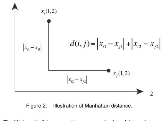
The second well-known distance metric is the Manhattan distance, or city block. This is the distance between two points in a grid based strictly on a horizontal and/or vertical line of travel instead of the diagonal route. This distance is the sum of the absolute value of the difference between each variable:

d(i,j)= xi1−xj1 + xi2−xj2 +...+ xip−xjp (2.2) and is illustrated in Figure 2.

Figure 2. Illustration of Manhattan distance.

The Minkowski distance provides a generalization of these distances d(i,j)=

(

x_i1−x_j1q+ x_i2−x_j2q+...+ x_ip−x_jpq

)

1/q

(2.3)

in which q is any real number greater than or equal to 1 (Kaufman & Rousseeuw, 1990).

The distance algorithm daisy (DISssimilAritY) implemented in the R package (R Core Team, 2014) “cluster” (Maechler, Rousseeuw, Struyf, Hubert, & Hornik, 2014), which will be discussed later and which we use in this study, can use either the Euclidean or Manhattan distance for its calculations when all variables are numeric.

2. Variable Weights

The distances (2.1), (2.2), and (2.3) weigh each variable equally. Other considerations in distance measurements concern the importance of individual variables and their weight towards the calculations. For example, changing the scale of a variable by converting from meters to kilometers would change the

through standardization of the variables. Kaufman and Rousseeuw (1990) accomplish this with three steps. First, calculate the mean for variable f,

m_f =1

n

(

x1f +x2f +...+xnf

)

. (2.4)

Then take the mean absolute deviation s_f =1

n

{

x1f −mf + x2f −mf +...+ xnf −mf

}

. (2.5) Use the mean (2.4) and the mean absolute deviation (2.5) to standardize the variable in a “z-score” calculation

z_if = xif −mf

s_f . (2.6)

Standardization (2.6) gives all variables an equal weight independent of their units (Kaufman & Rousseeuw, 1990). Often practitioners use either the sample standard deviation of the range in place of the mean absolute deviation in (2.5). The advantage of using the mean absolute deviation over the sample standard deviation or the variable range is that it is more robust to extreme values.

More generally, it must be decided if all variables should have equal importance before clustering. Some variables matter more than others and this consideration requires some subject matter expertise. A hypothetical dataset of aircraft might include age, top speed, gross weight, empty weight, cost and tail number. If you wanted to cluster the aircraft according to cargo-carrying capability, gross weight might be a better discriminant than age, and should be weighted appropriately. Tail number probably provides no useful information, so it might be excluded or equivalently given a weight of 0. Weighted Euclidian distance is given by d(i,j)= w₁(x_i1−x_j1)2+_w 2(xi2−xj2) 2+_...+_w p(xip−xjp) 2 _(2.7)

where w is the weight applied to each variable, and can be used to indicate perceived importance (Kaufman & Rousseeuw, 1990). Both Kaufman and Rousseeuw (1990) and Hastie, Tibshirani and Friedman (2009) see this process

current work (Witten and Tibshirani, 2010) seeks to automate this process through variable selection, which computes the variable weight, with selected (irrelevant) variables getting weight zero.

B. DISSIMILARITY MEASUREMENTS FOR MIXED VARIABLES

Different types of variables require different approaches when considering their proximities for clustering. For non-numeric variables, we start by considering dissimilarities based only on categorical variables with two levels each (binary variables). We then discuss dissimilarities between nominal and ordinal categorical variables with two or more levels and then show the most common approach to combining numeric and categorical variables.

1. Binary Variables

Categorical variables with two levels are common in practice. For example, an attribute can be present/absent, yes/no, male/female, or small/large. Often such variables are encoded as binary 0/1 variables. When these characterizations are symmetric, of equal value, similar weight, and all variables in a dataset are binary, the similarity between two observations is calculated with a matching coefficient derived from an association table:

Table 1. Observation i and j association table object j

1 0

object i 1 a b a+b

0 c d c+d

a+c b+d

In Table 1, the value depicted by a is the sum of binary attributes where object i and object j both equal 1 and d is where they both equal 0. The matching

s(i,j)= a+d

a+b+c+d , (2.8) where the numerator is the total number of matches and the denominator, the total number of binary variables (Kaufman & Rousseeuw, 1990).

The corresponding dissimilarity would be d(i,j)=1−s(i,j), with coefficients taking on values from 0 to 1. The algorithm daisy default is to use this coefficient to compute dissimilarities between observations when all variables are binary categorical variables.

Another type of binary variable is asymmetric. One value, usually taken to be 1, of an asymmetric binary variable is rare, so most objects would have a value of 0. When compared for similarity, negative matches would be expected, so positive matches are considered more significant.

An example dataset of aircraft might include a variable of aircraft type, measuring whether the aircraft is an attack aircraft, with value 1, or not, with value 0. In this case, for variable f corresponding to aircraft type the statement xif = 1 and xjf = 1 is a rare positive match, and implies that aircraft i and j are both attack aircraft. In this dataset of civilian aircraft, a negative match “non-attack,” is common and less meaningful because the two could be of many different aircraft types. To calculate similarities, only positive matches are considered, where sijf = 1 for each match at variable f, giving similarity between aircraft i and j

sijf f=1

p

∑

p . (2.9)

To accommodate missing values, let sijf = 1 if variable f can be measured for both object i and j and define the similarity to be

s(i,j)= δijfsijf f=1 p

∑

δijf f=1 p

∑

. (2.10)

This is Gower’s (1971) general similarity coefficient for asymmetric binary categorical variables, and can be implemented in daisy.

2. General Categorical Variables

The last variable type is categorical. This variable comes in the form of nominal or ordinal values. Nominal variable types are for observations that take on multiple values, where the values are not ranked and are simply labels. Ordinal values have a ranking attached.

An example of a nominal categorical variable would be the county in which a person resides, with the counties encoded by values one through five. When measuring dissimilarity, the difference between counties one and two should be the same as to the difference between counties two and five. The most common way to calculate dissimilarity for a nominal categorical variable f is a simple matching approach: d_ijf = 0 if xif =xjf 1 if x_if ≠x_jf ⎧ ⎨ ⎪ ⎩⎪ . (2.11)

When all p variables are nominal categorical variables the dissimilarity is calculated as the average of individual dissimilarities that are available for both objects i and j: d(i,j)= δijfdijf f=1 p

∑

δijf f=1 p

∑

. (2.12)

Ordinal variables take on different states like nominal values, except they have a meaningful order. An example would be responses to survey questions with values one through five on a five point Likert scale. The states range from strongly disagree = 1, to strongly agree = 5, and the difference between states 1 and 2 would not be equivalent to the difference between 2 and 5.

scoring is to base the scores on the ranks of the observations. For example, if the ordered states are 1, 2,..., M, a z-score can be created using the rank rif of the i-th observation in the f-th variable by

z_if = rif −1

M_f −1 (2.13)

where Mf is the highest state for variable f. The z-score will take on values 0 to 1. When all p variables are ordinal, the dissimilarity between observations i and j can then be calculated by the Manhattan distance divided by the number of variables being considered (Kaufman & Rousseeuw, 1990).

3. Mixed Variables

So far, we are able to compute distances for five variable types: numeric, symmetric and asymmetric binary, and nominal and ordinal categorical. When different types occur in the same dataset, we need a way to combine them. In this section we describe Gower’s approach to computing dissimilarities for mixed variables. This approach is implemented by daisy as the default for datasets with mixed variables.

First, the dissimilarity for each variable is scaled to be between 0 and 1, i.e., for any pair of objects i, j the dissimilarity for variable f = 1, .., p is 0≤dijf ≤1.

Once these calculations have been made, an overall dissimilarity can be defined for datasets that contain p variables of a mixed nature

d(i,j)= f=1δijfdijf

p

∑

δijf f=1 p

∑

, (2.14)

where, as before, δijf is equal to 1 when both xif and xjf for the f-th variable are

non-missing (Kaufman & Rousseeuw, 1990).

In (2.14) d_ijf is the contribution of the f-th variable to the dissimilarity between i and j. If either observation is missing on variable f, δijf= 0 and that

(2.10) gives the dissimilarity. For continuous or ordinal variables, the dissimilarity is given by

dijf =

xif −xjf

R_f (2.15)

where Rf is the range of variable f,

R_f =max

h xhf −minh xhf (2.16)

and h covers all non-missing observations for variable f.

C. CLASSIFICATION AND REGRESSION TREES

When dealing with datasets that involve a large number of variables, classification and regression trees (CART) are often used (Breiman, Friedman, Stone, & Olshen, 1984). These are simple nonlinear predictive models that recursively partition a data space and fit a decision tree into each partition. Regression trees are used when the response variable has continuous values, and classification trees when a response has a finite number of unordered values or “classes.”

1. Regression _Trees

Regression tree algorithms take an observation with a numeric response y and p input variables for each of n observations: that is (y_i|x_i) for i = 1, 2, ...,n, with input variables xi=(xi1,xi2,...,xip) (Hastie, Tibshirani, & Friedman, 2009). The algorithm automatically decides the splitting variable and split to produce a partition with M regions R1, R2, ..., RM. For each region, the predicted response,

y(x) is modeled as a constant cm, so that

y(x)= c_mI(x∈R_m)

m=1 M

∑

(2.17)

where I(x∈Rm) is the indicator function which is 1 is x∈Rm and 0 otherwise.

ˆ

cm=ave(yi|xi∈Rm) . (2.18) A tree is grown starting with the root node, which contains all observations. Proceeding with a greedy algorithm, at each node R, a splitting variable j and split point s (or set s for categorical variables) will partition the node R into left and right child nodes defined by

RL(j,s)=

{

xij∈R|xij ≤s

}

and RR(j,s)=

{

xij∈R|xij>s

}

(2.19) for numeric variables xj. For categorical variables,

R_L(j,s)=

{

x_ij∈R|x_ij∈s

}

and R_R(j,s)=

{

x_ij ∈R|x_ij∈s

}

(2.20) where s is a subset of the levels of the categorical variable.

The values for j, s and c_L, c_{R, the predicted values for} y in the left and right child nodes respectively are found by solving

min j,s mincL (yi−cL) 2 xij∈RL(j,s)

∑

+min cR (yi−cR) 2 xij∈RR(j,s)

∑

⎡ ⎣ ⎢ ⎢ ⎤ ⎦ ⎥ ⎥ , (2.21)

the combined “impurity” of the two child nodes (Hastie, Tibshirani, & Friedman, 2009).

For each splitting variable j and split s, the inner minimization is solved by ˆ

c_L=ave y

(

_i|x_i∈R_L(j,s)

)

and ˆc_R =ave y

(

_i|x_i∈R_R(j,s)

)

(2.22) This algorithm will grow a tree and stops when a node size limit or a threshold value for equation (2.21) is reached. This tends to produce a tree which is too large. With large trees there is a danger of over-fitting. That is, the tree is grown to a depth that predicts each observation in the data set well, but it cannot predict observations taken from an independent, but similar data set. To guard against over-fitting, the tree is then “pruned” by collapsing internal nodes to find a subtree that minimizes ten-fold cross-validated measure of impurity.

2. Classification Trees

main difference being the criteria used to split nodes. The proportion of objects in node m, which represents region Rm and nm observations is shown by,

ˆ p_mk = 1 nm I(y_i =k) xi∈Rm

∑

(2.23)

where k is the class. The majority of observations residing in node m determine its classification: k(m)=arg maxk ˆpmk. At each split, a variable and splitting criteria are chosen to minimize the impurity of the child nodes. A common measure of impurity and the one we use is the multinomial deviance,

−2 _i=1nmklog( K

∑

pˆmk)_. (2.24)

As with regression trees, classification trees are pruned so that the ten-fold cross-validated deviance is minimized.

3. Random Forest Distance

The random forest concept was introduced by Breiman (2001) and builds multiple classification or regression trees to reduce variance, creating a “forest” of trees. In addition to prediction, Breiman (2003) discuses a number of applications of random forests including the notion of using random forests to measure the proximity between two observations. In this thesis, random forests are used to measure dissimilarities between two observations based on Breiman’s proximities.

The steps for building a random forest based on a dataset with n observations are:

For b = 1 to B:

1. Draw n cases at random, with replacement, from the dataset to create a training set. This training set is called a “bootstrapped” sample.

2. Grow tree Tb using the bootstrapped sample by repeating the following steps at each node, until a minimum node size nmin is reached:

a) Select m << p variables at random from the original variables. (typically m= p)

b) Pick the best variable and split among m. c) Split the node into two child nodes.

The output is the set of trees

{ }

T_{b 1}B.

For a categorical response, the class prediction of the b-th random forest tree will be _Cˆ

b(x), making the final prediction Cˆrf

B_(x)=_{majority vote ˆC} b(x)

{ }

1

B

(Hastie, Tibshirani, & Friedman, 2009). For a numeric response, y_b(x) is the prediction for the b-th random forest tree and the final prediction is the forest average.

Breiman (2001) uses random forests to measure proximity between observations. In this setting there is no response variable. His solution is to label all n observations in the dataset to have value y=1 and then to simulate “observations” for the y=0 class. The y=0 observations are generated so that their marginal distributions match the marginal distributions of the original data, but so that the variables of the simulated observations are independent. Building random forests to correctly classify the combined data can uncover structural properties, like clusters, of the original y=1 observations, which are not present in the simulated y=0 observations. Breiman calls this method unsupervised random forests.

After each tree in the random forest is built, all the observations are run down each tree and if two (i and j) end up in the same leaf, their similarity s(i,j)

is increased by one. After all similarities are totaled, they are normalized by dividing by the number of trees. This is used to create a distance between any two observations d(i,j)=1−s(i,j); i.e., the distance between observations i and j

D. CLUSTERING ALGORITHMS

There are two primary families of clustering methods, implemented by either partitioning or hierarchical algorithms (a third approach, model based clustering, is not discussed here). They both require a dissimilarity matrix as the input. A dissimilarity matrix for n observations is the n x n matrix of dissimilarities or distances

{

d(i,j)

}

nxn. The two types of clustering methods (partitioning and hierarchical methods) are often used for comparison to see which produces a better cluster organization.

1. Partitioning Algorithms

Partitioning algorithms take all n observations and group them into K clusters. The user inputs the value for K, so it is advisable to try different values for K to see which output produces the best result. There are many algorithms, but this thesis will discuss the two most popular, K-means and PAM.

a. K-means

Given a set of multivariate observations (x1, x2, ... ,xn), K-means partitions the n observations into K clusters C=

{

C₁,C₂,...,C_K

}

so as to minimize the

within-cluster sum of squares (WCSS). The objective is to find:

arg min C x−µ_k 2 x∈Ck

∑

k=1 K

∑

(2.25)

where µk is the mean of observations in Ck (MacQueen, 1967).

The algorithm proceeds in two steps. First, an initial set of K means m1, ...,

mK is chosen at random and each observation is assigned to the cluster that is

closest. After all observations have been assigned, the centroid of each cluster becomes the new mean. The process starts again by reassigning observations to the new means until convergence and the assignments stop changing. This does not guarantee a global optimum, so the algorithm can be run multiple times with

K-means uses Euclidean distance in (2.25) to measure the distance from observations in a cluster to the cluster center. In addition, a cluster center is the average of the observations in that cluster. For these two reasons, K-means can only be used when all variables are numeric and Euclidean distance is appropriate.

b. PAM

Partitioning around medoids uses the K-medoids algorithm which is related to K-means. They both attempt to minimize squared error, with the difference being that PAM always chooses a datapoint as the center of a cluster instead of using the centroid of i-th cluster. This algorithm can be more robust to noise and outliers than K-means. Further, PAM can be adapted to handle datasets with mixed variable types. Using the medoid as the cluster center requires no averaging of observations and because a cluster medoid is one of the observations in the dataset, dissimilarity between it and the members of the cluster can be measured by any dissimilarity or distance defined for mixed variables.

2. Hierarchical Algorithms

Hierarchical algorithms do not construct a single partition with K clusters, but offer all combinations of clusters from K = 1 (all observations in one cluster) to K = n (each observation in its own cluster). This paper will address the agglomerative nesting (Agnes) technique that starts with K = n.

This method begins by joining the two observations that are closest together, leaving n − 1 clusters. Once the first cluster is created, for subsequent pairings, the distances are measured using the unweighted pair-group average method (UPGMA). This method measures dissimilarities between all objects in two clusters and takes the average value. This process is continued until K = 1. Different techniques are then applied to determine the optimal number of clusters

observations in the dataset. However, it requires that all n(n−1)

2 pairwise dissimilarities be computed, a computational load that can be burdensome for large datasets.

3. Sparse Clustering

Clustering data with a large set of p variables introduces the challenge of selecting which ones actually differentiate the observations. Witten, Tibshirani and Hastie (2010) present a method of sparse K-means and sparse hierarchical clustering that address this problem. These two new methods will be used with the two previously described traditional clustering algorithms for this paper’s analysis.

a. Sparse K-means

The sparse K-means algorithm operates by maximizing the between-cluster (weighted) sum of squares (BCSS), which is the equivalent to K-means minimization of WCSS. A weight w1,..., wp, is assigned to each of the p variables. The value of ||w|| ≤ s, where w = (w1,..., wp) and s is a tuning parameter that satisfies 1≤s≤ p.

The algorithm initializes variable weights as w₁=...=w_p = 1

p . It then iterates over the following steps until convergence:

1. Compute C1,..., Ck using standard K-means, while holding w fixed. 2. Maximize BCSS by adjusting w.

The final value of w indicates which variables contributed most to the dissimilarity calculations.

components (SPC) criterion of Witten, Tibshirani and Hastie (2009) as the input. The methodology for obtaining SPC is implemented in an R package (R Core Team, 2014) called PMA (for penalized multivariate analysis) (Witten, Tibshirani, Gross, & Narasimhan, 2013).

Both sparse K-means and sparse hierarchical clustering algorithms are implemented in an R package called “sparcl” (Witten & Tibshirani, 2013) that will be used in the analysis portion of this thesis. The R implementation of sparse hierarchical clustering in this package is not able to accept categorical variables. We get around this by using daisy to construct a n(n−1)

2 ×p numeric matrix of pairwise, component-wise dissimilarities, which the R function will accept. This workaround is only suitable for small datasets, since n(n−1)

2 ×p grows quickly with n. The “sparcl” implementation of sparse K-means cannot be made to accept categorical variables.

III.

METHODOLOGY

A. INTRODUCTION

We have decoupled the clustering problem into two phases, determining dissimilarity between observations and using the dissimilarities in an algorithm to find how they are best grouped. The five methods for computing dissimilarity include tree distances, dissimilarities as computed using the daisy algorithm, and random forest proximities. The cluster algorithms are traditional partitioning and hierarchical approaches and their improved sparse methodologies introduced by Witten and Tibshirani(2010).

Our new method addresses the phase one clustering problem of distance calculation using classification and regression trees. This methodology addresses traditional shortcomings with mixed variable datasets, linear and monotonic transformations, and automatic selection of “important” variables.

B. BUTTREY TREE DISTANCES

To build classification and regression trees, all observations start in one node. The first split creates two child nodes and is selected based on which variable minimizes impurities in the new nodes, based on residual sums of squares. This process continues until a minimum node size is reached. This tends to produce a large tree which is then “pruned” with ten-fold cross validation. In this final step, the cross-validation finds the tree size that produces the smallest impurity.

A tree algorithm requires a response variable, and with clustering there are none, so we use each variable as a response and create p trees. There is also a tendency to over-fit, so the grown trees will be “pruned” with ten-fold cross validation. This step will find a tree size that produces the smallest impurity (Buttrey, 2006). Every observation will fall into one leaf of the tree.

1. Tree Distance 1, d1

The first metric calculates distance between observations based on which leaf they reside in. If two observations fall on the same leaf, their distance is 0 and 1 otherwise. The leaf L an observation i falls into, for tree t, is denoted by

Lt(i). Thus d₁(i,j)= 0 if Lt(i)=Lt(j) 1 if L_t(i)≠L_t(j) ⎧ ⎨ ⎪ ⎩⎪ ⎫ ⎬ ⎪ ⎭⎪ t=1 p

∑

. (3.1)

These distances create a dissimilarity matrix to be used as the input for a clustering algorithm.

2. Tree Distance 2, d2

The second metric uses the same calculation for distance between observations. The primary difference is that this approach does not treat all trees equally. Some trees might be “better” than others, and the way this is measured is by the overall decrease in deviance a tree produces. The decrease is based on the difference between the deviance at the root node, Dt, and the sum of deviances of all the leaves. The difference is denoted ΔDt.

A tree that produces a large ΔD_t is considered to be of better quality. Observations that are on different leaves of this “better” tree are more dissimilar than those on different leaves of a lower-quality tree.

The “best” tree with maximum deviance max

t (ΔDt) will be used to scale

our distances in d2 using this formula:

d₂(i,j)= 0 if L_t(i)=L_t(j) ΔD_t max t (ΔDt) if L_t(i)≠L_t(j) ⎧ ⎨ ⎪⎪ ⎩ ⎪ ⎪ ⎫ ⎬ ⎪⎪ ⎭ ⎪ ⎪ t=1 p

∑

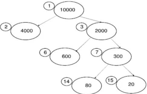
. (3.2)

The tree in Figure 3 will be used to illustrate the difference between d1 and d2. The large ovals in this picture are the deviance at that node, and the small

circles are the leaf number. If observations i and j land in leaves 14 and 15, their d1 distance would be 1.

To calculate the d2 distance, the numerator value isΔDt =10,000−4, 700, which is the root node deviance minus the sum of the leaf nodes. From the group of trees built, assume max

t (ΔDt)=10, 000. This gives a distance of (5,300/10,000)

= 0.53. If we were calculating the distance between two leaves on the best tree, it would be (10,000/10,000) = 1.

Figure 3. Tree with deviance in large circles and leaf numbers in small circles (from Buttrey, 2006)

3. Tree Distance 3, d3

The third distance metric compares the deviance at the parent node of two observations to the deviance at the tree’s root node. The deviance at the parent is denoted Dt(i,j) and the overall deviance of the tree Dt. The distance is calculated by = 0 if L_t(i)=L_t(j) ΔD ⎧ ⎪ ⎫⎪

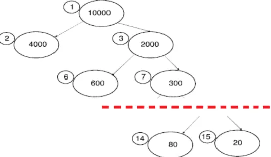
The process to find the d3 distance between leaves 14 and 15 is illustrated in Figure 4. Total change in deviance for the tree is ΔDt= 10,000 − 4,700 =

5,300. After the tree is cropped at the parent node, the change in deviance is

ΔDt(14,15) = 4,900 − 4,700 = 200. The final distance for objects in these leaves

is ΔDt(i,j)

ΔDt

= 200

5300 =0.038. The distance between observations that are close

together on a tree are smaller than those that fall farther apart.

Figure 4. Example tree evaluated using d3 with deviances for leaf 14 and 15 (from Lynch, 2014)

Currently these three distances are computed and stored for all pairs of observations. However, we need only compute distances among all pairs of leaves within each tree, so substantial gains in efficiency will be possible in the future.

C. ALGORITHMS USED

constructs a matrix using Euclidean distance for the numeric datasets and Gower’s dissimilarity for the categorical and mixed datasets. Random forest proximities are used to create the final matrices.

Three clustering algorithms are then used to find a clustering solution, Agnes, PAM and K-means. K-means clustering is only applied to two of the four datasets, which consist of entirely numeric variables. Because its underlying distance is Euclidean. PAM and Agnes are applied to all four datasets using each of the five dissimilarity measures.

Sparse K-means and sparse hierarchical clustering are also used, with sparse K-means applied only to the two numerical datasets.

D. EVALUATION USING CRAMÉR’S V

To compare different clustering approaches, we used four established datasets in which the “correct” classifications are known. The quality of each solution was evaluated using Cramér’s V (Cramér, 1946), which is a scaled version of the χ2 _{measure of association for a two-way table. This produces a}

number between 0 and 1, which will be close to 1 when clusters closely match their class label, and small when they do not.

E. DATASETS

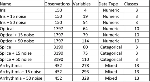
Four datasets from the University of California, Irvine, Machine Learning Repository (Bache & Lichman, 2013) were used in this analysis: Iris, Optical Recognition of Handwritten Digits, Molecular Biology (Splice-junction Gene Sequence), and Cardiac Arrhythmia. The dimensions of each dataset are listed in Table 2. The number of classes k is known and will be used to evaluate how well each algorithm classifies a given set of data. In addition, the algorithms will be run with 2k clusters because the number of clusters might be greater than the number of classes.

Table 2. Dimensions of datasets

Name   Observations   Variables   Data  Type   Classes  

Iris   150   4   Numeric   3  

Iris  +  15  noise   150   19   Numeric   3  

Iris  +  50  noise   150   54   Numeric   3  

Optical   1797   64   Numeric   10  

Optical  +  15  noise   1797   79   Numeric   10  

Optical  +  50  noise   1797   114   Numeric   10  

Splice     3190   60   Categorical   3  

Splice  +  15  noise   3190   75   Categorical   3  

Splice  +  50  noise   3190   110   Categorical   3  

Arrhythmia   452   278   Mixed   13  

Arrhythmia+  15  noise   452   293   Mixed   13  

Arrhythmia  +  50  noise   452   328   Mixed   13  

Noise variables are added to see if the algorithm can discern which variables are most important. Therefore, we will introduce 15 and 50 noise variables into each dataset to see how our algorithms perform.

1. Iris

The Iris flower dataset was made famous by Sir Ronald Fisher (Fisher, 1936) and includes information to quantify the variations of iris flowers of three related species. There are 50 samples from each species (Iris setosa, Iris virginica, and Iris versicolor) collected from the Gaspe Peninsula. Measurements were taken of four features of the flowers, the length and width of their sepals and petals in centimeters. Fisher developed a linear discriminant model to distinguish each species from the other and this dataset has been used as a typical test case for many classification techniques. All variables in this dataset are numeric.

Random noise is introduced into the dataset from a normal distribution with a mean of zero and standard deviation of one.

2. Optical

The Optical Recognition of Handwritten Digits dataset was donated by E. Alpaydin and C. Kaynak (Bache & Lichman, 2013). The data is from 43 people who contributed handwritten digits from zero to nine. These were then converted to bitmaps and a preprocessing program was used to determine what number was displayed. The output is an 8 x 8 matrix of 64 integers taking values zero through 16 to account for small distortions in the way different people write their numbers. There are 5,620 observations total, but only 1,797, the original test set, are used in this analysis. All sixty-four variables are numeric.

Noise variables are introduced by a random sample with replacement, of integers zero through 16.

3. Splice

The Splice-junction data comes from Genbank 64.1 (Bache & Lichman, 2013). It includes 3,190 primate DNA sequences with 60 elements. Each element corresponds to a categorical variable with levels C, A, G and T. The purpose of each is to recognize the boundaries between exons (EI) and introns (IE) to determine if the sequence is from a donor or acceptor, respectively. The third class in this dataset is neither. The sixty variables in this dataset are categorical.

The noise variables for splice are generated by drawing from a random sample with replacement, of the letters C, A, G and T, which correspond to DNA sequence elements.

4. Cardiac Arrhythmia

The final dataset comes from H. Altay Guvenir (Bache & Lichman, 2013) of Bilkent University. The variables in the data comprise the electrocardiograph readings from 452 medical patients. The output of these readings contain 279 variables, of which 206 are numeric and 73 categorical. There are 16 response classes with one being normal cardiac function, one undetermined and the rest

denoting differing degrees of cardiac arrhythmia. Only 13 classes are used in the analysis because three of the classes have no patients associated with them.

Noise variables are introduced from a normal distribution with mean of zero and standard deviation of one.

IV. ANALYSIS

A. INTRODUCTION

This chapter presents the results of our comparative analysis of the different dissimilarity measures and clustering algorithms. Cramér’s V is the metric used for each algorithm and dataset combination, and a higher value indicates a better pairing, with a value of one being a perfect match between clusters and classes.

There are a total of five dissimilarity measuring techniques, three clustering algorithms and two methods that wrap the distance and clustering together. The distance measures are the traditional daisy method, the newer random forest technique and our proposed distances d1, d2, and d3. The three clustering algorithms are Agnes, PAM and K-means. K-means is used only with numeric datasets Iris and optical digits. The two sparse methods, K-means sparse and hierarchical sparse, combine the distance calculation and clustering using techniques previously described.

B. RESULTS

This analysis was done on a MacBook Pro with a 2.6Ghz Intel Core i7 running 16GB of RAM. R Studio with R version 3.1.1 (R Core Team, 2014) was used execute the code. For each dataset, two sets of noise variables are added. Daisy dissimilarity is then computed for all datasets (for the numeric datasets Iris and optical digits, the daisy dissimilarity is Euclidean distance). Random forest proximities and d1 through d3 distances are also computed for all datasets. All were used in Agnes and PAM clustering algorithms. All of the techniques were computationally tractable, and the time to run each one was less than five minutes. Sparse K-means was run only on the two numerical datasets, Iris and optical digits, and took less than 10 minutes on each. Sparse hierarchical clustering was quick, except on optical digits, which took about an hour to run.

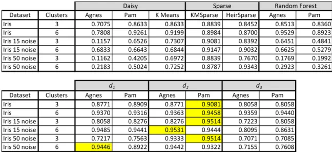
For the Iris dataset shown in Table 3, d2 produces the highest Cramér’s V values (highlighted in yellow) independent of the clustering algorithm. The best clustering results are produced when d2 is paired with PAM (highlighted in yellow). In the dataset with 15 noise variables and run using 2K clusters, Agnes produces a slightly better solution than PAM. Using 50 noise variables and 2K clusters, d1 clustered with Agnes also produces a slightly better solution.

Table 3. Iris Dataset Results

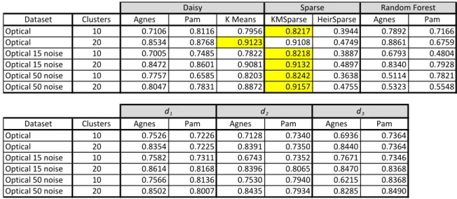
The second numerical dataset in Table 4, optical digits, favors sparse K -means. The new distance metrics perform well, but sparse K-means beats them by a small margin. Even in the presence of noise, the sparse K-means algorithm maintained its advantage because it is able to minimize the contribution of variables that add no value to a dissimilarity calculation.

Dataset Clusters Agnes Pam K0Means KMSparse HeirSparse Agnes Pam Iris 3 0.7075 0.8633 0.8633 0.8839 0.8452 0.8513 0.8360 Iris 6 0.7808 0.9261 0.9199 0.8984 0.8700 0.9529 0.8923 Iris0150noise0variables3 0.1157 0.6526 0.7307 0.9081 0.8392 0.6451 0.4841 Iris0150noise0variables6 0.6833 0.6643 0.6844 0.9147 0.9032 0.6625 0.5279 Iris0500noise0variables3 0.1162 0.4205 0.6972 0.8839 0.7670 0.1769 0.1992 Iris0500noise0variables6 0.2183 0.5024 0.7252 0.8787 0.9343 0.2923 0.3261

Dataset Clusters Agnes Pam Agnes Pam Agnes Pam Iris 3 0.8771 0.8909 0.8771 0.9081 0.8058 0.8058 Iris 6 0.9370 0.9316 0.9363 0.9458 0.9359 0.9440 Iris0150noise0variables3 0.8058 0.8276 0.8276 0.9514 0.7223 0.8058 Iris0150noise0variables6 0.9485 0.9441 0.9531 0.9444 0.8095 0.8631 Iris0500noise0variables3 0.7217 0.7563 0.9333 0.9514 0.7071 0.7085 Iris0500noise0variables6 0.9446 0.8922 0.9442 0.9322 0.7155 0.7608 Random0Forest d1 d2 d3 Daisy Sparse

Table 4. Optical Digits Dataset Results

The Splice dataset in Table 5 is categorical, so the K-means and sparse K-means algorithms are not used. With this dataset, d2 clearly outperformed other techniques. The introduction of noise brought small improvements, due to the automatic variable selection offered by the algorithm.

Table 5. Splice Dataset Results

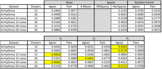
Cardiac arrhythmia was the final dataset shown in Table 6. It contained mixed variable types and performed best with the tree distances. This was the

Dataset Clusters Agnes Pam K0Means KMSparse HeirSparse Agnes Pam Optical 10 0.7106 0.8116 0.7956 0.8217 0.3944 0.7892 0.7166 Optical 20 0.8534 0.8768 0.9123 0.9108 0.4749 0.8861 0.6759 Optical0150noise 10 0.7005 0.7485 0.7822 0.8218 0.3887 0.6793 0.4804 Optical0150noise 20 0.8472 0.8601 0.9081 0.9132 0.4897 0.8340 0.7928 Optical0500noise 10 0.7757 0.6585 0.8203 0.8242 0.3638 0.5114 0.7821 Optical0500noise 20 0.8047 0.7831 0.8872 0.9157 0.4755 0.5323 0.5548

Dataset Clusters Agnes Pam Agnes Pam Agnes Pam Optical 10 0.7526 0.7226 0.7128 0.7340 0.6936 0.7364 Optical 20 0.8354 0.7225 0.8391 0.7350 0.8440 0.7364 Optical0150noise 10 0.7582 0.7311 0.6743 0.7352 0.7671 0.7346 Optical0150noise 20 0.8614 0.8168 0.8396 0.8065 0.8470 0.8368 Optical0500noise 10 0.7566 0.8136 0.7530 0.7940 0.6215 0.8368 Optical0500noise 20 0.8502 0.8007 0.8435 0.7934 0.8285 0.8490 Random0Forest d1 d2 d3 Daisy Sparse

Dataset Clusters Agnes Pam K0Means KMSparse HeirSparse Agnes Pam Splice 3 0.3600 0.1782 0.0617 0.0631 0.0893 Splice 6 0.3603 0.3038 0.0877 0.1206 0.1283 Splice0150noise 3 0.2609 0.1786 0.0617 0.1994 0.1480 Splice0150noise 6 0.2877 0.2638 0.0982 0.2578 0.1358 Splice0500noise 3 0.2329 0.1600 0.0145 0.0668 0.0858 Splice0500noise 6 0.2901 0.2353 0.0398 0.1515 0.1138

Dataset Clusters Agnes Pam Agnes Pam Agnes Pam Splice 3 0.5943 0.5017 0.5977 0.7815 0.0419 0.5647 Splice 6 0.5971 0.6040 0.8249 0.7988 0.0664 0.5952 Splice0150noise 3 0.6104 0.5174 0.6347 0.7677 0.0359 0.6092 Splice0150noise 6 0.6128 0.6130 0.8312 0.7982 0.5738 0.6358 Splice0500noise 3 0.6104 0.5174 0.6347 0.7677 0.0359 0.6092 Splice0500noise 6 0.6128 0.6130 0.8312 0.7982 0.5738 0.6358 Random0Forest d3 d2 d1 Daisy Sparse