Discussion
Papers
In-Sample and Out-of-Sample
Prediction of Stock Market Bubbles
Cross-Sectional Bubbles
Helmut Herwatz and Konstantin A. Kholodilin
1173
Opinions expressed in this paper are those of the author(s) and do not necessarily reflect views of the institute.
IMPRESSUM © DIW Berlin, 2011 DIW Berlin
German Institute for Economic Research Mohrenstr. 58
10117 Berlin
Tel. +49 (30) 897 89-0 Fax +49 (30) 897 89-200
http://www.diw.de
ISSN print edition 1433-0210 ISSN electronic edition 1619-4535
Papers can be downloaded free of charge from the DIW Berlin website:
http://www.diw.de/discussionpapers
Discussion Papers of DIW Berlin are indexed in RePEc and SSRN:
http://ideas.repec.org/s/diw/diwwpp.html
In-sample and out-of-sample prediction of stock market
bubbles: Cross-sectional evidence
¶
Helmut Herwartz
§Konstantin A. Kholodilin
∗November 11, 2011
Abstract
We evaluate the informational content of ex post and ex ante predictors of periods of excess stock (market) valuation. For a cross section comprising 10 OECD economies and a time span of at most 40 years alternative binary chronologies of price bubble periods are determined. Using these chronologies as dependent processes and a set of macroeconomic and financial variables as explanatory variables, logit regressions are carried out. With model estimates at hand, both in-sample and out-of-sample forecasts are made. Overall, the degree of ex ante predictability is limited if an analyst targets the detection of particular turning points of market valuation. The set of 13 potential predictors is classified in measures of macroeconomic or monetary performance, stock market characteristics, and descriptors of capital valuation. The latter turn out to have strongest in-sample and out-of-sample explanatory content for the emergence of price bubbles. In particular, the price to book ratio is fruitful to improve the ex-ante signalling of stock price bubbles.
Keywords: Stock market bubbles; out-of-sample forecasting; financial ratios; OECD
countries.
JEL classification: G01; G17; E27.
¶We thank Christian Dreger and Hans-Eggert Reimers for their helpful suggestions. Moreover, we thank
Martin Everts for the provision of his Matlab code designed to implement the quarterly Bry-Boschan pro-cedure for the identification of stock price bubbles and Matthias Hartmann and Wieland Hoffmann for computational support and data handling.
§Institut f¨ur Statistik und Okonometrie,¨ Christian-Albrechts-Universit¨at zu Kiel, Germany,
[email protected]. This study was conducted while the first author was a guest researcher at the DIW Berlin. The hospitality and productive research environment of this institution are gratefully acknowledged.
Contents
1 Introduction 1
2 Bubble chronology 2
3 Data 5
4 Ex post and ex ante modeling of bubble periods 8
4.1 Logit approach . . . 8 4.2 In-sample analysis. . . 9 4.3 Out-of-sample analysis . . . 10
5 Empirical results 11
5.1 Modeling the benchmark chronology . . . 11 5.2 A summary evaluation measure . . . 13 5.3 Disaggregated forecasting losses . . . 14
6 Conclusions 16
References 16
List of Tables
1 Data description . . . 21 2 Descriptive statistics (means) by variables and countries . . . 22 3 Results of the panel unit-root tests for the regressors . . . 23 4 Descriptive statistics of periods of speculative bubbles by country and for 6
chronologies . . . 24 5 Estimation and diagnostic results for benchmark bubble chronology HPφ= 1
(II) . . . 25 6 Selected diagnostic results for alternative bubble chronologies and summary
measures . . . 29 7 Prediction . . . 32 8 Diagnostic results for unrestricted logit regressions. . . 34
List of Figures
1 Bubble chronologies II (HP, φ = 1) and V (BB, peak) and the deviations of stock prices from trend, 1969:q1-2010:q2 . . . 37 2 In- and out-of-sample accuracy of forecasting the stock price bubbles,
1
Introduction
Beginning in the 1980s, several investigations of stock return predictability have underscored that the pure random walk poorly describes stock price behavior (Shiller (1981),Fama and French (1988)) and have thereby challenged the Efficient Market Hypothesis in its weak form due to Fama (1965). Since the 1990s, the general consensus is that asset pricing models that incorporate time-varying factors can explain return dynamics more accurately (Fama (1991), Campbell (2000)). Variables, such as dividend yields, earning yields, and earnings-to-dividend ratios, have been shown to indicate future market returns especially at longer horizons (Keim and Stambaugh(1986),Campbell and Shiller(1987,1988),Fama and French (1988,1989)). Macroeconomic variables employed in this type of studies include, for instance, interest rates, the term spread, the default spread, the money supply, expected inflation, consumption-to-wealth ratios and aggregate output (Chen et al. (1986),Campbell and Mankiw (1989), Marathe and Shawky (1994), Mills (1996), Hou et al. (2006), Wong-bangpo and Sharma (2002)). The selection of these covariates is typically motivated from noting that they may affect the two major triggers of asset prices, i.e., cash flows and/or discount rates.
Most studies on stock return predictability are exploring the in-sample explanatory con-tent of predetermined factors. Herwartz and Morales-Arias (2009) show for large cross sections of both developed and emerging stock markets thatin-sample return predictability does not necessarily imply out-of-sample return forecastability. Only a few recent papers provide results on out-of-sample performance of dynamic return models. In this line of em-pirical research, variables such as the dividend-to-earnings and book-to-market ratios as well as detrended consumption-to-wealth ratios and term spreads have been shown to contribute positively to one-period-ahead forecasts of excess returns for the case of the US stock market (Lamont (1998), Lettau and Ludvigson (2001), Campbell and Thompson (2007), Harrasty and Roulet (2000), Rapach et al. (2005),Herwartz and Morales-Arias (2009)). As a matter of fact, the ex ante degree of explanation is generally low indicating small signal-to-noise ratios that are characteristic for stock market returns. For a detailed review of the state
of ex post predictability vs. ex ante forecastability of stock market returns the reader may
consult Herwartz and Morales-Arias(2009).
Noting that economic fundamentals appear to carry only weak ex post and ex ante ex-planatory content for equity price dynamics, (aggregate) asset prices eventually drift apart from the underlying fundamental value. While economists have not yet arrived at a consen-sus on neither the definition of (positive or negative) stock price bubbles nor on their causes and triggers (seeKaizoji and Sornette(2008) with references therein) it is apparent that the emergence of boom and bust cycles has dramatic effects on socioeconomic (global) welfare. For instance, relying on IMF forecasts of cumulated gaps of global output over the period 2008 to 2015,Blanchard(2009) estimates the cost of the recent subprime crisis to an amount of 4.7 trillion US dollars, which has been approximately one third of the nominal US GDP in 2008.
In comparison with the literature on stock return predictability the ex ante detection of excessive over- or underpricing on asset markets establishes a more recent line of empirical research in finance. By far and large these contributions are concerned with the conditional analysis of bubbles on stock markets (e.g.,Christiano et al. (2008)), house markets (Agnello
and Schuknecht (2011) and Dreger and Kholodilin (2011), Rousov´a and van den Noord (2011)) or both (e.g., Borio and Lowe (2002), Helbling and Terrones (2003)) or composite assets constructed from these two markets (e.g., Alessi and Detken (2009), Borio et al. (1994),Gerdesmeier et al.(2010)). While these studies parallel to some extent the in-sample return predictability literature, theex ante explanatory content of real economic aggregates, monetary variables and financial ratios has attracted only minor interest in recent studies. Putting particular emphasis on the issue of model uncertainty, Crespo Cuaresma (2010) undertakes a comprehensive analysis of potential determinants of asset price busts by means of Bayesian model averaging for a large cross section of stock and housing markets in the OECD. While most of his study concerns in-sample description of turning points in price trends, it also provides out-of-sample probability scores for the most recent subprime bust period beginning in 2007:Q1.
The aim of this paper is to identify early warning indicators that help to predict the emergence or burst of stock price bubbles. Our data set covers 10 OECD countries (Australia, France, Germany, Italy, Japan, Netherlands, Spain, Switzerland, UK, and the USA) and the time period from 1st quarter 1969 through 2nd quarter 2010. In particular, we distinguish the predictive content of macroeconomic or monetary processes, financial ratios, and stock return characteristics and analyse, which of these (groups of) variables are most relevant for
the ex ante prediction of speculative bubbles and of their bursts.
In Section 2 we describe the extraction of alternative bubble chronologies. Data are introduced in Section 3. Section 4 introduces the methodological approach, which is used for the prediction of the asset price bubbles. Section 5 provides the empirical evidence on predictive accuracy of distinguished predictors with regard to various in-sample and out-of-sample loss functions. Section6concludes. An appendix offers some notes on the treatment of stochastic trends and the role of multicolinearity within the logit regression designs.
2
Bubble chronology
Our objective is to identify variables that allow better forecasts of the stock price bubbles. We assume that market participants are interested in detecting stock price accelerations that are not supported by fundamental macroeconomic dynamics. Stock price increasesper seare a normal phenomenon accompanying any economic expansion. They turn to be dangerous when they decouple from the underlying economic events and follow their own way upwards. When they burst it is often already too late to react. As we know too well from the recent experience, the consequences of price busts can be devastating. Therefore, it is of utmost importance to be able to identify the speculative bubbles when they are still under way and to predict their peaks in advance of their bursting.
Usually, trying to predict bubbles a forecaster can commit two types of errors: i) failing to predict an upcoming bubble or its burst (missing signal) and ii) issuing a false alarm of a bubble that does not emerge at all. Both errors have distinct socioeconomic costs. The costs of a missing signal are immediately obvious when the bubble bursts and eventually triggers a recession with related bankruptcies and increased unemployment. The costs of a false alarm are more difficult to quantify. Firstly, when a false alarm is issued and taken serious, the government may initiate restrictive policies and curb a completely sound expansion.
Thus, its costs are the growth lost due to adoption of untimely measures. Secondly, if the market participants mistake the false alarm as a signal, it may come to a panic ending up in an unintended crisis. This is probably the reason why important stakeholders, like central banks or governments, attach more weight in their loss functions to false alarms than to missing signals. The clearest manifestation of such a behavior was a failure of some political authorities and forecasters in the US to issue a signal of an ongoing recession in 2007 and 2008, despite the clear signals inherent in the leading indicators (Smirnov (2011)). Another example are the overly optimistic forecasts systematically made for the German economy, seeKholodilin and Siliverstovs (2009).
Regardless of the loss function of policy makers, we believe that a timely prediction of stock market bubbles is desirable. For such a prediction we need a bubble chronology allowing to distinguish between i) periods of abnormally rapid growth of stock prices, which typically terminate with a burst followed by drastic downward price corrections, and ii) periods of stock price decline, their eventual recovery, and “normal” increase. The former phase is considered as a bubble, whereas the latter one is treated as a ’no-bubble’ phase.
The determination of a chronology of speculative bubbles is not trivial. Since bubbles are not directly observable, it is difficult to distinguish between the acceleration of stock prices supported by the fundamental factors on the one hand, and excess acceleration spurring price bubbles on the other hand. To extract periods of overvaluation these two components have to be separated in some manner.
Several approaches have been proposed in the literature for the detection of periods of overpricing. As a broad classification one may distinguish approaches that fully rely on univariate filter techniques and detection schemes taking a more structural view on both asset price processes and potential fundamental factors. Regarding the former, filter implied price gaps (see, for instance, Mendoza and Terrones (2008)), cumulated price gaps (e.g., Borio and Lowe (2002), Borio and Lowe (2004)) or forward looking cumulated adjustments (Gerdesmeier et al. (2011)) are used to extract periods of excessive pricing. To account for fundamental factors, for instance, regression models are applied and (cumulated) model residuals are exploited for the detection of bubble periods (e.g.,Terrones and Otrok(2004)). Machado and Sousa (2006) suggest a quantile regression approach. All detection schemes have in common that an analyst must set some threshold parameter that governs the fre-quency of ex post detected periods of excess asset valuation. Providing a further means of cross-checking identified bubble periods, the recent econometric literature addresses the issue of bubble detection by means of testing the random walk hypothesis for log-price series against specifications that allow for explosive stochastic trends (Phillips and Yu (2010) and Homm and Breitung (2009)).
Given the uncertainty about the exact timing of speculative bubbles and the multitude of approaches suggested to generate a bubble chronology, it is sensible to follow distinct approaches or apply alternative threshold parameters. This allows to assess the robustness of conclusions made with regard to potential economic triggers behind the emergence or bust of price bubbles. In this work, we rely on univariate filter techniques, since any regression model linking equity prices and fundamentals may suffer from “spurious causality”. Moreover, when focusing on stock prices it appears overly challenging to determine a set of fundamental
factors that uniformly applies to the entire cross section of considered stock markets.1
Following Mendoza and Terrones(2008) we identify stock price bubbles by means of the Hodrick-Prescott (HP) filter. Formally, a speculative price bubble is determined by means of an indicator function I(•), Rit=I cycit = (Sit−S˜it)> φσci , (1)
where ˜Sit is the HP trend obtained from the actual log stock market indices in time t
and market i, denoted Sit. To estimate the trend component we use λ = 1600 as the
HP smoothing parameter, which is typical for the smoothing of quarterly time series, see Ravn and Uhlig (2002). The unconditional standard deviation of the cyclical component in market i, cycit is denoted σci. Furthermore, in (1) φ is the bubble threshold factor,
determining the degree of overvaluation. If the cyclical component exceeds the predefined threshold, the respective market period is treated as a bubble (Rit = 1). For the purpose
of robustness checking, we choose four alternative threshold values, φ = 0,1,1.5, and 2 to obtain chronologies I to IV. For the most liberal choice, φ = 0, any positive deviation from the trend is regarded as a bubble. While such a classification might be seen as overly liberal it is still of interest if specific economic triggers are behind such market scenarios that might eventually turn into periods of more pronounced asset overevaluation.
As a further robustness check we also determine periods of asset price bubbles by means of a quarterly version of the Bry-Boschan (BB) procedure as implemented inEverts (2006). Originally, this procedure has been suggested to mimic the decision-making process of the National Bureau of Economic Research when determining the turning points of the US busi-ness cycle. In our case, turning points of the stock price cycle are identified analogously. In the first step of the BB algorithm, local minima and maxima are detected. These extreme values are then classified as turning points if they meet several conditions, such as restrictions on the duration of peak-to-trough and peak-to-peak periods, and on the size of the neigh-borhood, over which the local extrema are defined. We use standard settings of the Everts’ code, namely: i) minimum phase duration is 5/3 quarters, ii) minimum cycle duration is 5 quarters, iii) extrema are defined over a neighborhood of 5 quarters, including 2 quarters before and 2 quarters after the local minimum or maximum. Following Crespo Cuaresma (2010), the quarterly BB algorithm is applied to the deviations of the log stock index from the HP trend (cycit), which are smoothed by means of a moving average determined within
a 5-quarter time window. Given the set of turning points resulting from this initial step, we construct two binary chronologies: Firstly, single peak points (Chronology V: BB peak) and, secondly, peaks plus 1 quarter preceding and 1 quarter following each peak (VI: BB peak ±1).
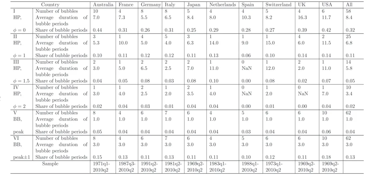
Table 4 reports the total number of speculative bubbles in each country, the average durations of the speculative bubbles, and the frequency of bubble periods by country. For the threshold φ = 1 (Chronology II), the longest speculative price bubbles are observed in the Netherlands (14 quarters) and Switzerland (15 quarters). The bubbles are the shortest in Italy (4 quarters) and Germany (5 quarters). Across chronologies the number of bubbles 1Following a more structural approach with regressing real stock prices on real per-capita GDP and real
interest rates, it turns out that for the stock markets analyzed in this work, regression residuals display similar “trends” in comparison with (univariate) Hodrick-Prescott implied price gaps.
and their durations vary considerably. In fact, the Chronology I is the most liberal one (share of bubbles between 25% and 44%). This chronology generates more signals than the other chronologies. Not surprisingly, the most conservative chronology is that with threshold
φ= 2 (frequencies of bubbles between 0 and 4%). For Bry-Boschan chronologies, where the peaks or the neighborhoods of peaks are examined, the average “peak” duration is artificially set at 1 or 3 quarters.
Figure 1 compares two alternative bubble chronologies with the deviations of the stock prices from their HP trends (thin line). The first chronology (II, HP,φ = 1.0) is represented by the shaded gray area. One can see that it generally reflects periods of substantial stock price increases. Moreover, the ends of bubble periods correspond to peaks of pricing. The second displayed chronology consists of the BB peaks (chronology V, bold lines). They are rather numerous capturing the majority of the local peaks of the stock prices.
3
Data
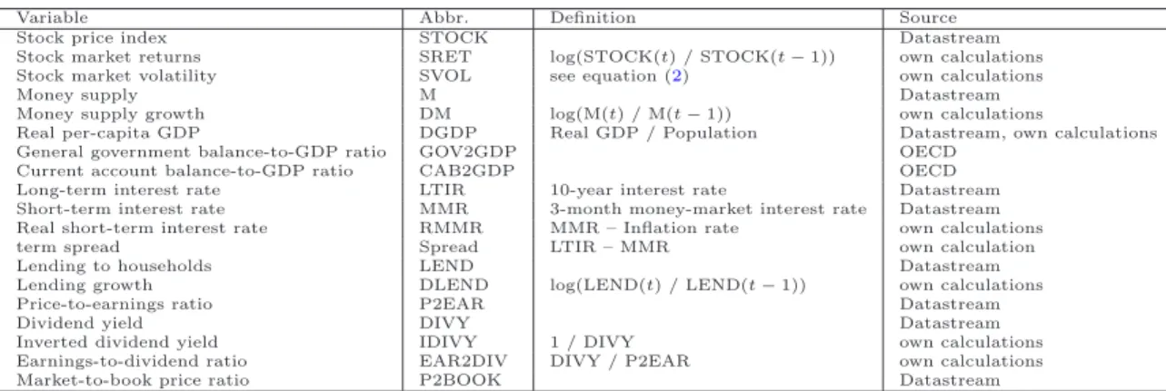
The selection of indicators to explain or predict periods of excess asset valuation, is in-spired by the literature on stock return predictability. Similar to Crespo Cuaresma (2010) we rely on three groups of indicators describing i) the macroeconomic situation (per-capita real GDP growth, government balance-to-GDP ratio, current account balance-to-GDP ra-tio), ii) money or credit market conditions (money supply growth, growth of lending, real money market interest rate, term spread), andiii) capital valuation (price-to-earnings ratio, dividend-to-earning ratios, inverse dividend yield). To the latter group we add the price-to-book ratio. Moreover, following Crespo Cuaresma (2010) we consider stock-market returns as potential triggers of overpricing.
In addition to these first-order processes, we include the realized stock market volatility as a latent second-order characteristic. Formally, the realized stock market volatility prevailing in market i and quarter t is quantified as
RVit = v u u t Mt X m=1 ln Sim Si,m−1 2 , (2)
where m refers to the daily frequency, Mt is the number of trading days in quarter t, and
Sim is the i-th stock market index quoted at day m. The statistic in (2) is a consistent
estimator of the quarterly volatility ifMt → ∞. For practical purposes we regard≈60 daily
price quotes to be sufficient for an accurate quantification of uncertainty prevailing in the stock market (Barndorff-Nielsen and Shephard (2002), Andersen et al. (2003), and Schwert (1989)).2 Apart from consistency, a particular merit of the realized volatility estimator is that
it does not rely on parametric assumptions, which are often used for dynamic formalizations of second-order moment processes as, for example, GARCH (Bollerslev (1986)) or stochastic volatility (Taylor (1986)).
Economic theory and common sense predict the following potential effects of the above variables upon the emergence of stock market overvaluation.
2For Australia, up to the 31st of December 1979, only monthly data on stock indices are available.
Therefore, for the period 1971-1979 the volatility of the Australian stock market is computed based upon monthly stock quotes and beginning with the 1st Quarter 1980 by means of daily quotations.
• Macroeconomic variables. An increase in per-capita income exerts a positive influence on the stock prices reflecting the increased valuation of the enterprises. A growing government balance-to-GDP ratio corresponds to a contractionary fiscal policy, which is typically accompanied by an economic downswing and declining equity prices. In case of the current account balance-to-GDP ratio, it is rather the stock prices that negatively affect the trade balance and not vice versa, as shown in Fratzscher and Straub (2009). However, since we intend to capture longer term price trends, the direction of transitory dependence is of minor importance and we expect a positive impact of the current account balance-to-GDP on the emergence of price booms.
• Monetary variables. Money supply growth is usually assumed to positively contribute
to stock price bubbles, since it is believed to lower interest rates, see Alatiqi and Fazel (2008). Growth of lending may lead to an increase in stock prices, given that loans could be (partly) used to spur equity demand. The real interest rate is typically expected to exert a negative effect upon the stock prices, since it implies an increase of financing costs. Given that increases in the term spread may result from increased long-term or decreased short-term interest rates, its effect upon stock market valuation is indeterminate.
• Financial ratios. Financial ratios are widely used to relate stock valuation with actual
cash flows, profits, or firm values. Since trending fundamental triggers of market performance are likely to impact on both the numerator and the denominator of such ratios, it is likely that the ratio itself is to some degree immunized against trends in fundamentals. From an econometric perspective one might think of such ratios as equilibrium relationships canceling the stochastic trend inherent in stock valuation to obtain a stationary residual. Then, given positive or negative deviations from a steady state, it is of interest which of the variables adjusts more strongly or faster to reestablish the presumed equilibrium. Intuitively, one may expect stock market prices to be more flexible for adjustment in comparison with earnings or dividends. Therefore, financial ratios may carry explanatory or predictive content for periods of excess stock valuation or the burst of bubbles. In this study, financial ratios are determined in a way that stock prices are in the numerator of the ratio. Moreover, we consider the earnings-to-dividend ratio as a potential trigger of price trends.
• Stock market characteristicsA priori one may believe that periods of extreme under- or
overvaluation of assets go along with states of relatively high uncertainty experienced by market participants. Similarly, risk premia are known to establish a positive link between first and second order moments of stock returns. In contrast to expecting a positive relationship between stock market valuation and volatility, one may argue that periods of strong price deterioration go along with markedly increased stock volatility. As a matter of fact, downward price adjustments are known to exert stronger impacts on stock volatility in comparison with positive price changes of comparable size, see Black (1976). Thus, it is an empirical issue to clarify incidence and direction of a potential impact of stock market uncertainty on the upcoming of asset price bubbles. The variables examined in this study, respective data transformations, and data sources are listed in Table 1. Money supply is approximated by means of distinct aggregates, given
that respective quotes are not uniformly documented over distinct countries. The money aggregate M2 is used for Japan and the US. For Australia, France, Germany, Italy, Spain, Switzerland M3 is used, while for the UK we refer to M4. Our study covers 10 OECD countries (Australia, France, Germany, Italy, Japan, Netherlands, Spain, Switzerland, UK, and the USA) and spans the period from the 1st quarter 1969 until the 2nd quarter 2010. Due to the limited data availability the panel is unbalanced. For instance, stock market indices are available over the entire period only for 6 countries out of 10. For the remaining economies the data start much later. In particular, for France stock index data begin as late as the 3rd quarter 1987.
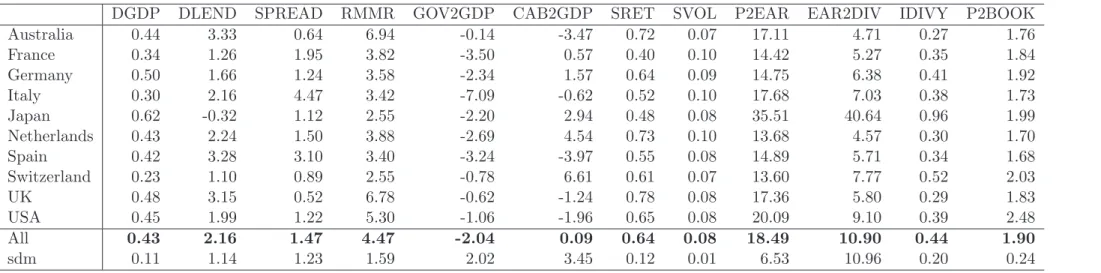
Table 2 reports the country-specific means for all the explanatory variables under in-spection3. In addition, the mean over all the countries and the standard deviation of the
country-specific averages are documented. The real per-capita GDP over all selected coun-tries grew on average at the rate of 0.43% per quarter. It was the highest in Japan (0.62%) and lowest in Italy (0.30%). The lending to households in all countries has been growing by 2.16% per quarter. Interestingly, it was on average negative in Japan, which is possibly a reflection of prolonged deflation. The term spread varied on average between 0.52 percentage points in the UK and 4.47 percentage points in Italy. Overall, in the Anglo-Saxon countries it tends to be lower than the average level of the selected OECD economies. The average real money market interest rate was lowest in Japan and Switzerland (2.55) and highest in Australia (6.94). Again, the Anglo-Saxon economies form a separate group, since their average real money market rates were substantially higher in comparison with the OECD average. The government balance-to-GDP ratio has been mostly negative in all economies under inspection. It is much larger in absolute value than the average in the European con-tinental economies, with the exception of Switzerland. The current account balance-to-GDP variable allows to distinguish two country groupsi) net exporters (France, Germany, Japan, the Netherlands, and Switzerland) and ii) net importers (Australia, Italy, Spain, UK, and the US). The lowest stock market returns have been observed in France (0.40), whereas the highest obtain in the UK (0.78). The stock market volatility has been relatively homoge-nous across markets, varying between 0.07 and 0.10. The price-to-earnings ratio is by far the highest in Japan (35.51), while its lowest values are observed in Switzerland (13.60) and the Netherlands (13.68). The earnings-to-dividend ratios display very high variability: They vary from 4.57 (the Netherlands) to 40.64 (Japan). The inverted dividend-to-yield ratio was the lowest in Australia and the US, while it was by far the highest in Japan. Finally, the average price-to-book ratios are quite similar over distinct markets varying between 1.68 in Spain and 1.99 in Japan.
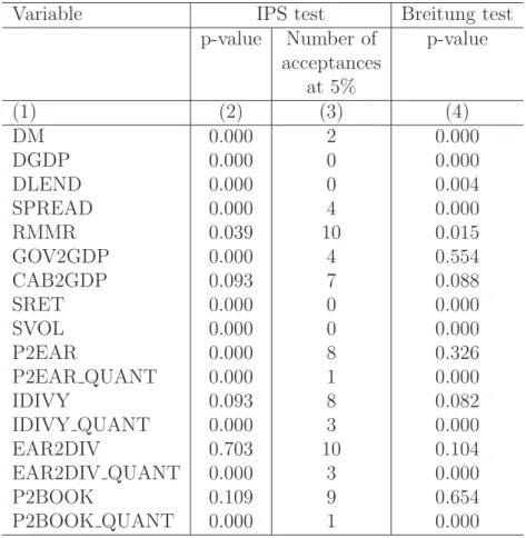
On the one hand, we intend to ensure that the explanatory variables are stationary. Noting that nonstationary processes may divert to any level, reliance on stationary covariates in logit regressions avoids the risk of model implied probability scores that persistently stay close to their bounds of either zero or unity. On the other hand, nonstationary regressors may cointegrate for the generation of ’well behaved’ probability scores (Hu and Phillips (2004),Phillips et al.(2007),Phillips and Yu (2010)). To assess the prevalence of stochastic trends, we conduct panel unit-root tests, namely the Im, Pesaran, and Shin (IPS) (Im et al. 3In fact, these are the variables that turned out to be significant triggers of excess aste valuation in
preliminary analysis. The initial set of variables has been larger. However, descriptive statistics for this enhanced set are not reported here to economize on space.
(2003)) test and the common root test of Breitung (Breitung (2000)). Both tests have the null hypothesis of a unit root prevailing in all panel processes. They differ, however, with regard to the alternative hypothesis. While the alternative of the IPS test allows some fraction of nonstationary panel members under the alternative, the second test is a so-called homogeneous panel unit root test formalizing uniformly stationary panel members under the alternative hypothesis.
The results of panel unit-root tests are reported in Table 3. Columns 2 and 3 document results of the IPS test: the p-value of the test and the number of acceptances of the null hypothesis, that is, the number of economies, for which the ADF p-value exceeds 0.05. One can see that out of 17 variables the null hypothesis of a unit root is accepted only for 4 variables, namely the current account balance-to-GDP ratio, the inverse dividend yield, the earnings-to-dividend ratio, and the price-to-book ratio. At a disaggregate level, for these three variables the unit-root hypothesis is accepted for most markets, with the number of acceptances varying between 7 and 10.
Results for the Breitung test documented in column 4 of Table 3 basically confirm the IPS based diagnosis. The null hypothesis is accepted in 6 cases, 4 of which are the above mentioned stock-market variables plus the price-to-earning ratio in levels, the current account balance-to-GDP ratio, and the government balance-to-GDP ratio.
To summarize, it turns out that financial ratio processes are mostly characterized by high persistence such that common unit root tests underpin the prevalence of stochastic trends for this type of data. Although financial ratios are constructed to represent some equilibrium state, both empirical time series features (persistence and stochastic trends) are well established in the literature (Lewellen (2004), Campbell (1999), and Herwartz and Morales-Arias (2009)).
4
Ex post
and
ex ante
modeling of bubble periods
4.1
Logit approach
As a means to detect and predict periods of excess asset valuation we rely on logit regres-sions.4 Logit regressions allow to determine sign and significance of the influence of each
right hand side variable in predicting periods of speculative bubbles. In general, the logit model is formalized as
P r(Rit= 1|xit) = F(xitβ+εit), i= 1, . . . , N, t= 1, . . . , Ti, (3)
where P r(•) is the conditional probability of a speculative bubble to prevail in market i
and time t, Rit refers to the chronology of the speculative bubbles and xit is the set of
variables considered to have explanatory content for the emergence of price bubbles. The respective parameter vector is β. Moreover, F(•) is the cumulative density function of the logistic distribution and εit is the disturbance term. In order to stress that the sample
information is unbalanced over the cross section dimension we useTito represent the number
of observations available for market i. Throughout, we implement logit models for pooled 4As an alternative, probit regressions turn out to deliver qualitatively identical results throughout.
panel data. Prior to pooling, however, we account for fixed effects by subtracting within-group means from all right hand side variables, except for the constant.
Since the model in equation (3) is specified by means of contemporaneous right-hand-side variables its applicability for ex ante prediction of speculative price bubbles is limited. In fact, such predictions would require corresponding ex ante forecasts of the conditioning variables, which are often subject to (large) prediction errors or difficult to determine at all. Therefore, the following logit regressions with predetermined variables are considered for the purpose of ex ante forecasting:
P r(Rit = 1|xit−p) = F(xit−pβ+εit). (4) In (4), the lag parameter is set top= 1,2 to evaluate theex ante model content at horizons of one and two quarters. As a particular merit of the specification in (4), the collection of conditioning information required for ex ante forecasting is straightforward if the forecast origin dates up to time t.
A particular focus of this study is on the evaluation of model performance with regard to both in-sample (ex post) explanation of periods of excess asset pricing and out-of-sample (ex ante) forecasting thereof. In the following, we briefly describe in-sample and out-of-sample model diagnostics. These are employed to evaluate overall model accuracy and the marginal explanatory content of each right-hand-side variable.
4.2
In-sample analysis
For in-sample diagnosis we consider the following quantities: 1. Pseudo R2
Similar to the degree of explanation in linear models, the goodness of fit for logit models is measured by means of the so-called pseudo R2 suggested in McFadden (1973) and defined as
R2• = 1−L0
L•
1
. (5)
In (5)L0 is the logit likelihood if the right-hand side of the model comprises just a con-stant vector, denotedx(0), andL•1 is the likelihood of some less restricted model specifi-cation indicated by ’•’. We consider three alternative strategies to arrive at alternative model specifications. As the first model to determine L•
1 we use the full set of J = 13 explanatory variables, denoted X = (x(0), x(1), x(2), . . . , x(J)). The second family of models providing L•
1 estimates and indicated with design matrices X(j), j = 1, . . . , J, is obtained from deleting single covariates x(j), from X. The third group of “unre-stricted” models consists of specifications including a constant and single covariates, such that the logit regression design matrix isXj = (x(0), x(j)), j = 1, . . . , J.
2. The quadratic probability score
The accuracy of the alternative conditioning schemes (X, X(j), X
j, j = 1, . . . , J) is
further evaluated by means of the quadratic probability score (QPS), which was sug-gested byBrie(1950) and is widely used in the literature on economic forecasting (e.g.,
Diebold and Rudebusch (1989)). The QPS is defined as QP S• = 1 P iTi N X i=1 T X t=1 (Rit−F(x•i,t−pβˆ • ))2, (6) whereF(x• i,t−pβˆ •
) is the model-derived probability of a speculative bubble to appear in periodt and marketi, ’•’ refers to any specific choice of the right-hand-side regression design (X, X(j), X
j) and the selection ofpcorresponds to the cases of contemporaneous
modeling (p = 0) or the conditioning on lagged information (p = 1,2). QPS varies between 0 and 1. The lower the QPS, the more precise are the predictions of the speculative bubbles. To improve the scale of documented estimation results we report throughout √QP S•.
4.3
Out-of-sample analysis
As a complement to the evaluation of in-sample model accuracy, we conduct an ex ante
evaluation of the logit specifications. For this purpose, particular available observations, comprising the “forecast period” are removed from the sample in a systematic way. Then, estimation ofβis performed by means of sample information, which is presumed to be avail-able to an analyst. Note that the estimator ˆβ• can be seen as a functional of a models’ design matrix (X, X(j), X
j). Then, combining this estimator with the right-hand-side variables
pre-vailing in the “forecast period” yields straightforwardly ex ante probability scores for the event of a price bubble. These scores are translated into binary predictors and then com-pared with actual binary outcomes to assess the predictive accuracy of the model. Similar to in-sample prediction exercises, we determine the overall predictive content of a model using all available covariates (X) and compute the predictive loss that goes along with removing single covariates from this set (X(j)).
Since the data are characterized by a cross sectional and time dimension, we distinguish two directions ofex ante prediction, namely “one-step-ahead” predictions in time and cross-sectional “leave-one-out” forecasts. For the former we use sample information available in some time pointτ to determine probability scores for time periodτ+ 1. For this forecasting exercise right-hand-side variables are subjected to recursive within transformations in order to respect the out-of-sample perspective. For the conditioning in time period τ + 1 we use data observed in time τ+ 1 and centered with the in-sample mean evaluated up to time τ. The first quarter for which predictions are determined is 1993Qu3, thus, 720 out-of-sample forecasts are available for model evaluations. Cross-sectional “leave-one-out” forecasts are computed by means of sample information available for a particular market i coupled with parameter estimates ˆβ• that exploit data collected over the set of 9 remaining markets. Out-of-sample predictions are evaluated in terms of two measures.
1. Henriksson-Merton statistic
The HM-statistic (Henriksson and Merton (1981)) is the sum of two conditional prob-abilities,
HM•
γ = Prob[( ˆR•it> γ)|Rit = 1] + Prob[( ˆR•it < γ)|Rit= 0]. (7)
The conditional probabilities in (7) are determined by means of respective empirical frequencies. HM statistics in excess of unity hint at a positive value of the applied
prediction scheme. For a critical assessment of the informational content of the HM-statistic the reader may consultBlaskowitz and Herwartz (2011). In order to compute the HM-statistic an analyst has to select the probability threshold γ. The higher (smaller) is this threshold, the less (more) bubble periods are identifiedex ante. Thus, the risk of issuing false alarms appears higher for liberal thresholds, while the risk ofex ante missing a bubble period appears more prevalent for conservative, i.e., high levels ofγ. As a consequence, the most suitable selection ofγ depends on the utility function of an analyst. Therefore, the variation of such a threshold should take into account the needs (loss functions) that might characterize heterogeneous market participants. In this work, we select γ in a data-driven way as follows. Suppose an analyst wants to identify “on average” ˜γ×100 percent of “future” observations as bubble periods. To achieve this target approximately we set γ =g1−˜γ, where g1−γ˜ is the (1−γ˜)-quantile of in-sample probability scores. Distinguishing alternative degrees of liberality we set ˜
γ=0.05, 0.10 and ˜γ = 0.20, i.e., an analyst expects price bubbles to occur in one quarter within 5 years, 2.5 years, and 1.25 years, respectively.
2. The ex ante QPS
In full analogy to in-sample diagnosis, the statistic in equation (6) can be determined with reference to predicted rather than estimated probability scores
QP S• = 1 T N X i=1 X τ (Riτ −F(x•i,τ−pβˆ • ))2, (8)
whereT is short for the cardinality of the set of out-of-sample forecasts andF(x•
i,τ−pβˆ •
) is either a one-step-ahead (time) or leave-one-out (market) probability score forecast. A particular advantage of the QPS statistic is that it does not require a probability threshold to translate the metric model predictor into a binaryex ante estimate.
5
Empirical results
In this section, empirical results are discussed firstly with reference to the HP(φ= 1) chronol-ogy (II), which is characterized by an average bubble frequency of ≈14%, and thus, might be seen to compromise between overly liberal and more conservative identification schemes. In-sample estimates and out-of-sample diagnostics are discussed in turn, before correspond-ing results are briefly sketched for the remaincorrespond-ing chronologies (I, III-VI). Mostly, the focus of discussion is on the identification of particularly important (families of) triggers of ex-cess stock market valuation. For the case of most general, unrestricted logit regressions we further take a more detailed view at forecasting losses involved in predicting the alternative chronologies.
5.1
Modeling the benchmark chronology
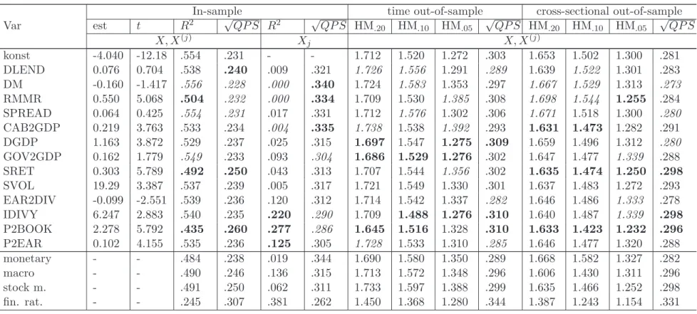
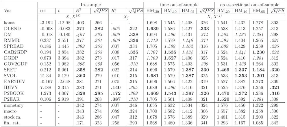
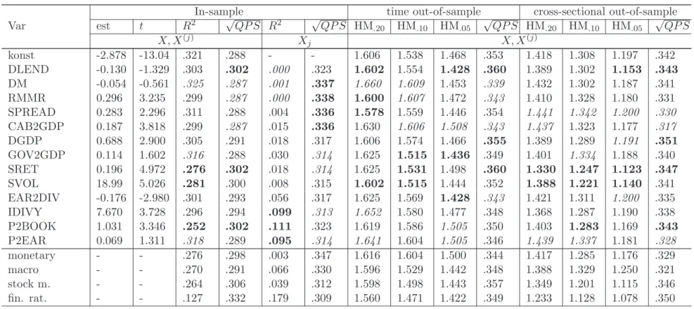
Detailed estimation and prediction results for the third most liberal asset bubble chronology (II, HP,φ = 1) are shown in Table5, where potential explanatory variablesx•
contemporaneously (p= 0, top panel), with a lag of one quarter (p= 1, medium) and a lag of two quarters (p = 2, bottom), respectively. Summary statistics for further chronologies and loss statistics are provided in Tables 4 and 8.
As outlined before, the covariates in the logit design matrix X describe monetary and macroeconomic conditions and further cover financial ratios and stock return characteristics. The RMMR is the only monetary measure that robustly shows explanatory content with 5% significance for bubble determination by means of current or predetermined variables. Simi-larly, DGDP and CAB2GDP turn out to be the most informative macroeconomic measures. In terms of parameter significance, stock return characteristics and financial ratios appear to carry (almost) uniformly informational content for the incidence of stock market overval-uation. The estimated marginal impact of stock market uncertainty on the probability of a price bubble is positive, indicating that excess volatility may hide the emergence of price bubbles.
Coupling a constant with single covariates (Xj) obtains that the informational content of
monetary variables is less than that of macroeconomic measures. “Partial” degrees of expla-nation extracted from such models reveal that financial ratios have, in general, the highest informational content. As documented in Table 5, the degrees of explanation achieved by fully specified logit regressions is 55.4%, 40.3% and 32.1% if right-hand-side variables are measured contemporaneously, with one lag and with two lags, respectively. In comparison with other covariates, removing the price-to-market ratio (P2BOOK) from the set of re-gressors involves the largest deterioration of the pseudo R2 shrinking to 43.5%, 32.9% and 25.2%, respectively. As a confirmation of this result, moreover, the in-sample √QP S mea-sures show the highest upward shift for model specifications leaving out P2BOOK. In this sense, P2BOOK can be seen as the most important measure in explaining the occurrence of price bubbles as classified by the benchmark chronology.
Given the large number of ex ante observations HM-statistics based on unrestricted logit regressions exceed unity with common levels of significance. As one might expect, theex ante
content of the logit regressions is highest (smallest) for specifications with right-hand-side variables measured contemporaneously (with lag of 2 quarters).
To complement the performance measures attached to single covariates, we assess the performance of logit regressions where a constant is coupled with, respectively, 4 monetary aggregates, 3 macroeconomic processes, 2 stock return characteristics, and 4 financial ratios. Moreover, we remove these measures jointly from the full set of covariates to obtain logit designs. Following such lines is thought to uncover the informational content of particular segments of the economy. Regarding the informational content of grouped covariates it becomes evident that the financial ratios are uniformly most relevant for modeling and prediction of periods of excess stock market valuation. Removing these ratios jointly from the set of covariates involves uniformly highest losses in terms of a reduced in-sample R2 and out-of-sample predictive accuracy. For instance, in models with contemporaneous right-hand-side variables, the pseudoR2of 55.4% observed for the fully unrestricted model drops to 24.5% after joint removal of the financial ratios. In relative terms, similar losses are obtained for models with lagged right-hand-side covariates. In relation to the impact of omitting financial ratios the omission of monetary aggregates, macroeconomic processes, and stock market return characteristics is less relevant. In some cases HM-statistics even improve after the joint removal of respective variables. Thus, it appears that the informational
content of such aggregates is less specific and could also be reflected within other economic processes. Ranking the considered segments in terms of their “partial” R2 supports the view that macroeconomic variables are more informative than monetary aggregates or stock return characteristics. However, this ordering is not robust when it comes to a comparative evaluation of ex-ante performance measures.
Figure 2 compares the in-sample (solid line) and out-of-sample (dashed) model-derived probabilities of speculative bubbles based on logit models for the reference chronology (II, HP,φ = 1.0, shaded areas). Due to the limited availability of data on explanatory variables the estimation and forecasting period is generally shorter than the sample period. In-sample probability scores are determined by means of full sample (10 cross-section members) logit modeling with covariates being lagged by one quarter (xi,t−p, p= 1). Out-of-sample scores are obtained after removing single markets from the sample and logit estimation of model parameters by means of sample information from the remaining 9 markets.
In general, logit models accurately predict the stock price bubbles within and out of sample. In fact, the differences between the in- and out-of-sample forecasts are rather minor. It is worth noticing, however, a large discrepancy between the in- and out-of-sample forecast of the US market bubble at the very end of the sample. It can be explained by a rapid acceleration of the price-to-earnings ratio, P2EAR, in 2009. P2EAR jumped from 18.1 in the 2009Qu1 to 61.8 in the 2009Qu2 and then even to 146.2 in the 2009Qu3 and 2009Qu4.
Table 6 sheds light on the robustness of estimation results over the set of alternative bubble chronologies for the unrestricted logit designs. Noting that single parameters in ˆβ are mainly informative with regard to their sign and significance, Table 6 only documents thet-ratios of single parameter estimates. It turns out that over the set of 6 bubble chronolo-gies no single covariate (measured contemporaneously or with lags of one or two quarters) has a uniform and significant impact on the probability of a stock price bubble. Distin-guishing logit specifications with alternative time lags of explanatory variables (one quarter, two quarters, one year), similar results are reported by Crespo Cuaresma (2010). However, for a couple of covariates relatively robust inferential results are available. Conditioning on contemporaneous variables, RMMR, SPREAD, DGDP, GOV2GDP and P2BOOK obtain uniformly positive marginal impacts, that are, except for the impact of RMMR in line with economic expectation. Among predetermined explanatory variables stock returns (SRET) and CA2GDP are characterized by uniformly positive marginal impacts on the logit proba-bility scores.
5.2
A summary evaluation measure
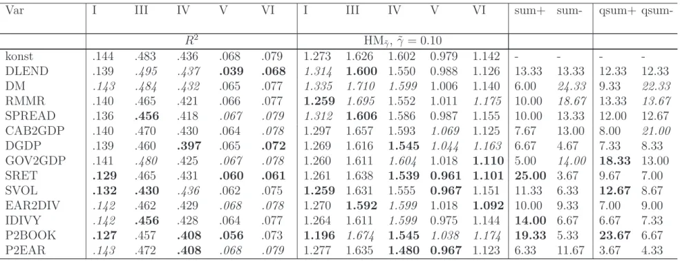
To sketch diagnostic model results for the remaining 5 bubble chronologies Table5documents in-sample pseudoR2 statistics and out-of-sample HM-statistics (γ = 0.1) and their variation when switching from unrestricted model specifications (X) to regressions where single co-variates are removed (X(j)). HM-statistics are determined for the time series out-of-sample analysis since this ex ante dimension might be of more practical interest in comparison with cross-sectional leave-one-out modeling. While the in-sample R2 generally diminishes with the removal of single covariates, its effect on the out-of-sample performance is not uni-form. Depending on the particular bubble chronology the removal of single covariates may eventually foster the predictive strength. When examining the marginal content of single
variables across alternative bubble chronologies it becomes apparent that overall conclusions are hardly available. Therefore, we turn to an aggregate performance assessment.
In total, 12 statistics are used to evaluate the marginal effects of including/excluding (Xj/X(j)) particular covariates in/from the logit design. With regard to in-sample and
out-of-sample diagnostics 4 and 8 statistics are determined, respectively. Among the latter we have 6 HM-statistics (three threshold levels ˜γ and two directions of ex-ante modeling) and 2 QPS measures. Leaving out the constant, the column dimension of the unrestricted logit designs is 13. For an overall assessment of the marginal importance of single co-variates we count how often over all alternative bubble chronologies and model diagnos-tics the inclusion/exclusion (Xj/X(j)) of a particular covariate is among the three most
helpful/detrimental model variations. As a complementary summary measure we further count how often the inclusion/exclusion of a particular variable belongs to the 3 least help-ful/detrimental in comparison over all covariates. While for the former statistic the informa-tional content of a particular variable increases with counts, for the latter it decreases with counts. HM-statistics determined with respect to distinct threshold levels ˜γ are most likely to be highly correlated. To account for this fact, we downweigh the counts for HM-statistics by a factor of 1/3. Thus, the maximum count, obtained if a particular variable belongs throughout to the 3 most helpful/detrimental covariates, is 48 (6 chronologies times 6 statis-tics with full weight and 6 HM-statisstatis-tics with weight 1/3). Conceptually, such success counts are similar to Bayesian assessments of a variable’s informational content. Systematically ag-gregating over posterior distributions, however, Bayesian model inclusion probabilities as documented in Crespo Cuaresma(2010) allow a statistically sound interpretation. Lacking such a methodological underpinning, a particular merit of the less formal count statistics considered here is that they summarize information inherent in a multitude of model diag-nostics that might mimic an analyst’s multidimensional utility function. Overall summary statistics obtained along these lines are shown in the rightmost columns of Table 5.
Although it is not possible to attach any significance levels to the overall evaluation, two observations can be made. First, single covariates do not contribute uniformly to model success. Second, the marginal content of particular covariates differs for models with ex-planatory variables measured simultaneously or with time lags of one or two quarters. In case of contemporaneous conditioning (p= 0), P2BOOK achieves the highest count statistic (22), which exceeds the marginal content signified for other financial ratios (7 to 17). In comparison, the inclusion/exclusion of DM, SPREAD, CAB2GDP, GOV2GDP or SVOL (all with counts below 10) is rarely crucial for model success. Regarding the most help-ful/detrimental predetermined indicators of bubble periods (p = 1,2) confirms the partial content of the P2BOOK and, moreover, hints at SRET and DLEND as further potentially useful predictors. Apparently, the share of instances where these variables are least crucial confirms the outcomes discussed so far, since all respective count statistics are among the smallest and are almost uniformly below 10.
5.3
Disaggregated forecasting losses
Aggregating conditional probabilities the HM-statistic in (7) may hide forecast characteristics that are important with regard to loss functions of particular market participants or other stakeholders. Therefore, Table 6 provides for fully unrestricted logit regressions (design
matrices X) more disaggregated forecast qualifications. The losses are measured in terms of three empirical frequencies, i) the number of correctly predicted bubble periods divided by total bubbles (G1), ii) the number of correctly predicted no-bubble periods divided by total no-bubble periods (G2), and iii) the number of falsely predicted bubbles over all forecasted bubbles (G3). All measures depend on the probability threshold γ =γ(˜γ). While the sum over G1 and G2 is equal to HM, the measure G3 describes the risk of issuing a false alarm. By construction, the frequencies G1 and G2 are positively related to an analyst’s utility and could be better seen as gain functions. The table documents detailed losses for both directions of out-of-sample forecasting, contemporaneous and lagged explanatory variables, 6 bubble chronologies, and three alternative thresholds for translating continuous probability scores into binary estimates.
The following observations can be made: Firstly, the loss diagnostics generally differ to some extent for both directions of out-of-sample modeling. This result hints at the potential of structural model variation over time or at market heterogeneity. Arguably, we cannot attach an explicit significance level to this diagnosis. Respective frequency estimates from time vs. cross-sectional forecasting, however, are hardly in line with a homogeneity assump-tion, since the number of out-of-sample observations is rather large and, thus, the standard errors of frequency estimates are likely small. Secondly, while the prediction schemes per-form rather accurately in correctly signaling no-bubble periods, the modeling perper-formance is more heterogeneous in terms of the successful prediction of bubble periods. Throughout,G2 statistics are close to or in excess of 0.8, and thus, reflect that the threshold parameter ˜γ is set to obtain relatively rarely out-of-sample indications of price bubbles. Thirdly, targeting at the time precise ex-ante identification of turning points (Chronology V) is hardly suc-cessful. For this chronology we obtain relatively small success frequencies of issuing correct bubble signals (7% to 30%, G1), and relatively large frequencies of false signals (88% to 94%, G3). For the more liberal BB based chronology (VI) both disaggregated loss functions improve to some extent (7% to 39% for G1, and 62% to 86% for G3). Fourthly, taking a particular view at loss measures G1 andG3, one may argue that prediction schemes should accord with the requirement G1 > G3. It turns out that this condition does not apply generally for the more conservative chronologies (IV to VI). For the more liberal schemes of bubble periods (I to III) and when setting liberal probability thresholds (˜γ = 0.1, 0.2) al-most all frequencies of false alarms are less than those of correctly predicted bubble periods. Finally, it is intuitive to observe that contemporaneous modeling (p = 0) achieves overall highest degrees of “out-of-sample” utility. It is worth noticing, however, that additional losses that can be attributed to the modeling with predetermined variables (p = 1,2) are moderate throughout. As a possible explanation of this result one could imagine that with distinct time horizons differentiated impacts of the considered monetary, macroeconomic, and financial factors come into effect. Arguably, such an explanation is also supported by the hetergeneous patterns of success counts documented in the right hand side columns of Table 6.
6
Conclusions
In this paper, we constructed country-specific chronologies of price bubbles for 10 OECD economies (Australia, France, Germany, Italy, Japan, Netherlands, Spain, Switzerland, UK, and the USA) over the period 1969:Q1-2010:Q2. These chronologies are obtained by means of alternative filter approaches.
While logit regression models show statistically significant nontrivial predictive content, their economic significance is limited in particular for the most conservative bubble chronolo-gies. For the establishment of an early warning system the translation of out-of-sample prob-ability scores into binary forecasts (bubble or no bubble) is likely to suffer from the issuance of false alarms. Over distinct bubble chronologies and conditioning on contemporaneous vs predetermined explanatory variables we do not obtain any covariate that shows a uniform relation to model implied probability scores. The same applies for the contribution of single covariates to a plentitude of considered loss functions. Comparing the informational content of distinct (groups of) predictors we find that financial ratios are more informative in com-parison with monetary aggregates, macroeconomic processes or stock return characteristics. From the set of alternative financial ratios the price-to-book ratio appears to carry strongest content for the identification of periods of excess stock market valuation with regard to both in-sample and out-of-sample modeling. Among the set of macroeconomic indicators we find evidence for a particular strength of per capita growth of GDP in contemporaneous mod-elling. In addition, Stock market returns lagged by one or two quarters carry specific ex ante content.
Comparing the results of time series and cross-sectional out-of-sample exercises, it ap-pears that the emergence of price bubbles may display market-specific characteristics. We consider the detection and exploitation of such heterogeneities as an issue of future research. Moreover, apart from market specific conditional characteristics of stock overvaluation, our evidence suggests that instances or periods of excess asset pricing, might be the result of some heterogenous coincidence of monetary or macroeconomic states, stock market or capi-tal valuation characteristics. Thus, it appears sensible to take real time perspectives on the procession of news entering the financial markets in order to improve early warning schemes. In this venue of future research higher frequency or mixed frequency approaches might be of particular interest.
References
Agnello, L. and L. Schuknecht (2011). Booms and busts in housing markets: Determinants and implications. Journal of Housing Economics 20(3), 171–190.
Alatiqi, S. and S. Fazel (2008). Can money supply predict stock prices? Journal for
Economic Educators 8(2), 54–59.
Alessi, L. and C. Detken (2009). Real time’s early warning indicators for costly asset price boom/bust cycles — a role for global liquidity. Working Paper Series 1039, European Central Bank.
Andersen, T. G., T. Bollerslev, F. X. Diebold, and P. Labys (2003). Modeling and forecasting realized volatility. Econometrica 71(2), 579–625.
Barndorff-Nielsen, O. E. and Shephard (2002). Econometric analysis of realized volatility and its use in estimating stochastic volatility models. Journal of The Royal Statistical
Society Series B 64(2), 253–280.
Black, F. (1976). Studies in stock price volatility changes. InProceedings of the 1976
Meet-ing of the Business and Economics Statistics Section, pp. 177–181. American Statistical
Association.
Blanchard, O. (2009). The crisis: Basic mechanisms and appropriate policies. CESifo
Forum 10(1), 3–14.
Blaskowitz, O. and H. Herwartz (2011). On economic evaluation of directional forecasts.
International Journal of Forecasting 27(4), 1058–1065.
Bollerslev, T. (1986). Generalized autoregressive conditional heteroskedasticity. Journal of
Econometrics 31, 307–327.
Borio, C., N. Kennedy, and S. D. Prowse (1994). Exploring aggregate asset price fluctua-tions across counties, measurement, determinants, and monetary policy implicafluctua-tions. BIS Economic Papers.
Borio, C. and P. Lowe (2002). Asset prices, financial and monetary stability: exploring the nexus. BIS Working Papers N 114.
Borio, C. and P. Lowe (2004). Securing sustainable price stability: should credit come back from the wilderness? Bank for International Settlements Working Papers No 157.
Breitung, J. (2000). The local power of some unit root tests for panel data. In B. Balt-agi (Ed.), Nonstationary Panels, Panel Cointegration, and Dynamic Panels. Advances in
econometrics, pp. 161–178. Elsevier Science.
Brie, G. W. (1950). Verification of forecasts expressed in terms of probability. Monthly
Weather Review 78(1), 1–3.
Campbell, J. (2000). Asset pricing at the millennium.The Journal of Finance 55, 1515–1567. Campbell, J. and N. Mankiw (1989). Consumption, income and interest rates: Reinterpreting
the time series evidence. NBER macroeconomics annual, 185–216.
Campbell, J. and R. Shiller (1987). Cointegration and tests of present value models. Journal
of Political Economy 5, 1062–1088.
Campbell, J. and R. Shiller (1988). The dividend-price ratio and expectations of future dividends and discount factors. Review of Financial Studies 1, 195–228.
Campbell, J. and S. Thompson (2007). Predicting excess returns out-of-sample: Can any-thing beat the historical average? Review of Financial Studies 41, 27–60.
Campbell, J. Y. (1999). Handbook of Macroeconomics, Volume 1, Chapter 19 Asset prices, consumption, and the business cycle, pp. 1231–1303. Elsevier.
Chen, N., R. Roll, and S. Ross (1986). Economic forces and the stock market. The Journal
of Business 59, 383–403.
Christiano, L., C. Ilut, R. Motto, and M. Rostagno (2008). Monetary policy and stock market boom-bust cycles. Working Paper Series 955, European Central Bank.
Crespo Cuaresma, J. (2010). Can emerging asset price bubbles be detected? OECD Eco-nomics Department Working Papers 772, OECD Publishing.
Diebold, F. X. and G. D. Rudebusch (1989). Scoring the leading indicators. Journal of
Business 62, 369–402.
Dreger, C. and K. Kholodilin (2011). An early warning system to predict the house price bubbles. DIW Berlin Discussion Paper 1142.
Everts, M. (2006). Duration of business cycles. MPRA Paper 1219, University Library of Munich, Germany.
Fama, E. (1965). The behaviour of stock-market prices. The Journal of Business 38, 34–105. Fama, E. (1991). Efficient capital markets II. The Journal of Finance 46, 1575–1617. Fama, E. and K. French (1988). Dividend yields and expected returns. Journal of Financial
Economics 2, 3–25.
Fama, E. and K. French (1989). Business conditions and expected returns on stocks and bonds. Journal of Financial Economics 25, 23–49.
Fratzscher, M. and R. Straub (2009). Asset prices and current account fluctuations in g7 economies. Working Paper Series 1014, European Central Bank.
Gerdesmeier, D., H.-E. Reimers, and B. Roffia (2010). Asset price misalignments and the role of money and credit. International Finance 13(3), 377–407.
Gerdesmeier, D., H.-E. Reimers, and B. Roffia (2011). Early warning indicators for asset price booms. Review of Economics and Finance 3, 1–19.
Harrasty, R. and J. Roulet (2000). Modeling stock market returns. Journal of Portfolio
Management 26, 33–46.
Helbling, T. and M. E. Terrones (2003). Real and financial effects of bursting asset price bubbles. IMF World Economic Outlook.
Henriksson, R. D. and R. C. Merton (1981). On market timing and investment performance. ii. statistical procedures for evaluating forecasting skills. Journal of Business 54(4), 513– 33.
Herwartz, H. and L. Morales-Arias (2009). In-sample and out-of-sample properties of in-ternational stock return dynamics conditional on equilibrium pricing factors. European
Journal of Finance 15(1), 1–28.
Homm, U. and J. Breitung (2009). Testing for speculative bubbles in stock markets. a comparison of alternative methods. mimeo.
Hou, K., G. Karolyi, and B. Kho (2006). What fundamental factors drive global stock returns?
Hu, L. and P. C. B. Phillips (2004). Nonstationary discrete choice. Journal of
Economet-rics 120(1), 103–138.
Im, K. S., M. H. Pesaran, and Y. Shin (2003). Testing for unit roots in heterogeneous panels.
Journal of Econometrics 115(1), 53–74.
Kaizoji, T. and D. Sornette (2008). Market bubbles and crashes. Quantitative Finance Papers 0812.2449, arXiv.org.
Keim, D. and R. Stambaugh (1986). Predicting returns in the stock and bond markets.
Journal of Financial Economics 17, 357–390.
Kholodilin, K. A. and B. Siliverstovs (2009). Do forecasters inform or reassure? evaluation of the german real-time data. Applied Economics Quarterly (formerly:
Konjunkturpoli-tik) 55(4), 269–294.
Lamont, O. (1998). Earnings and expected returns. Journal of Finance 53, 1563–1587. Lettau, M. and S. Ludvigson (2001). Consumption, aggregate wealth and expected returns.
Journal of Finance 56, 815–849.
Lewellen, J. (2004). Predicting returns with financial ratios. Journal of Financial
Eco-nomics 74(2), 209–235.
Machado, J. F. and J. Sousa (2006). Identifying asset price booms and busts with quan-tile regressions. Working Papers w200608, Banco de Portugal, Economics and Research Department.
Marathe, A. and H. Shawky (1994). Predictability of stock returns and output. Quarterly
Review of Economics and Finance 34, 317–331.
McFadden, D. (1973). Conditional logit analysis of qualitative choice behavior. In P. Zarem-bka (Ed.),Frontiers in Econometrics, Volume 1, pp. 105–142. Academic Press.
Mendoza, E. G. and M. E. Terrones (2008). An anatomy of credit booms: Evidence from macro aggregates and micro data. NBER Working Papers 14049.
Mills, T. (1996). The econometrics of the ’market model’: Cointegration, error correction and exogeneity. International Journal of Finance and Economics 1, 275–286.
Phillips, P. and J. Yu (2010). Dating the timeline of financial bubbles during the subprime crisis. Cowles Foundation Discussion Papers 1770, Cowles Foundation for Research in Economics, Yale University.
Phillips, P. C., S. Jin, and L. Hu (2007). Nonstationary discrete choice: A corrigendum and addendum. Journal of Econometrics 141(2), 1115–1130.
Rapach, D., M. Wohar, and J. Rangvid (2005). Macro variables and international return predictability. International Journal of Forecasting 21, 137–166.
Ravn, M. O. and H. Uhlig (2002). On adjusting the Hodrick-Prescott filter for the frequency of observations. The Review of Economics and Statistics 84(2), 371–375.
Rousov´a, L. and P. van den Noord (2011). Predicting peaks and troughs in real house prices. OECD Economics department working paper no. 882.
Schwert, G. W. (1989). Why does stock market volatility change over time? Journal of
Finance 44(5), 1115–53.
Shiller, R. (1981). Do stock prices move too much to be justified by subsequent changes in dividends? American Economic Review 71, 421–436.
Smirnov, S. V. (2011). Discerning “turning points” with cyclical indicators: A few lessons from “real time” monitoring the 2008-2009 recession. Higher School of Economics Working Paper WP2/2011/03.
Taylor, S. (1986). Modeling financial time series. John Wiley, Chichester.
Terrones, M. and C. Otrok (2004). The global house price boom. IMF World Economic
Outlook, 71–136.
Wongbangpo, P. and S. Sharma (2002). Stock market and macroeconomic fundamentals dynamic interactions: ASEAN-5 countries. Journal of Asian Economics 13, 27–51.
Appendix
Table 1: Data description
Variable Abbr. Definition Source Stock price index STOCK Datastream Stock market returns SRET log(STOCK(t) / STOCK(t−1)) own calculations Stock market volatility SVOL see equation (2) own calculations Money supply M Datastream Money supply growth DM log(M(t) / M(t−1)) own calculations
Real per-capita GDP DGDP Real GDP / Population Datastream, own calculations General government balance-to-GDP ratio GOV2GDP OECD
Current account balance-to-GDP ratio CAB2GDP OECD Long-term interest rate LTIR 10-year interest rate Datastream Short-term interest rate MMR 3-month money-market interest rate Datastream Real short-term interest rate RMMR MMR – Inflation rate own calculations term spread Spread LTIR – MMR own calculation Lending to households LEND Datastream Lending growth DLEND log(LEND(t) / LEND(t−1)) own calculations Price-to-earnings ratio P2EAR Datastream Dividend yield DIVY Datastream Inverted dividend yield IDIVY 1 / DIVY own calculations Earnings-to-dividend ratio EAR2DIV DIVY / P2EAR own calculations Market-to-book price ratio P2BOOK Datastream
Table 2: Descriptive statistics (means) by variables and countries
DGDP DLEND SPREAD RMMR GOV2GDP CAB2GDP SRET SVOL P2EAR EAR2DIV IDIVY P2BOOK
Australia 0.44 3.33 0.64 6.94 -0.14 -3.47 0.72 0.07 17.11 4.71 0.27 1.76 France 0.34 1.26 1.95 3.82 -3.50 0.57 0.40 0.10 14.42 5.27 0.35 1.84 Germany 0.50 1.66 1.24 3.58 -2.34 1.57 0.64 0.09 14.75 6.38 0.41 1.92 Italy 0.30 2.16 4.47 3.42 -7.09 -0.62 0.52 0.10 17.68 7.03 0.38 1.73 Japan 0.62 -0.32 1.12 2.55 -2.20 2.94 0.48 0.08 35.51 40.64 0.96 1.99 Netherlands 0.43 2.24 1.50 3.88 -2.69 4.54 0.73 0.10 13.68 4.57 0.30 1.70 Spain 0.42 3.28 3.10 3.40 -3.24 -3.97 0.55 0.08 14.89 5.71 0.34 1.68 Switzerland 0.23 1.10 0.89 2.55 -0.78 6.61 0.61 0.07 13.60 7.77 0.52 2.03 UK 0.48 3.15 0.52 6.78 -0.62 -1.24 0.78 0.08 17.36 5.80 0.29 1.83 USA 0.45 1.99 1.22 5.30 -1.06 -1.96 0.65 0.08 20.09 9.10 0.39 2.48 All 0.43 2.16 1.47 4.47 -2.04 0.09 0.64 0.08 18.49 10.90 0.44 1.90 sdm 0.11 1.14 1.23 1.59 2.02 3.45 0.12 0.01 6.53 10.96 0.20 0.24
Note: sdm stands for standard deviation of country-specific means. For a listing of variables see Table 1.
Table 3: Results of the panel unit-root tests for the regressors
Variable IPS test Breitung test
p-value Number of p-value acceptances at 5% (1) (2) (3) (4) DM 0.000 2 0.000 DGDP 0.000 0 0.000 DLEND 0.000 0 0.004 SPREAD 0.000 4 0.000 RMMR 0.039 10 0.015 GOV2GDP 0.000 4 0.554 CAB2GDP 0.093 7 0.088 SRET 0.000 0 0.000 SVOL 0.000 0 0.000 P2EAR 0.000 8 0.326 P2EAR QUANT 0.000 1 0.000 IDIVY 0.093 8 0.082 IDIVY QUANT 0.000 3 0.000 EAR2DIV 0.703 10 0.104 EAR2DIV QUANT 0.000 3 0.000 P2BOOK 0.109 9 0.654 P2BOOK QUANT 0.000 1 0.000
Table 4: Descriptive statistics of periods of speculative bubbles by country and for 6 chronologies
Country Australia France Germany Italy Japan Netherlands Spain Switzerland UK USA All
I Number of bubbles 10 4 8 8 5 4 4 5 4 6 58
HP, Average duration of bubble periods
7.0 7.3 5.5 6.5 8.4 8.0 10.3 8.2 16.3 11.7 8.4
φ= 0 Share of bubble periods 0.44 0.31 0.26 0.31 0.25 0.29 0.28 0.27 0.39 0.42 0.32
II Number of bubbles 3 1 4 5 3 1 1 1 4 2 25
HP, Average duration of bubble periods
5.3 10.0 5.0 4.0 6.3 14.0 9.0 15.0 6.0 11.5 6.8
φ= 1 Share of bubble periods 0.10 0.11 0.12 0.12 0.11 0.13 0.06 0.10 0.14 0.14 0.11
III Number of bubbles 2 1 2 2 2 1 0 1 2 1 14
HP, Average duration of bubble periods
3.0 5.0 6.5 2.5 7.0 11.0 NaN 12.0 2.0 11.0 5.8
φ= 1.5 Share of bubble periods 0.04 0.05 0.08 0.03 0.08 0.10 0.00 0.08 0.02 0.07 0.05
IV Number of bubbles 1 1 2 1 2 1 0 1 0 1 10
HP, Average duration of bubble periods
3.0 4.0 2.5 2.0 3.5 4.0 NaN 2.0 NaN 7.0 3.4
φ= 2 Share of bubble periods 0.02 0.04 0.03 0.01 0.04 0.04 0.00 0.01 0.00 0.04 0.02
V Number of bubbles 8 4 6 7 6 4 5 6 6 10 62
BB, Average duration of bubble periods
1.0 1.0 1.0 1.0 1.0 1.0 1.0 1.0 1.0 1.0 1.0
peak Share of bubble periods 0.05 0.04 0.04 0.04 0.04 0.04 0.03 0.04 0.04 0.06 0.04
VI Number of bubbles 8 4 6 7 6 4 5 6 6 10 62
BB, Average duration of bubble periods
3.0 3.0 3.0 3.0 3.0 3.0 3.0 3.0 3.0 3.0 3.0
peak±1 Share of bubble periods 0.15 0.13 0.11 0.13 0.11 0.11 0.10 0.12 0.11 0.18 0.13
Sample 1971q1-2010q2 1987q3-2010q2 1991q2-2010q2 1981q2-2010q2 1969q2-2010q2 1983q1-2010q2 1988q1-2010q2 1973q1-2010q2 1969q2-2010q2 1969q2-2010q2 24