Visual Odometry using Convolutional Neural Networks

(1)

The Kennesaw Journal of Undergraduate Research

Volume 5 Issue 3

Article 5

December 2017

Visual Odometry using Convolutional Neural Networks

Alec Graves

Kennesaw State University, [email protected]

Steffen Lim

Thomas Fagan

Kevin McFall PhD.

Follow this and additional works at: https://digitalcommons.kennesaw.edu/kjur

Part of the Artificial Intelligence and Robotics Commons

Recommended Citation

Graves, Alec; Lim, Steffen; Fagan, Thomas; and McFall, Kevin PhD. (2017) "Visual Odometry using

Convolutional Neural Networks," The Kennesaw Journal of Undergraduate Research: Vol. 5 : Iss. 3 , Article 5.

DOI: 10.32727/25.2019.25

Available at: https://digitalcommons.kennesaw.edu/kjur/vol5/iss3/5

This Article is brought to you for free and open access by the Office of Undergraduate Research at

DigitalCommons@Kennesaw State University. It has been accepted for inclusion in The Kennesaw Journal of Undergraduate Research by an authorized editor of DigitalCommons@Kennesaw State University. For more information, please contact [email protected].

(2)

This work would never have been possible without the amazing tools released by fellow scholars. The open source community and researchers who share their code have allowed this team to explore a new area that would have been difficult to access if all methods had to be built from nothing. This work would also have not been possible if Nvidia had not released their CUDA and CUDnn for free. The same goes for Google, who released Tensorflow, and the many people who have helped build Keras. Deep learning would not be as approachable as it is without these revolutionary linear algebra and deep learning libraries which support the popular language Python.

This article is available in The Kennesaw Journal of Undergraduate Research: https://digitalcommons.kennesaw.edu/ kjur/vol5/iss3/5

(3)

Visual Odometry using Convolutional Neural Networks

Steffen Lim, Alec Graves, Thomas Fagan, & Kevin McFall, PhD.

Department of Mechatronics Engineering

Kennesaw State University, Marietta, GA 30060 USA

ABSTRACT

Visual odometry is the process of tracking an agent’s motion over time using a visual sensor. The visual odometry problem has

only been recently solved using traditional, non-machine-learning techniques. Despite the success of neural networks at many related problems such as object recognition, feature detection, and optical flow, visual odometry still has not been solved with a deep learning technique. This paper attempts to implement several Convolutional Neural Networks to solve the visual odometry problem and compare slight variations in data preprocessing. The work presented is a step toward reaching a legitimate neural network solution.

Keywords: visual odometry, visual, odometry, convolutional neural networks, CNNs, neural networks, randomly, randomly selected hyperparameters, hyperparameters, hyperparameter generation, hyperparam, hyperparams, KITTI dataset, deep learning, machine learning, quaternion

1. Introduction

Convolutional Neural Networks (CNNs) have recently demonstrated the capacity to solve a variety of problems in computer vision [1], [2], [3], [4], [5], [6]. They have also been shown to match or outperform non-machine-learning (non-ML) techniques in a variety of computer vision-related challenges [2], [3], [4], [6]. Despite the widespread success of CNNs in this field, there are still many areas where non-ML techniques outperform CNNs in terms of computational cost, accuracy, or both [7], [4], [5], [8], [9].

The problem of visual odometry has been actively pursued over the past decade, as it is directly applicable to problems such as the creation of cost-effective self-driving cars, the advancement of mobile robotics, and even the improvement of Augmented Reality systems [10], [11], [12]. Visual odometry is the process of estimating transformations of an agent using only onboard visual sensors [4], [11]. This project primarily focuses on the problem of monocular visual odometry or detecting agent motion with a single onboard camera. Thus far, several non-ML techniques have demonstrated reliable and accurate performance on datasets such as SVO, Visual SLAM, and Optical Flow [10], [7], [9]. Convolutional Neural Networks have had great success in extracting complicated image features and performing well on robust object recognition tasks, irrespective of translational and rotational transformations, and lighting conditions [3], [13], [4]. Significant work has also been done to improve their speed through both parallelization and hardware acceleration [14]. This has the potential to make a

CNN solution to the problem of visual odometry more effective than other techniques which may never benefit from parallelization or acceleration by specialized hardware.

In this project, three types of CNN models are implemented in a step toward more reliable and accurate performance on visual odometry-related tasks. These three CNN models are trained with different objectives, but each tackles the visual odometry problem from a unique perspective.

The first, referred to as the Global model, is designed to predict the translational motion of a camera between two consecutive images in a global coordinate frame. Because this model is not given the angle of the camera and is predicting motion in a global coordinate frame, the task learned by this model is more related to correlating features to its current global orientation. This has potential applications in situations where an agent is moving through a known environment.

The second model is referred to as the Relative model. This model is similar the first, but predicts translational motion in a relative coordinate frame. This model does not need to correlate image data to the current orientation of the camera. This type of model also has real-world applicability, as it can be used on an agent equipped with inertial measurement systems which inform the agent of its current orientation.

The third and final type of model used in this paper is referred to as the Relative Rotation model. This type of model

1 Graves et al.: Visual Odometry using Convolutional Neural Networks

(4)

is like the second, but it is trained to predict relative change in orientation of a camera between two consecutive images along with relative translational motion. The predictions made by this model are most directly related to solving the visual odometry problem. This type of model is applicable in areas where true visual odometry is required (e.g. an agent equipped only with visual sensors which need to be informed of its current position).

In addition to the creation of these three types of models, an open-source system for selecting CNN hyperparameters is created and implemented as part of this research. In this system, an initial CNN architecture is designed and tested; afterward, valid sets for several network hyperparameters are crafted, and new architectures are generated from randomly selected combinations of these sets. For each of these architectures, three variations–one for each of the three prediction models–are constructed through modification of the final output layers. Of these generated architectures, a randomized subset is trained and evaluated for performance. The best of these models are then used in the final evaluation of overall network performance. This process is commonly known as the random search for hyperparameter optimization and has been shown to outperform other methods of hyperparameter optimization such as grid search [15].

2. Related Works

Works such as Semi-Direct Visual Odometry use traditional (non-ML) methods solve to the visual odometry problem [7]. In this method, a combination of feature-based tracking and direct pixel intensity tracking are used for an optimized visual odometry algorithm. This system works well in terms of being able to accurately track multiple features and localize while using a single camera.

Although ML solutions have not gotten far, there is still the potential to learn a more accurate visual odometry system that can track more complex and reliable features. One such attempt was DeepVO by Mohanty V. et.al. [1]. The Neural Network implementation used an AlexNet based architecture with modifications including the using FAST [16] based

inputs on the KITTI dataset [10]. DeepVO’s attempt at visual

odometry could provide accurate motion estimations in trained environments. Their best system had the capability of predicting the correct position changes in a test set similar to the training set. The DeepVO system allowed the test set to be sparsely spread in between data points of the training set and may test on similar environments to those on which is trained. Their unknown environment tests were unimpressive as their proposed system never generalized.

Some neural network solutions to similar problems include optical flow [5], [6]. Optical flow is creating interpolated and extrapolated data from a set of images by understanding the objects within the images to a certain degree. Interpolation consists of being able to create in-between image frames from a given set of image frames. Extrapolation entails the prediction of new image frames after

a set of images. These networks could prove useful in future work as they might help ground the error in a visual odometry problem.

3. Methodology

3.1. Hardware and Software

The experiments detailed in this paper are performed on a system containing NVIDIA GTX 1060 GPU with 6GB of video RAM, an Intel i5 CPU, 24 GB of GDDR3 system RAM, and a 500GB Solid-State Drive. The operating system used is Ubuntu 16.04 LTS. The programs written as part of this project primarily use Python 3.5.2. The Python modules Keras and TensorFlow are used to facilitate the creation and training of CNN architectures presented in this paper [17], [18]. Python packages NumPy and Matplotlib are used for data manipulation and data visualization respectively [19], [20]. Quaternion, a Python module to add support for quaternion operations in NumPy, is also used [21]. The Python package PyKITTI is used to facilitate preprocessing of data from the KITTI odometry dataset [22].

3.2. Dataset

The KITTI odometry dataset is used as the source of data [10]. The dataset itself contains visual and odometry data taken during several car driving sessions, each in a new environment. The labeled portion of the dataset consists of 11 sequences of stereoscopic images, along with corresponding location, orientation, and time information. Of these 11 sequences, sequences 5 and 9 are held out as the test set for the final evaluation of presented neural network architectures. These two sequences are chosen because they contain diverse visual information captured in cities, rural areas, and highways.

3.3. Data Preprocessing

The KITTI dataset images are modified to ensure experiments can run on the described hardware. Visual information from the KITTI dataset is originally stereoscopic and 1241px by 376px with 3 color channels. In this project, only the left images in the stereoscopic pair are used. Additionally, the images are cropped to include only the largest possible centered square, where each has a size of 376×376 pixels. After this, images are downscaled to a resolution of 128×128. After these operations, the image data consists of 11 sequences of data with dimension ni×128×128×3, where ni represents the number of images in a

particular sequence. Finally, consecutive images are stacked along the color channel axis to form 11 sequences of data with dimension (ni −1)×128×128×6. This step is taken to give the

network the ability to compare two images.

The odometry data in the KITTI dataset is also reformatted for this project. The odometry portion of the

(5)

dataset consists of a 4 × 4 transformation matrix for each image. This matrix has the following form:

( 𝑟00 𝑟01 𝑟10 𝑟11 𝑟02 𝑡0 𝑟12 𝑡1 𝑟20 𝑟21 0 0 𝑟22 𝑡2 0 1 ) where ( 𝑟00 𝑟01 𝑟02 𝑟10 𝑟11 𝑟12 𝑟20 𝑟21 𝑟22 )

represents a rotation matrix describing the global orientation camera at a specific time and

represents a translation vector from the starting position to the current position of the camera in the global coordinate frame.

The Global model predicts camera translation between consecutive images in the global coordinate frame . To extract this data from the given transformation matrices, the following operation is applied to every translation but the last in every sequence of odometry data:

where h represents the index in a sequence of odometry data. As with the image data preprocessing operation, the final output of this operation has ni −1 members in each sequence,

where ni represents the number of odometry data points in a

sequence.

The Relative model predicts camera translation between consecutive images in a relative coordinate frame . To acquire this data, each from above must be transformed by the rotation operation described by the rotation matrix. Because quaternion representations of these rotations are used by the Relative Rotation model, rotation matrices are first converted to quaternions using the formula described below:

Next, every is converted to quaternion form by the following equation:

Then, every qt is rotated by the quaternion describing the

global orientation of the camera at the first point of the pair required to calculate change position as described below:

where qr∗ represents the conjugate of qr as described below:

Lastly, the three nonzero elements of qt′are the relative

translations between two camera frames:

The Relative Rotation model predicts camera transformation between consecutive images. Specifically, it predicts relative change in camera position and relative change in camera orientation in quaternion format q∆r. To

calculate q∆r for every rotation but the last in every sequence

of odometry data, the following formula is used:

where h represents the index in a sequence of odometry data. After the data used for training all three models is preprocessed, it is separated into two categories: training and testing. In addition to holding out sequences 5 and 9 for final performance evaluation, the final 20% of all data in the 9 remaining sequences is held out for validation during training of models.

3.4. Architectures

The Architectures are created based on a random selection of hyper-parameters [15]. The set of hyperparameters includes the number of convolutional layers, the size of convolution kernels, the size of max pooling kernels, the stride of max pooling kernels, the number of fully connected layers, the size of each fully connected layers, and the dropout percentage. From this set of hyperparameters, a set of ranges were constructed for a random function to choose from.

Hyper-parameter Range Number of Conv Filters 64 - 360 - Size of Conv Kernels* 3, 5, 7, 9, 11 - Activation Function PReLU, ReLU, tanh - Pooling Size* 3, 5, 7

- Pooling Stride* 3, 5, 7 <= Pooling Size - Dropout 0.1 - 0.5

3 Graves et al.: Visual Odometry using Convolutional Neural Networks

(6)

Number of Dense Layers 32 - 4096

- Activation Function PReLU, ReLU, tanh - Dropout 0.1 - 0.5

* Range represents a square of side lengths X × X

From these ranges, a set of architectures were sampled. From this set, each architecture was compiled into three model variants: the Global, the Relative, and the Relative Rotation models.

3.5. Training Methodology

All three models are given the same input data, but they are trained to predict fundamentally different quantities. The first model is trained with global change in camera position. The second model is trained with the relative change in camera position. The third model is trained to predict relative change in camera position and relative change in camera orientation.

The final layer for the global and relative models are feed to a translational Dense layer which outputs 3 values of ∆x,

∆y, ∆z. The implementation method for the third model requires a split lambda layer. The output tensor of the third

model’s architecture is also fed to the translational layer, but

it is also split to a quaternion layer. The quaternion layers contain four more Dense layers of size 64, 64, 64, 4, and activations of ReLU, ReLU, ReLU, tanh. The quaternion output layer is normalized to form a valid quaternion result.

The training uses the Adam optimizer [23]. The parameters for the optimizer are as follows: A constant and low learning rate of 0.001 is used, β1 is set at 0.9, and β2 is set

at 0.999 [23]. Mean squared error is used as the metric for loss, and mean absolute error is also tracked for evaluation of model performance during training. A low batch size of four data points is used to allow the model to train on the hardware used in this project.

3.6. Evaluation Methodology

To evaluate and compare the three models’ performance,

the predictions of the three networks on each of the preprocessed inputs are converted to a global position which can be directly compared to the ground truth positions given by the dataset. In this paper, a set of all ground truth positions in a specific sequence of data is referred to as a path.

For the Global model, the predicted quantity is the change in position in a global coordinate frame . The initial position in a sequence is always , so this can be used to construct a path for every sequence of data as described by the equation below:

where h represents the index in a sequence of odometry data and represents predicted location in the global coordinate frame.

The predicted quantity of the Relative model is relative change in position , so the predictions must first be rotated back into a global coordinate frame:

Next, the same method used with the Global model is used to compute path information for the Relative model.

The Relative Rotation model predicts the relative change in camera position and relative change in orientation between two images q∆r. The initial rotation q∆r0 for each

sequence is collected from the dataset; then, predicted q∆r for

each path are converted to global rotations by the equation below:

Afterward, the same operations which are performed to gather path data from the Relative model are performed using these predicted global rotations to gather path data from the Relative Rotation model.

Predicted path data is then compared to the ground truth of the dataset. Average Euclidean error is used as the primary method of evaluation. To get the error for a specific sequence of data i, the following equation is used:

where represents a ground truth position, h represents the data index in a sequence, and ni represents the number of data

points in sequence i.

The error is then calculated for each of the 11 sequences of labeled data in the KITTI dataset. Afterward, for final performance evaluation, the error for the two sequences of test data are averaged and the error for all training data is averaged.

4. Experimental Results

To best assess the result of random hyperparameter selection, several conditions were scrutinized. Validation loss and training loss were compared between every epoch to ensure that the models were learning rather than memorizing features (Figure 4). Any models that overfit the training data would be culled, though there was too little data for this to

(7)

occur in practice. The estimated paths were plotted for each training sequence and validation sequence to empirically measure how well they mapped to the ground truth. The models of each type were then quantitatively measured further by assessing which ultimately had the lowest validation loss. Ideally, this would result in the most suitable architecture for each type of model. After qualitatively assessing each architecture, it was realized that looking at all the architectures as a whole would be more practical since the differences between them were minimal and could be attributed to chance.

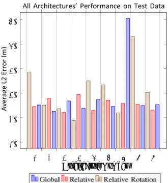
To compare each model’s efficacy, its estimated global

position for each image pair was compared to the ground truth and the Euclidian distances (L2 error) were summed. The average L2 error for each model during test sequences was typically between 200 and 400 meters (Figure 1). This differs greatly from the average losses during training sequences that are seen in Figure 2. For the Global and Relative models, the loss varied between 3-10 times less for known environments than it did for the test sequences. Figure 3 shows that the L2 error was dramatically larger for the Relative Rotation models than was the case for the other two model types and those models appeared to be far more sensitive to architecture changes. Similarly, the paths generated by Relative Rotational models were very often erratic. The paths predicted by the Global models tended to conform to the shape of the ground truth more often than other types.

Out of all the sequences that were tested, none of the models of any architecture performed well in unknown environments. Figure 1 demonstrates how the differences in L2 error between model performance in unknown environments were too low to gauge the relative superiority of any of the three models.

5. Conclusion

In this paper, the application of simple CNN architectures to the task of visual odometry was explored. It has been demonstrated that the CNN architectures detailed in this work are not well-suited for the task of visual odometry in unknown environments, but the Global and Relative models are able to correlate images and translation data in known environments with limited success. Separating the models into three core architectures and evaluating each with the same hyperparameters allowed for three unique approaches related to visual odometry. Most Global models could predict general trends in global position with limited success, and Relative models often performed near the same level as Global models. This is to be expected, as the DeepVO paper had presented similar results for their architectures [1]. None of the variants of Relative Rotation models achieved decent performance on the visual odometry dataset.

Architecture Number

Figure 1. Performance evaluation of generated architectures on test data.

6. Future Works

Results of this paper demonstrate the need for a fundamentally different architecture when attempting visual odometry versus standard classification. Other works suggest Siamese networks, in which multiple layers are used to extract features from each image individually, are better suited to visual odometry related tasks [6], [4]. Starting with a Siamese network and applying modern techniques such as Batch Normalization and Snapshot Ensembles will likely improve results dramatically from what is possible with the architectures used in this paper [4], [24], [25], [26]. Lastly, it is worth mentioning that, as suggested in [1], recurrent networks may be better suited to visual odometry than using a CNN architecture alone. 9 8 7 6 5 4 3 2 1 10 0 20 0 30 0 40 0 50 0 60 0 5 Graves et al.: Visual Odometry using Convolutional Neural Networks

(8)

References

[1] V. Mohanty, S. Agrawal, S. Datta, A. Ghosh, V. D. Sharma, and D.

Chakravarty, “Deepvo: A deep learning approach for monocular visual odometry.” 2016.

[2] C. Szegedy, W. Liu, Y. Jia, P. Sermanet, S. Reed, D. Anguelov, D.

Erhan, V. Vanhoucke, and A. Rabinovich, “Going deeper with convolutions.” 2014.

[3] A. Krizhevsky, I. Sutskever, and G. E. Hinton, “Imagenet classification with deep convolutional neural networks,” in Advances in Neural Information Processing Systems 25, F. Pereira, C. J. C. Burges, L. Bottou, and K. Q. Weinberger, Eds. Curran Associates, Inc., 2012, pp. 1097–1105.

[4] P. Agrawal, J. Carreira, and J. Malik, “Learning to see by moving,” CoRR, vol. abs/1505.01596, 2015. [Online]. Available: http://arxiv.org/abs/1505.01596

[5] P. Fischer, A. Dosovitskiy, E. Ilg, P. Hausser, C. Hazirbas, V. Golkov,¨

P. van der Smagt, D. Cremers, and T. Brox, “Flownet: Learning optical flow with convolutional networks,” CoRR, vol. abs/1504.06852, 2015. [Online]. Available: http://arxiv.org/abs/1504.06852

[6] E. Ilg, N. Mayer, T. Saikia, M. Keuper, A. Dosovitskiy, and T. Brox,

“Flownet 2.0: Evolution of optical flow estimation with deep networks,” CoRR, vol. abs/1612.01925, 2016. [Online]. Available: http://arxiv.org/abs/1612.01925

[7] C. Forster, Z. Zhang, M. Gassner, M. Werlberger, and D. Scaramuzza,

“Svo: Semidirect visual odometry for monocular and multicamera systems.” IEEE Transactions on Robotics, 2016.

[8] R. Mur-Artal and J. D. Tardos, “ORB-SLAM2: an open-source SLAM´ system for monocular, stereo and RGB-D cameras,” arXiv preprint arXiv:1610.06475, 2016.

[9] M. J. M. M. Mur-Artal, Raul and J. D. Tard´ os, “ORB-SLAM: a´

versatile and accurate monocular SLAM system,” IEEE Transactions on Robotics, vol. 31, no. 5, pp. 1147–1163, 2015.

[10] A. Geiger, P. Lenz, and R. Urtasun, “Are we ready for autonomous driving? the kitti vision benchmark suite,” in Conference on Computer Vision and Pattern Recognition (CVPR), 2012.

[11] “Robust monocular visual odometry using optical flows for mobile robots.” 2016 35th Chinese Control Conference (CCC), Control Conference (CCC), 2016 35th Chinese, p. 6003, 2016.

[12] “Semi-dense visual odometry for ar on a smartphone.” 2014 IEEE International Symposium on Mixed and Augmented Reality (ISMAR),

Mixed and Augmented Reality (ISMAR), 2014 IEEE International Symposium on, p. 145, 2014.

[13] A. Krizhevsky, “Learning multiple layers of features from tiny images,” Tech. Rep., 2009.

[14] C. Farabet, B. Martini, P. Akselrod, S. Talay, Y. LeCun, and E.

Culurciello, “Hardware accelerated convolutional neural networks for

synthetic vision systems,” in Proceedings of 2010 IEEE International Symposium on Circuits and Systems, May 2010, pp. 257–260.

[15] J. Bergstra and Y. Bengio, “Random search for hyper-parameter

optimization.” Journal of Machine Learning Research, vol. 13, pp. 281–305, 2012.

[16] E. Rosten, R. Porter, and T. Drummond, “Faster and better: a machine learning approach to corner detection.” 2008.

[17] F. Chollet, “Keras,” https://github.com/fchollet/keras, 2015.

[18] M. Abadi, A. Agarwal, P. Barham, E. Brevdo, Z. Chen, C. Citro, G. S. Corrado, A. Davis, J. Dean, M. Devin, S. Ghemawat, I. Goodfellow, A. Harp, G. Irving, M. Isard, Y. Jia, R. Jozefowicz, L. Kaiser, M. Kudlur, J. Levenberg, D. Mane, R. Monga, S. Moore, D. Murray,´ C. Olah, M. Schuster, J. Shlens, B. Steiner, I. Sutskever, K. Talwar, P. Tucker, V. Vanhoucke, V. Vasudevan, F. Viegas, O. Vinyals,´ P. Warden, M. Wattenberg, M. Wicke, Y. Yu, and X. Zheng,

“TensorFlow: Large-scale machine learning on heterogeneous

systems,” 2015, software available from tensorflow.org. [Online]. Available: http://tensorflow.org/

[19] J. D. Hunter, “Matplotlib: A 2d graphics environment,” Computing In Science & Engineering, vol. 9, no. 3, pp. 90–95, 2007.

[20] “The numpy array: A structure for efficient numerical computation.” Computing in Science & Engineering, Comput. Sci. Eng, no. 2, p. 22, 2011.

[21] M. Boyle, “quaternion: Add built-in support for quaternions to

numpy,” 2017. [Online]. Available:

https://github.com/moble/quaternion

[22] L. Clement, “pykitti: Python tools for working with kitti data,” 2016.

[Online]. Available: https://github.com/utiasSTARS/pykitti

[23] D. Kingma and J. Ba, “Adam: A method for stochastic optimization.”

2014.

[24] S. Ioffe and C. Szegedy, “Batch normalization: Accelerating deep

network training by reducing internal covariate shift.” 2015.

[25] G. Huang, Y. Li, and G. Pleiss, “Snapshot ensembles: Train 1, get m for free,” International Conference on Learning Representations, 2017.

[26] T. G. Dietterich, Ensemble Methods in Machine Learning. Berlin, Heidelberg: Springer Berlin Heidelberg, 2000, pp. 1–15.

(9)

All Architectures’ Performance on Training Data

Figure 2. Evaluation of performance of all generated architectures on training data.

Figure 3. The trajectories of Architecture 1

9 8 7 6 5 4 3 2 1 0 1,000 2,000 3,000 4,000 7 Graves et al.: Visual Odometry using Convolutional Neural Networks

(10)

Figure 4. The training loss (blue) and validation loss (orange) of Architecture 1

Figure 5. All paths of Architecture 4 along the xz-plane (in meters). Blue represents ground truth paths, orange represents Global model paths, red represents Relative model paths, and green represents Relative Rotation model paths.