Enhanced diversification by using unbundled returns

Enhanced diversification by using

unbundled returns

An analysis of an international multi asset

portfolio

Ytzen van der Werf

Fred Huibers

2013-04 February 2013

ASRE research papers ISSN 1878-4607

ASRE Research Center | Amsterdam School of Real Estate | Postbus 140 | 1000 AC Amsterdam | T 020 – 668 1129 | F 020 – 668 0361 | [email protected]

Enhanced diversification by using

unbundled returns

An analysis of an international multi asset

portfolio

Ytzen van der Werf Fred Huibers

Table of Contents

Executive Summary

3

1

Introduction

4

1.1 Recovery Plans of Pension Funds 4

1.2 Unbundled returns 5

1.3 The market for unbundled returns 6

1.3.1 Bonds 6

1.3.2 Stocks 6

1.3.3 Property 7

2

Methodology

8

2.1 Currency 9

2.2 Weights of the world indices 10

3

Data description

11

4

Results

14

4.1 Annual returns 15

5

Conclusion

18

Executive Summary

Dutch pension funds have been confronted with low coverage ratios since the economic crisis in 2008. In many cases their liabilities have outgrown their assets. This effect is partially caused by the negative total returns on stocks and real estate since the collapse of Lehman Brothers. Risk averse investors, for instance pension funds with relatively high aged participants, are increasingly exploring low risk investment strategies.

Previous research has shown that unbundling of total returns in their two components, income return and capital gains, decreases portfolio risk for real estate only portfolios. We believe unbundling of returns of all traditional asset classes (stocks, bonds and real estate) could provide enhanced diversification potential for international multi asset portfolios.

By analyzing these unbundled returns over a 10 year period we find that unbundling returns provide substantial risk reduction potential without losing any expected return. Simultaneously we find higher returns at similar levels of risk when unbundled returns are included in the asset mix. Finally we find that property income return is a major contributor to this diversification effect.

Although the market for property derivatives is only emerging we believe that unbundling returns could provide enhanced diversification opportunities. Furthermore such a market could provide valuable information about “the current fundamentals of the market”.

1

Introduction

1.1 Recovery Plans of Pension Funds

Meagre investment returns since 2007 in combination with historically low interest rates and the growing life expectancy have resulted in an asset-liability mismatch (“dekkingsgraad”) for many Dutch pension funds. These coverage ratios are important for Defined Benefit (DB) plans and since the Dutch DB plans account for 94% of all Dutch pension assets, its significance is large (Towers Watson, 2013).

In the end of 2007, nearly all Dutch Pension Funds showed coverage ratios above 105% and 65% even had coverage ratios of more than 130% (De Nederlandse Bank, 2012). One year later, 292 out of 409 funds saw their coverage ratio drop below 105%. When coverage ratios fall below 105%, pension funds need to draft recovery plans (“herstelplannen”) and provide them to De Nederlandse Bank (DNB). These recovery plans state how these pension funds will improve their financial position. There are three ways to improve the financial position:

1. no or lower price compensation for existing pensions; 2. raise premiums paid by current participants;

3. lower future pension payments.

Option 3. is generally considered the ultimate measure and will only be implemented when the other measures prove to have insufficient effect. Next April will be the first time in history that some of the largest Dutch Pension Funds (ABP, PME and PMT) will cut the pension rights by respectively 0.5%, 5.1% and 6.3% (IPE, 2013).

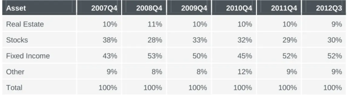
Also, DNB often requests pension funds to decrease their portfolio risk. Table 1 shows that pension funds have indeed altered their investment allocation significantly after the collapse of Lehman Brothers in 2008, and have maintained the lower risk profile up to today.

Table 1. Asset allocation Dutch Pension Funds

Asset 2007Q4 2008Q4 2009Q4 2010Q4 2011Q4 2012Q3 Real Estate 10% 11% 10% 10% 10% 9% Stocks 38% 28% 33% 32% 29% 30% Fixed Income 43% 53% 50% 45% 52% 52% Other 9% 8% 8% 12% 9% 9% Total 100% 100% 100% 100% 100% 100% Source: DNB (2013)

Table 1 shows that pension funds have raised the allocations to fixed income at the expense of stocks after the financial crisis set in and - by the end of 2012 - they have not reversed this decision. However, high grade fixed income assets generate low returns and this could prove to be a detractor to the speed with which recovery plans are realized. Based on previous research, we posit that unbundling the return of

traditional asset classes (stocks, bonds and real estate) in income return and capital gains allows pension funds to maintain the desired low risk profile while generating a return that is superior to that of the current asset mix.

1.2 Unbundled returns

The returns of traditional asset classes such as stocks, bonds and real estate consist of two components: direct returns, taking the form of dividend payments for stocks, coupon payments for bonds and net rent for real estate on the one hand and indirect returns measured as the changes in the price of the underlying asset on the other hand. Direct returns are (usually) cash flows that can be used to meet short term liabilities or can be re-invested and indirect returns are generated if and when assets are sold. However, the investment industry regards both components as equivalent and bundled since total return, used to determine asset allocation, is defined as the indivisible sum of (direct) income returns and (indirect) capital gain. This paper distinguishes between the two types of return and aims to determine whether the unbundled returns provide more diversification potential than total returns for investors with a global mandate. The authors expect property income return to act as a superior diversifier than the equity and bond counterparts since property usually shows higher direct returns that are relatively stable over time.

Adair et al. (2006) show for the UK that a split in income return and capital gains components favourably changes the allocation to the asset class real estate, especially in low risk portfolios. When total returns are observed, Direct Real Estate has a 24% and 55% allocation in respectively low and medium risk portfolios. These percentages are 81% and 41% if only the income component of all three asset classes is examined. Surprisingly, in higher risk portfolios income return on gilts seems to be a better asset. When only capital gains are considered, common stocks are the favoured asset in high risk portfolios, and real estate enters the low risk portfolio again with a 67% allocation.

In an unpublished dissertation, Van der Werf (2012) shows the different characteristics of the two return components for real estate in all 23 countries covered by the IPD. He finds that the correlation of domestic total returns with foreign income returns is on average .69 lower than the correlation between total returns mutually. This implies that an investor could better acquire foreign income return than total returns to diversify his domestic real estate portfolio.

McGreal et al. (2006) study the characteristics of income return and their allocations in a real estate only portfolio of Irish and UK property. Their analysis shows significantly different risk and return levels for the two components. As expected, income return is a low risk ‘asset’, where the capital gain is much more volatile and therefore riskier. Income returns and capital gains are treated as assets with income streams that could be purchased separately. McGreal et al. (2006, p. 139) suggest that this could easily be done with some minor financial engineering.

Bracke and Schmitz (2011) examine the risk sharing potential of investment income and capital gains on equities and their evidence suggests that international capital gains are a more potent channel of risk sharing. They tend to behave counter cyclically relative to the growth of local GDP.

1.3 The market for unbundled returns

1.3.1 Bonds

Stripping returns from bonds has existed for a certain period of time. In the 1960s a market for stripped bonds emerged. Stripped bonds are often called STRIPS, which stands for Separate Trading of Registered Interest and Principal Securities. The market for Strips flourished in the 80s after a tax omission in the US law. When bond coupons are treated differently from a tax perspective in different countries, arbitrage opportunities emerge as a result of those different tax treatments. The loophole was quickly closed but the stripped bonds remained in demand because of their simplicity.

1.3.2 Stocks

At the end of the last century Brennan (1998) foresaw the creation of a market for dividend strips, necessary for various reasons. First he thought such a market would provide valuable information about what he called “the current fundamentals of the market”, since equity markets should reflect the growth rate of dividends, which is an important input in stock prices. He argues that stock prices should reflect the discounted value of future cash flows measured by dividends. Secondly he felt there is no reason why strips should not be traded as there are always parties more interested in current dividends while others might be interested in future dividends, or the capital value change. Brennan proved to be right since by the end of 2008 around EUR 1bn worth of index dividend swaps are changing hands every day in the over-the-counter market, either to hedge dividend exposure or to benefit from arbitrage opportunities related to dividend performance (EUREX, 2008).

The dividend swap transaction is a very straight forward transaction between two investors and began as an over-the-counter (OTC) market. See figure 1 for a description of how it works.

Figure 1 | Dividend swap transaction

Source: Goldman Sachs research paper (2006), from Barakat and Coscas (2009)

Buyer Seller

Fixed amount of money Realized Dividends

1.3.3 Property

Although McGreal (2006) suggests that income return and capital gains could be created as separate assets with some minor financial engineering we notice that these financial products do not yet exist in the real estate investment industry.

The property derivative market is best established in the UK where the IPD UK all property annual total return swaps are being traded since 2004 and the trade volume peaked at a level of 11.8bn GBP outstanding contracts in the period before the fall of Lehman Brothers (IPD, 2013). Property swaps are being traded at minimum contract values of 50,000 GBP. In this exchange market, one party swaps its real estate total returns with a notional fixed rate, usually being the expected mean of future total returns. This is comparable to the dividend swap portrayed in figure 1.

However, as far as we are aware, no market exists for unbundled return swaps or other derivatives based on unbundled returns, although the IPD publishes unbundled returns for some markets on a periodic basis. On the other hand there is no fundamental reason why such a market could not exist or start to exist in the near future. As Brennan (1998) argued it could provide valuable information about the current fundamentals of the property market since property markets should reflect the growth of net rent and future yield shift.

2

Methodology

To analyse the effect of including unbundled returns in a Multi Asset Portfolio on an international scale we apply a Markowitz (1952) mean-variance optimization over a 10 year period. We construct world indices of returns in local currency for the three most common asset classes; stocks, bonds and real estate. By constructing world indices we are not focusing on the regional allocation of funds within an asset class, but instead we focus on asset classes themselves. To enable a useful comparison between the three asset classes we construct the world indices on a comparables basis. Thereto we have analysed the methodology used by the IPD to derive the different (unbundled) returns:

Income return Property:

∏ ( )

Where,

IRy = yearly income return

IRm = monthly income return

Capital gains Property:

∏ ( ) Where,

Outlayt= Investments in the property during a certain month

= Capital Value at month t

Total returns Property:

The last equation holds on a monthly basis. However, since annual returns have to be computed through compounding, this equation does not necessarily hold on an annual basis. To calculate annual returns the IPD uses the following formula:

∏ ( )

To calculate annual returns for stocks and bonds, the same methodology was applied by the authors with the only exception that we derived monthly total return (TR) and monthly capital gains (CG) from the Price and Return Indices provided by Datastream and computed monthly income return (IR) by subtracting CG from TR. In formulas:

Total return Stocks and Bonds:

∏( )

Where, RI = Return Index as provided by Datastream and t = end of the month and t-1 = beginning of the month

Capital gain Stocks and Bonds:

∏( ) Where, PI = Price Index as provided by Datastream

Income return Stocks and Bonds:

∏( )

Since we are specifically interested to see whether Property (total returns, capital gains or income return) has different risk-return characteristics than income return from stocks and bonds, we chose to construct a world index of these three asset classes. This way we are not examining whether it is more useful to invest in a specific region, but rather if real estate has different risk adjusted returns or diversification potential than stocks and bonds.

To construct the world index we chose an annually adjusted, equally weighted distribution over 4 regions; UK, US, Eurozone and Australia. These regions cover a substantial part of the world.

2.1 Currency

We have used returns in their local currency, USD for the US, GBP for the UK, EUR for the Eurozone and ASD for Australia. By using returns in local currency we focus on the actual returns of the underlying assets instead of their sensitivity for international trade and governments spending stability. However we are aware of the risk of exchange volatility and made an effort to control for exchange rate fluctuation. To compute either

unhedged or hedged returns in a single currency – USD, GBP, EUR or ASD – we needed the monthly IPD returns to calculate monthly returns in a single currency. Unfortunately IPD does not provide those returns in the Multi National Index Spreadsheet (IPD, 2011), therefore we were not able to control for currency risk.

2.2 Weights of the world indices

To construct the world indices for the asset classes we have used an equally weighted average of the yearly total and unbundled returns of all three asset classes. This implies a yearly rebalancing of the distribution within each asset type over the four regions considered. For instance, within Property we start year 1 with a 25% allocation to each region. At the end of year 1 there will be a different allocation due to different value changes. These differences will be neutralized by selling or buying those regions that are over- or underrepresented in such way that each region represents 25% again.

Another, and perhaps more realistic, method of constructing world indices would be a distribution based on market capitalisation. We have considered this but found the market capitalization for the bonds to be too unstable when compared to stocks and real estate (see figure 2).

Figure 2 | Relative market capitalisation of Bond indices over period of analysis

This is mainly caused by the fact that the index of 10 year government bonds is created by the available series of government bonds with a maturity of nearly 10 years. As a result, since the maturity of a single series decreases over time, and new series can be brought on the market, the capital value of these bond indices changed significantly. Therefore we decided not to use this method of constructing world indices. As a result Australia plays a rather large part in our analysis but a quick check shows similar results for world indices based on the weighted average based on market caps.

0% 10% 20% 30% 40% 50% 60% 70% 80% 90% 100% 2001 2002 2003 2004 2005 2006 2007 2008 2009 2010

Relative market cap Bonds

AUS UK US EUR

3

Data description

To determine the effect of unbundled returns in an international Multi Asset Portfolio context indices for stocks, bonds and real estate from 4 regions across the globe are selected. The four regions considered are Eurozone, UK, US and Australia. Table 2 shows the Indices used as representative for the different asset classes.

Table 2 | Indices used for Stocks, Bonds and Real Estate

Asset Country Series Provider Years of data

Stocks EURO EUROS STOXX (297 constituents) Dow Jones 25 US S&P 500 Composite S&P 48

UK FTSE100 FTSE 35

AUS S&P-ASX-300 S&P 15 Bonds EURO EMU Benchmark Gov. 10 Years 13 US US Benchmark Gov.10 Years 23 UK UK Benchmark Gov.10 Years 23 AUS AUS Benchmark Gov.10 Years 23 Real Estate EURO TR, IR, CG IPD 10

US TR, IR, CG IPD 10

UK TR, IR, CG IPD 10

AUS TR, IR, CG IPD 10

Since the IPD has the shortest period of data available, we consider a 10 year period ranging from 2001-2010. By the end of 2010 these four regions represent 70% of the market value of all property markets covered by the Investment Property Databank (IPD, 2011). The IPD provides annual total returns in local currency, which are unbundled in their respective annual direct and indirect returns. However, IPD calculates these annual property returns from returns collected on a monthly basis.

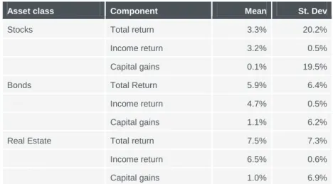
Table 3 shows the mean returns and standard deviations of the unbundled returns of the world indices and table 4 shows their correlations.

Table 3 | Average annualized mean and standard deviation of total returns and unbundled returns of different asset classes

Asset class Component Mean St. Dev

Stocks Total return 3.3% 20.2% Income return 3.2% 0.5% Capital gains 0.1% 19.5% Bonds Total Return 5.9% 6.4% Income return 4.7% 0.5% Capital gains 1.1% 6.2% Real Estate Total return 7.5% 7.3% Income return 6.5% 0.6% Capital gains 1.0% 6.9%

Table 3 shows the very low risk (measured as standard deviation) of income returns, either stocks, bonds or property. It also indicates that real estate income returns seem to have the most favourable risk-return characteristics exhibiting a 6.5% return with a 0.6% risk. To be able to conclude that real estate income return will enter the efficient frontier portfolio, the correlation with other assets should be analysed, since Markowitz (1952) argues it is mainly the low to negative correlation with other assets that effectively lowers the risk of the portfolio.

Table 4 | Correlation between asset classes

Correlation STR SIR SCG BTR BIR BCG PTR PIR PCG

Stocks TR 1,00 Stocks IR 0,22 1,00 Stocks CG 1,00 0,20 1,00 Bonds TR -0,87 -0,02 -0,87 1,00 Bonds IR -0,35 -0,95 -0,33 0,17 1,00 Bonds CG -0,85 0,03 -0,86 1,00 0,12 1,00 Property TR 0,43 -0,60 0,45 -0,29 0,48 -0,31 1,00 Property IR 0,05 -0,42 0,06 -0,22 0,44 -0,25 0,09 1,00 Property CG 0,43 -0,57 0,44 -0,27 0,45 -0,30 1,00 0,01 1,00

Table 4 shows low to highly negative correlation (in red) between all return components of bonds and all return components from stocks, varying from .03 to -.95. Bond total returns (and capital gains) are negatively correlated with all the property returns, varying from -.22 to -.31.

However, stocks total return (and capital gains) have a low to medium positive relationships with all property components (.05 to .45).

Based on the correlations expressed in table 4 one would expect bonds to enter the minimum variance optimal portfolio with either a mix of property or stocks to create higher returns. Markowitz’ (1952) mean variance optimization combines the data given in tables 3 and 4 to calculate the optimal allocation framework.

4

Results

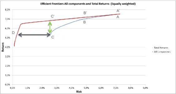
Applying the Markowitz (1952) mean variance optimization procedure on the unbundled returns of the world indices of stocks, bonds and direct real estate, we find that unbundling returns enhances the diversification potential of the mixed asset portfolio. Figure 3 shows the efficient frontiers of two portfolios. One portfolio with only total returns, which we will refer to as Total Return Portfolio (blue line) versus the efficient frontier considering total returns, income returns and capital gains. This portfolio will be called All Components portfolio (red line).

Figure 3 | Efficient frontiers of Total Returns versus All Components

When ‘high risk’ portfolios are analysed we find no difference between the expected return of the Total Return and the All Component portfolios (A versus A’). The difference in expected returns at 7.3% risk is null, since both portfolios are nearly only Property Total Returns (see table 4 and 5). At medium level risk of 4.9% we find a difference of .2% in expected return in the advantage of the All Components portfolio. At the minimum risk level of the Total Return portfolio (point C) the difference in expected return has risen to 1.4% which means the return of the All Component portfolio is nearly 27% higher than the expected return of the minimum variance Total Return portfolio (green arrow).

However, at the same level of return (5.4%) the risk of the all component portfolio will decrease to 0.3% (point D), which we have defined as ultra-low risk. This is a 90% decrease of the portfolio risk (black arrow).

Next we analysed the distribution of the portfolios over the different asset classes. First we examined the Total Return portfolio at different levels of risk (table 4). At the point of minimum variance (risk 2.6%) bonds cover nearly three quarters of the portfolio, followed by stocks (21%) and property with only 4.6%. The share of real estate increases rapidly when medium risk portfolio strategies are considered and the high risk portfolio contains nearly only property total returns.

A D A’ B’ B C C’

Table 4 | Asset allocations Total Return portfolio

Risk appetite Risk Return Stocks Bonds Real Estate

Low risk 2.6% 5.4% 21.1% 74.3% 4.6%

Medium risk 4.9% 7.0% 31.0% 69.0%

High Risk 7.3% 7.5% 0.1% 99.9%

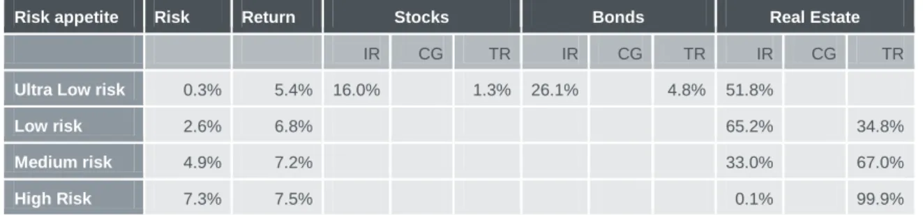
When unbundled returns are included in the analysis the allocations shift significantly (see table 5). Since including the unbundled returns in the analysis lowers the risk of the minimum variance portfolio we introduced an ultra-low risk portfolio to be able to compare the other allocations to the total return Portfolio at the same levels of risk but also displaying the allocation when the risk level is very low.

Table 5 | Asset allocation All Component portfolio

Risk appetite Risk Return Stocks Bonds Real Estate

IR CG TR IR CG TR IR CG TR

Ultra Low risk 0.3% 5.4% 16.0% 1.3% 26.1% 4.8% 51.8%

Low risk 2.6% 6.8% 65.2% 34.8%

Medium risk 4.9% 7.2% 33.0% 67.0%

High Risk 7.3% 7.5% 0.1% 99.9%

At the ultra-low level of risk, allocations 16% should be made to stocks income returns. Stocks disappear from the optimal portfolio when risk increases to low, medium or high levels. At the low risk level (2.6%) the portfolio exists only of real estate income or total returns. Property total return is included because of its higher returns. At the highest risk level the portfolio allocation does not differ from the Total Return portfolio anymore since the highest return comes from property total returns only.

We find that income returns enhance the diversification potential of a Multi Asset Portfolio significantly since income returns from either stocks, bonds or real estate cover nearly 94% of the minimum variance portfolio. Furthermore property, and more specifically property income return play a significant role in the All Component portfolio at the low risk level when compared to the total return portfolio, where 75% of the portfolio is allocated to bonds. Capital gains from either stocks, bonds or real estate do not provide any enhanced diversification potential.

4.1 Annual returns

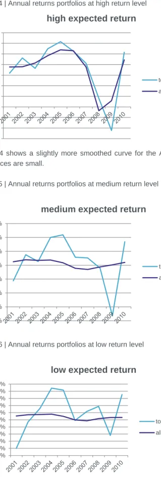
Table 4 and 5 show that mean returns are higher when unbundled returns are added to the international Multi Asset Portfolio. However, the most important finding of our research is the possibility to minimize risk at similar levels of return within an All Component portfolio. To illustrate this finding we present figures 4, 5 and 6 which display the annual average returns at three levels of mean expected return. We chose a high return level of 7.0%, medium level of return (6.2%) and a low level of return of 5.4%. So, both portfolios exhibit the same mean expected return but different volatility.

Figure 4 | Annual returns portfolios at high return level

Figure 4 shows a slightly more smoothed curve for the All Components portfolio, but differences are small.

Figure 5 | Annual returns portfolios at medium return level

Figure 6 | Annual returns portfolios at low return level -6,0% -4,0% -2,0% 0,0% 2,0% 4,0% 6,0% 8,0% 10,0% 12,0% 14,0%

high expected return

total returns all components -2,0% 0,0% 2,0% 4,0% 6,0% 8,0% 10,0% 12,0%

medium expected return

total returns all components 0,0% 1,0% 2,0% 3,0% 4,0% 5,0% 6,0% 7,0% 8,0% 9,0% 10,0%

low expected return

total returns all components

Figure 5 and 6 however clearly show much smaller volatility of the annual returns when unbundled returns could be included in the asset mix. Furthermore including unbundled returns at the lower levels of expected return, a lower risk investment strategy applied by most of the pension funds with an older population or a large proportion of retirees does not display negative or even low annual returns anymore. This could result in a much more stable course of the Asset-Liability ratio and therefore a smaller chance of falling below the desired 105% threshold for coverage ratios. At least as far as the asset side of the equation is being considered. We are aware of the fact that our findings do not have an impact on the liability side of the possible mismatch.

5

Conclusion

By using unbundled returns instead of using only total returns of traditional asset classes, investors could achieve a significant improvement of the risk/return characteristics of their global investment portfolio. This effect is particularly pronounced in the lower risk territory where we find a 90% decrease of portfolio risk could be achieved. The relatively stable and high returns of the income component of real estate investments are the main contributor to this positive effect.

This result enhances the possibilities for institutional investors that are restricted to this lower risk territory. A current example are Dutch pension funds that have to improve their coverage ratio. At the long term, growing longevity and a higher dependency ratio implies that the lower risk territory is likely to become more important. Furthermore, more and more of the pension funds are considering shifts from Defined Benefit to Defined Contribution. This implies that larger parts of new employees will enter the DC plans and as a result the average age of the participants in DB plans will grow and therefore risk should be reduced.

This paper suggests that creating a market for unbundled real estate returns would be very helpful for investors to improve the risk/return characteristics of their portfolio, since without these markets there is no opportunity to include unbundled returns. Furthermore unbundling returns could provide valuable information about what Brennan (1998) called “the current fundamentals of the market”, since real estate investment markets should reflect the growth rate of net rent.

The growing demand from institutional investors will stimulate supply of cost efficient provision of unbundled returns. While this market is gradually developing, it is likely to accelerate in the coming years.

Literature

Adair, A., McGreal, S. and Webb, J. (2006) Diversification effects of direct versus indirect real estate investments in the UK. In: Journal of Real Estate and Property Management May 2006 pp. 85-90.

Barakat, H. and Coscas, J. (2009) Listed dividend swaps on Eurex: Does mispricing mean arbitrage opportunities. Final year Thesis HEC Paris May 2009.

Bracke, T. and Schmitz, M. (2011) Channels of international risk-sharing, capital gains versus income flows. In: International Economics & Economic Policy, vol 8. no 1. pp. 45-78.

Brennan, M. (1998) Stripping the S&P 500 Index. Financial Analysts Journal, January/February 1998 vol. 54 no. 1 pp. 12-22

De Nederlandse Bank (2013) T8.8 Geraamde dekkingsgraad van pensioenfondsen. From:

http://www.statistics.dnb.nl/financieele-instellingen/pensioenfondsen/toezichtgegevens-pensioenfondsen/index.jspRetrieved at 5 February 2013

EUREX (2008) Xpand December 2008 From: http://www.eurexchange.com/blob/exchange-en/3066-3100/115552/2/data/e_xpand_2008127.pdf.pdfRetrieved at 12 February 2013

Goldman Sachs (2006) US portfolio strategy – Turning cash into value. From: www2.goldmansachs.com/ideas/portfolio-strategy/us-portfolio-turning-cash-pdf.pdf Retrieved at 12 December 2012

Investment Property Databank (2011) IPD Multinational Index Spreadsheet, Global Index Performance (2010 update 6) [online]

Investment Property Databank (2013) IPD/IPF Trade Volume Report UK, From

http://www.ipd.com/Portals/1/Derivatives%202013/Q4%202012%20Derivates%20trading%20vo

lumes%20UK.pdf Retrieved at 12 February 2013

IPNederland (2013) Kortende pensioenfondsen bekend. From: http://www.ipe.com/nederland/

kortende-pensioenfondsen-bekend_50159.php Retrieved on 19 February 2013

Markowitz, H. (1952) Portfolio Selection. In: Journal of Finance, vol 7 no. 1 pp. 77-91

McGreal, S., Adair, A., Berry, J. and Webb, J. (2006) Institutional real estate portfolio diversi-fication in Ireland and UK. In: Journal of Property Investment Finance vol. 24 no. 2, pp. 136-149

Towers Watson (2013) Global Pension Asset Study 2013. From: http://www.towerswatson.com/

assets/pdf/8991/Global-Pensions-Asset-Study-2013-Towers-Watson.pdf January 2013

Van der Werf, Y. (2012) Risk reduction via operating channels on direct Real Estate Investment.

Neem voor vragen of opmerkingen over onze opleidingen contact met ons op of bezoek onze website. bezoekadres Jollemanhof 5 1019 GW Amsterdam postadres Postbus 140 1000 AC Amsterdam www.asre.nl e [email protected] t 020 668 11 29 f 020 668 03 61

De activiteiten van de Amsterdam School of Real Estate zijn mede

mogelijk dankzij de financiële steun van de Stichting voor

Wetenschappelijk Onderwijs en Onderzoek in de Vastgoedkunde

(SWOOV)

Onze donateurs

I 3W Vastgoed BV I Aberdeen Asset Management I ACM Vastgoed Groep BV I Ahold Vastgoed BV I Altera Vastgoed I AM BV I AMVEST I ASR Vastgoed Ontwikkeling I ASR Vastgoed Vermogensbeheer I Ballast Nedam Ontwikkelings- maatschappij B.V. I Bemog Project-ontwikkeling B.V. I Boekel De Nerée NV I Bouwfonds Property Development I Bouwinvest I Brink Groep I CBRE Global Investors I Colliers International l Corio I De Brauw Blackstone Westbroek I Deloitte

I Delta Lloyd Vastgoed

I DTZ Zadelhoff I Dura Vermeer Groep NV

| ECORYS Nederland BV

I Ernst & Young Real Estate Group I FGH Bank NV I Funda NV | G&S Vastgoed I Haags Ontwikkelingsbedrijf | Heijmans Vastgoed I Houthoff Buruma I ING Real Estate Finance

I IPMMC Vastgoed I IVBN

I KMPG Accountants I Lexence NV I Loyens & Loeff NV | MAB Development I Mitros I MN I NSI I NS Vastgoed BV I NVM I Ontwikkelingsbedrijf Gemeente Amsterdam I Ontwikkelingsbedrijf Rotterdam I PGGM I Provast I PwC I Rechtstaete vastgoedadvocaten &belastingadviseurs BV I Redevco Europe Services BV I SADC I Savills Nederland BV I Schiphol Real Estate BV

I SNS Property Finance

I SPF Beheer BV I Strabo BV

I Syntrus Achmea Real Estate & Finance I TBI Holdings BV I The IBUS Company I Uni-Invest

l Van Wijnen Holding N.V. I Vesteda Groep BV I Volker Wessels Vastgoed I Wereldhave NV I WPM Groep I Yardi Systems BV I Ymere