TAX-BENEFIT MICROSIMULATION MODELS FOR THE EVALUATION OF PUBLIC POLICIES

(1)

Alma Mater Studiorum – Università di Bologna

DOTTORATO DI RICERCA ECONOMIA

CICLO XXII SECS-P/06, SECS-P/03

TAX-BENEFIT MICROSIMULATION MODELS FOR

THE EVALUATION OF PUBLIC POLICIES

Daniele Pacifico

Coordinatore Dottorato Relatore

Prof. Andrea Ichino Prof. Massimo Baldini

(2)

(3)

Part I.

(6)

(7)

1. Acknowledgements

I would like to thank everyone who contributed to make possible the research contained in this thesis.

I am deeply grateful to my supervisor Massimo Baldini who always encouraged me and facilitated my research with precious tips and suggestions.

Andrea Ichino and Luca Lambertini, the coordinators of the Ph.D. program in Economics at University of Bologna also never denied their support. Richard Blundell, Costas Meghir Monica Costa Dias provided important feedback during my research periods at the University College London, UK.

Besides the contribution of my supervisor, the material in this thesis has bene-fited of the comments of many colleagues, senior academics and friends.

Comments on Chapter 3 were provided by several members of the IFS staﬀ, in particular Monica Costa Dias and Mike Brewer and many colleagues as Miriam Hortas Rico and Alessia Russo.

Part of the material in Chapter 4 is related to an essay published in the journal "Rivista Italiana degli Economisti", which benefited of the comments of Paolo Bosi, Paolo Silvestri and an anonymous referee.

In writing Chapter 5, I benefited of the suggestions of Kenneth Train, Mike Brewer, Peter Haan and Monica Costa Dias. Part of the material included in the chapter was presented in several occasions, benefiting from several comments from the audience.

The support of the Ministero dell’Istruzione, dell’Università e della Ricerca, through the Ph.D. scholarship at University of Bologna is also gratefully acknowl-edged.

Finally, this thesis would not have been possible without the love of all my family - in particular of my mother, my father and my syster - and all my friends, in particular Maria Zindili, Francesco Zambelli and Sebastien Rippert.

(8)

(9)

2. Introduction

2.1. Static, dynamic and behavioural microsimulation

models for the analysis of public policies

Microsimulation models are a useful tool for the ex-ante evaluation of specific tax-benefit reforms. They are called micro-simulation models since, diﬀerently from typical macroeconomic models, they preserve individual heterogeneity in the simulation exercise.

The literature has proposed several types of microsimulation models. The most common ones are known as static models. Their aim is to simulate in a very precise way the national (and local) system of taxes and benefits using large microdata surveys that are representative of the whole population. In particular, they recover gross earnings (if not observed) and then simulate taxes amounts and benefit entitlements for each unit in the sample in order to get the observed individual net disposable incomes. These kind of simulators are useful for the evaluation of the distributive impact of specific tax-benefit reforms. Indeed, once the tax-benefit system changes, the vector of net disposable income that is recovered by means of the simulation model will be diﬀerent from the original one (which is computed according to the baseline tax-benefit system). Hence, the analyst can compute the income distribution before and after the change and identify winner and losers from the proposed reform.

These models are defined as “static” because they do not account for two im-portant dimensions: individual dynamics (what happens in period t+1?) and behaviour (what is the individual reaction to a specific change in the economic environment?). According to these two dimensions, the literature has proposed dynamic microsimulation models and behavioural microsimulation models. Impor-tantly, traditional dynamic microsimulation models do not account for behaviour in a structural way as a behavioural microsimulation model does. Indeed, they mainly work with transition probabilities (recovered from diﬀerent source of data)

(10)

and Markov processes so that a given event is not the result of an explicit optimal decision based on a structural microeconomic model.

As an example, assume a specific individual is observed working full time in period t. In period t+1, this individual will change his working time (say from full time to part-time) if, and only if, his/her specific transition probability - which is computed from a multivariate econometric model so that it depends on a set of observed individual characteristics - is higher then a random number drawn from a (typically uniform) probability distribution. The dynamic evolves in this way for many important events of the individual life, as fertility, marriage, child-bearing, education, health, disability, type of work, job eﬀort, retirement, mortality, etc. Hence, the analyst can forecast the distribution of a specific characteristic - say net disposable income - over a long time span so that the eﬀect of a specific reform today (as a pension reform) can be evaluated in the long run. The aim of behavioural microsimulation models, on the other hand, is to use the standard economic theory to predict specific changes in individual choices once a given element of the economic environment has changed.

As an example, assume the government introduces a new tax. Then, it is plausi-ble that some people will change their behaviour in the labour market, say reducing the number of hours they work from a full time to a part time contract. Accord-ing to this example, a behavioural microsimulation model uses a microeconomic model (typically with optimising behaviour subject to given budget constraints) to predict the overall change in the number of hours of work related to the change in the tax system. Of course, this behavioural change will take time to take place but the behavioural model do not consider the dynamic of this adjustment, it just gives the new final optimal choice. As these two examples have shown, behavioural and dynamic microsimulation models are intrinsically diﬀerent and cannot be com-pared. However, thanks to the progress in computer technology, a new generation of models known as structural dynamic microsimulation models will be soon op-erative and will allow exploring the dynamics of behavioural reactions to specific changes in the economic environment over the life cycle1_.

The literature has already proposed a dynamic simulation model for the Italian case2_{. As for Italian behavioural microsimulation models, the work of Aaberge}

et al. (1998) and Aaberge et al. (2000) is particularly important, since these authors

1_{For a recent example of such models see van de Ven and Weale (2009).} 2_{See Mazzaferro and Morciano (2008) for details.}

(11)

2.1. Static, dynamic and behavioural microsimulation models for the analysis of public policies

have been some of the first in the international literature to propose a specific framework for the analysis of simulated behavioural responses to tax reforms using microsimulation models. However, the literature has proposed another approach for behavioural microsimulation models, which is based on the work of Van Soest (1995) and Keane and Moﬃtt (1998). As we will see, the two approaches are similar and their main diﬀerence rests on the way the individual choice set is constructed.

The main aim of this dissertation is to propose a behavioural microsimulation model that explores and expands the Van Soest’s approach for the Italian case. In-deed, we propose a behavioural model that is able to account for many dimensions that are expected to influence the labour supply decision of many individuals. In particular, we allow for child-care expenditures, observed and unobserved individ-ual preference heterogeneity for consumption and leisure, fixed costs of working and joint labour supply for married couples. The model is applied to the evaluation of the distributive and efficiency effects of the last three main reforms of the Italian personal income tax and important conclusions about the equity-efficiency trade off are discussed and analysed. Furthermore, we explore in deep detail the practical implications of unobserved preference heterogeneity for consumption and leisure in discrete models of labour supply, which is of interest to any kind of behavioural microsimulation model, no matter the approach used. In particular, we claim that the way researchers account for unobserved tastes in the econometric specification has an important impact on the subsequent estimates, and this - in return - implies that the efficiency and welfare analysis may change significantly depending how unobserved heterogeneity is introduced in the specification. Of course, this has important implications for the empirical literature, the aim of which is to evaluate specific tax-benefit reforms in order to derive policy recommendations.

In general, we believe that behavioural models are a very powerful tool for the evaluation of public policies and this thesis contributes to this literature exploring specific issues and proposing an innovative model for the Italian case. Obviously, much more can be done and several lines for future research are proposed in several occasions throughout the various chapters.

(12)

2.2. Behavioural microsimulation models and structure of

this thesis

This thesis is dedicated to the analysis of behavioural microsimulation models for the evaluation of the eﬀects of specific tax-benefit reforms on the labour supply decisions of the Italian population. As we have anticipated in the previous section, a behavioural microsimulation model contains a structural microeconomic model that explains the link between the two phenomena under analysis, that is the tax-benefit roles and the labour supply decision, in our specific case. Of course, the results of any simulation depend on the specific model used in the analysis and its assumptions. Hence, great care will be devoted to the specification of our model and to the analysis of its implicit and explicit assumptions.

Chapter 3 contains a detailed explanation of the model we propose, with a special focus on the econometric framework used for both the estimation and identification of the structural parameters. In particular, we will explore the performance of a labour supply estimation method based on a discrete choice set. The idea behind this approach is to work directly with preferences for leisure and consumption, instead of typical labour supply functions.

As it will be clarified, the main advantage of the discrete approach is the pos-sibility to deal easily with non-convex budget sets, household labour supply and non-participation choices. Of course, these advantages let the discrete approach relatively suitable for policy evaluation purposes. We will use the papers from Blundell, Dancan, McCrae and Meghir (1999) and Brewer, Duncan, Shepard and Suarez (2006) as main references for the structural microeconometric model and several innovative elements will be taken into account with respect to previous Italian studies. In particular, we present a model that allows for errors in the pre-dicted wages for non-workers, unobserved heterogeneity in preferences, unobserved monetary fixed costs of working and child-care demand.

The chapter concludes presenting and disussing the labour supply elasticities for married women and men that we computed throughout our model. Finally, an overview of the Stata®_{routine for the Simulated Maximum Likelihood estimation}

is presented in the appendix.

Chapter 4 contains an application of our behavioural model to the evaluation of the distributive and eﬃciency eﬀects of the three most recent reforms of the Italian personal income tax. In order to show the functioning of our model, the analysis

(13)

2.2. Behavioural microsimulation models and structure of this thesis

of these reforms will be carried out in three different stages. In the first one we will study the “pure” distributive effects of the reforms using the static part of our microsimulation model. In the second stage we will focus on the labour supply effects by means of the structural microeconometric model of household labour supply outlined in the previous chapter; finally, we will analyse the distributive effects of the reforms accounting for labour supply reactions.

Our findings confirm that the extension of the no-tax area had positive eﬀects in terms of both redistribution and work incentives, and in the same time greater ben-efits for households with children improved income distribution but with negative eﬀects on the labour supply of married women.

Finally, chapter 5 focuses on the role of unobserved preference heterogeneity in structural discrete choice models of labour supply. Within this framework, unobserved heterogeneity has been estimated either parametrically or nonpara-metrically through random coefficient models. However, several examples in the literature have shown that the estimation of such models by means of standard, gradient-based methods is often difficult, in particular if the number of random parameters is high. For this reason, the role of unobserved tastes variability in empirical studies is constrained, since only a small set of coefficients is allowed to be random. However, this simplification may affect the estimated labour supply elasticities and the subsequent policy prescriptions.

Following this intuition, in this chapter we propose a new estimation method based on an EM algorithm that allows to fully consider the eﬀect of unobserved heterogeneity nonparametrically. Results show that labour supply elasticities and policy prescriptions do change significantly only when the full set of coeﬃcients is assumed to be random.

Moreover, we will analyse the behavioural eﬀects of the introduction of a working-tax credit scheme in the Italian working-tax-benefit system and show that the magnitude of labour supply reactions and the post-reform income distribution can diﬀer sig-nificantly depending on the specification of unobserved heterogeneity.

(14)

(15)

Part II.

Behavioural Microsimulation

modelling

(16)

(17)

3. A behavioural microsimulation model

for Italian married couples

(18)

3.1. Introduction

Discrete vs continuous structural labour supply models

Traditionally, structural labour supply models assume a choice set defined on any positive real number of worked hours. This is what Van Soest (1995) defines as the

continuous approach. In this continuous framework, the agent chooses the best combination of consumption and leisure so as to maximise her utility function given a time and a budget constraint. Importantly, there are no constraints on the amount of leisure the agent can choose from: hours of leisure can be any real number up to the maximum amount available.

The literature has developed two diﬀerent approaches for continuous labour supply. Often, a labour supply function is estimated relating hours worked with net-wage rates, non-labour incomes and individual characteristics. Then, indirect utility and expenditure functions are recovered by integration methods. Neverthe-less, appropriate constraints on the parameters have to be imposed a priory so as to ensure duality conditions to hold. Moreover, in order to capture a relative wide range of labour supply behaviour, a reasonably flexible labour supply function is needed, with the subsequent diﬃculties during the integration procedure.

Another possibility in continuous microsimulation is to work directly with pref-erences with supply function derived from either a direct or an indirect utility function. Here the main problem is the tax schedule that enter the budget con-straint, which can create several problems in the estimation stage.

In general, continuous microsimulation suﬀers of several problems no matter the approach followed. A first starting issue, for example, is how to recover the budget constraint for each possible level of labour supply. In continuous models, one or five minutes intervals of labour supply are needed for each individual, which means that with a standard total amount of time of 80 hours per week and thousands of individuals in the sample, this would be extremely time consuming1_.

Another complicated issue is the presence of a real tax-benefit system, which may give rise to highly non-linear and non-convex budget sets for most of the pop-ulation of interest. This implies that feasible estimations require the linearisation of the budget constraint around the observed level of hours or the construction of search algorithms that compare the maximum utility on each linear segment of a

1_{Duncan and Stark (2000) have developed an algorithm in GAUSS that is able to recover budget sets} more eﬃciently and accurately.

(19)

3.1. Introduction

piecewise-linear budget constraint2_.

Moreover, considerable problems arises because of the simultaneity between net-wages and hours of work with the subsequent necessity to find appropriate instru-ments so as to ensure identification. Finally, other diﬃculties arise when the model try to allow for important extensions like unobserved preference heterogeneity, joint labour supply and non-participation.

As Creedy and Duncan (2002) point out, these criticisms make the continuous approach seldom used nowadays. Indeed, the recent literature has shown that a discrete approach to labour supply modelling solves most of the problems that are typically found in continuous models and allows for some important extensions.

The discrete model of labour supply is still based on the assumption of utility maximising agents as in the continuous approach but now the agent is constrained to choose from just few hour points instead of any possible hour in the real line. The utility is defined over income and leisure (hours of work) and any assumption is made a priori on the marginal (dis)utility of leisure (work) and income. If a stochastic component is added to the utility function, then the probability of a particular choice of hours of work can be derived and the likelihood function can be computed. In other words, what is estimated in the discrete approach are not the parameters of a classical Marshallian labour supply function but the parameters that define the shape of the utility function.

Given that the tax-benefit system enters the utility only indirectly through the consumption term, complicated tax schedules and non-convex budget sets do not represent a problem anymore. Moreover, any problems arise from the choice of the utility function given that the form of the probabilities depends on the assumptions on the utility stochastic component. Finally, the budget constraints have to be computed for just the few hour points the agent is constrained to choose from, and not for any possible level. Furthermore, the discrete approach allows for important extensions that are diﬃcult to consider in the continuous model. Indeed, as it will be clarified later, wage unobserved components for non-workers, child-care demands, fixed costs of working, heterogeneity in preferences, non-participation and joint labour supply can be incorporated in the model in a very convenient way.

2_{A first generation of model linearized the budget constraint by computing the average net wage rate} corresponding to the observed hours. Other subsequent models have elaborated algorithms that examine the full budget constraint when searching for the optimal level of labour supply, allowing for nonlinearities and nonconvexities. See Creedy and Duncan (2002) for references.

(20)

The main drawbacks of the discrete approach are the rounding errors produced when the choice set is discretised and the incomplete use of available information3_.

As Blundell and MaCurdy (1999) point out in their literature review of labour supply modelling, the discrete approach has to be preferred to other models be-cause of its flexibility, in particular when the aim is the ex-ante evaluation of a specific policy reform. Modelling labour supply responses using a discrete approach has become increasingly popular in recent years, in particular when the aim of the analysis is the evaluation of a specific tax reform.

Earlier international works that explore this method are those from Van Soest (1995), Keane and Moffitt (1998) and Blundell et al. (2000). The econometric model used in these papers has now become standard in the literature and a similar version is also used in this work. Recent examples include: Brewer et al. (2006) who extend the paper of Blundell et al. (2000) to study the impact of the WFTC reforms in the UK, Breunig et al. 2008 who estimate the wage equation and the structural labour supply model simultaneously allowing for correlation between the random terms, Haan (2006), who studies the German case comparing the performance of a random coefficients specification with respect to the performance of a more simple model without unobserved heterogeneity, Labeaga et al. (2008) who study the impact of the Spanish tax reform on efficiency and social welfare. A very active centre that is specialised on microsimulation and labour supply in a discrete choice framework is at the Melbourne Institute of Applied Economics. I remand to Creedy and Kalb (2005) for a review of some of their papers.

For the Italian’s case Aaberge et al. (2000) developed a model of labour supply allowing for diﬀerent job types for each household; in their paper, job alternatives are defined over a continuum of wage rates, hours of work and other job character-istics. The analyst does not observe the opportunity set of each household so that the probability of choosing a particular job has to be weighted with the probability of receiving that particular job oﬀer. Recently, Mancini (2007), developed a model that is closely related to the one discussed here in order to study the labour supply response to minimum income policies. Del Boca et al. (2005) study the impact of child-care rationing on female labour supply using a bivariate probit model for the joint decision of child-care and labour supply.

However, diﬀerently from the other models that have been developed for the

3_{The wider the hours categories used to discretise the choice set the bigger the rounding error, see} Van Soest (1995) for this point.

(21)

3.1. Introduction

Italian case, the model presented in this paper accounts for many innovative fea-tures simultaneously. Indeed, we estimate jointly the labour supply behaviour of married women and men allowing for errors in predicted wages, work-related mon-etary costs, child-care costs and unobserved random preferences for consumption and leisure.

Work-related monetary costs are important since they eliminate the reservation wage condition in estimation and, depending on how these costs are specified, they may help to relax the assumption of fixed wage rates4_.

Furthermore, we also account for endogenous child-care expenditures and un-observed heterogeneity in preferences. Both these features are relevant. From a practical point of view, child-care expenditures have a role similar to those of other fixed costs of working since they may help to eliminate the reservation wage condi-tion for household with children during the estimacondi-tion. Unobserved heterogeneity is also important so as to get unbiased estimates given the assumption made on the distribution of the utility function5_.

Finally, one more important diﬀerence from previous studies regards the way we take into account the endogeneity related to estimated wages for non-workers. Indeed, we integrate out wages by drawing randomly from their estimated distri-bution and weighting the likelihood when wages are not observed in the data.

This chapter is structured as follows. Section 2 presents the general framework for the structural microeconometric model. Section 3 presents the extensions to the basic model. Section 4 explains the data used for the empirical analysis. Section 5 describes the estimation procedure. Section 6 contains results from first stage regressions and section 7 discusses the estimates of the structural model. The appendix contains an overview of the Stata® _{algorithm coded for the estimation}

of the structural model.

4_{See Brewer et al. (2006) for this point.}

5_{As it will be clarified later, the direct utility function is assumed to follow a type 1 extreme value} distribution, which underlines the typical IIA (independence from irrelevant alternatives) property. The way unobserved heterogeneity is introduced can relax the extent of this assumption and this is important because such property could be particularly binding in our labour supply framework.

(22)

3.2. The structural model

In this section we develop the econometric framework for the empirical analysis. We focus only on married/de facto couples and do not consider singles6_{. In what}

follows we adopt a unitary framework to model the intra-household decision pro-cess, which means that the couple as a whole has to be considered as the decision maker. However, it is worth noting that a recent literature has shown that the unitary assumption is often rejected empirically. Nevertheless, a collective model of labour supply is far away to be a practicable model to be used for a detailed pol-icy analysis. Moreover, a collective model has to be simplified in other directions and is based on discountable assumptions for the identification of the bargaining parameter7_.

For these reasons we follow the main literature and assume a unitary model of labour supply. This means that the two members of the couple simultaneously choose a particular combination of hours of work for both of them in order to maximise a joint utility function defined over the household net income and the hours of work of both the spouses.

As common in the literature, we assume that the gross wage rates are fixed and do not depend on the hours of work8_{. This implies that the hours of work}

uniquely define the household’s gross income alternatives while the tax-benefit system uniquely defines the net household income alternatives. The decision is then taken given the tax-benefit system and the gross wage rates.

Under the assumption that the couple is utility maximising and that the utility is not deterministic, it is possible to recover the probability of a particular choice, which is the base for the computation of the likelihood function.

To be formal, let Hj = [hfj;hmj] be a vector of worked hours for alternative

j, hf for married women and hm for married men. Let yij be the net household

income and Xi be a vector of individual and household characteristics. Then the

utility of householdi when H =Hj is:

Uij =U(yij, Hj, Xi) +ξij (3.1)

6_{The labour supply model for single is based on the same assumptions and can be easily constructed} and estimated.

7_{See Chiappori (1992) and Blundell et al. (2008) for a collective model of labour supply. Chiappori and} Ekeland (2006) discuss on the identification assumptions in a collective framework.

8_{Some studies have found a part time pay penalty, see Manning and Petrongolo (2008). However there} are several ways that relax this assumption that will be discussed in the next sections.

(23)

3.2. The structural model

Where ξij is a choice-specific stochastic component which is assumed to be

inde-pendent across the alternatives and to follow a type-one extreme value distribution. This component capture any couple-specific misunderstanding in the perception of the utility derived from a particular choice of hours and it can be seen as an optimisation error. The net-household income of household i when alternative j

is chosen is defined as follows:

yij = ¯wifhfj + ¯wimhmj+nlyi+T B( ¯wif; ¯wim; Hj; nlyi; Xi) (3.2)

Wherew¯if andw¯imare the (fixed) hourly gross wages from employment for women

and men respectively; nlyi is the household non-labour income and the function

T B( ¯wif; ¯wim; Hj; nlyi; Xi) represents the tax-benefit system, which depends on

the gross wage rates, hours of work, household non-labour income and individual characteristics. It is worth noting that this function can be highly non-linear for most of the population of interest. Following Keane and Moﬃtt (1998) and Blundell et al. (2000), the observed part of the utility defined above is parametrised as a second order polynomial with interaction between the wife and the husband terms:

U(yij;Hj;Xi) = α1yij2 +α2hfj2+α3hm2j+

+α4hfjhmj+α5yijhfj+α6yijhmj+

+β1yij +β2hfj+β3hmj

(3.3) To introduce individual characteristics in the utility, the coeﬃcients of the linear terms are defined as follows:

βj = Kj

�

i=1

βijxij +νj j�{1,2,3} (3.4)

with theνj terms being the unobserved household preferences for both income and

work, which are assumed to be independents and normally distributed.

The presence of these random terms is important for two reasons. On the one hand, they relax the IIA assumption which is implicit whenever the latent factor (here the utility gained from each alternative) follows a standard extreme value distribution9_{. On the other hand, they allow for heterogeneity in preferences in}

9_{IIA is the acronym of Independence form Irrelevant Alternatives. This property is particularly} restric-tive in the labour supply framework. Consider a choice set initially defined by just two alternarestric-tives:

(24)

the model.

Under the assumption that the couple maximises her utility over a discrete set of alternatives and that the error term in the utility function follows a type-one extreme value distribution independent across alternatives, the probability of choosing a particular vectorHj = [hfj;hmj] is given by10:

P r(H =Hj|Xi) = P r[Uij > Uis,∀s�=j]

= exp(U(yij,Hj,Xi))

�K

k=1exp(U(yik,Hk,Xi))

(3.5) Given the presence of unobserved components, it is necessary to integrate over their distributions to evaluate the likelihood function. For observation i the likelihood is: Li = ˆ ν K � j=1 � exp(U(yij,Hj,Xi)) �K k=1exp(U(yik,Hk,Xi)) �dij φ(ν)d(ν) (3.6) Where dij is a dummy variable equal to one for the observed choice and zero

otherwise. Up to this point, we have not considered the problem of not observed wages for non-workers. The approach adopted here is to make an assumption on the wage generating process and to estimate the wage rate before estimating of the structural model of labour supply.

Of course, it would be more efficient taking into account the incidental truncation during the estimation of the structural model but the relative gain in efficiency is offset by an high increment in computational time11_{. We assume that wage for}

agent i is generated by the following selection process:

log(wi) =X1iβ+�i (3.7)

wi is observed ⇐⇒Ui∗ =utility of work >0

U_i∗ =Ziα+εi (3.8) � �i εi � ∼N �� 0 0 � ; � σ2_� ρ ρ 1 �� (3.9)

working full time and not working. The IIA assumption implies that introducing another alternative, say a part time job, does not change the relative odds between the two initial alternatives.

10_{See McFadden (1973) for a proof.} 11_{See Keane and Moﬃtt (1998).}

(25)

3.2. The structural model

Where Zi = [X1i,X2i]�is a vector of individual characteristics. The assumptions

on the wage generation process allows to estimate consistently the gross wage rate whenever it is not observed in the data. Then, the unobserved component of wages is integrated out from the likelihood during the labour supply estimation by drawing randomly from its distribution. This means that the likelihood changes as follows: Li = ˆ � ˆ ν K � j=1 � exp(U(yij,Hj,Xi)) �K k=1exp(U(yik,Hk,Xi)) �dij φ(ν)φ(�)d(ν)d(�) (3.10)

Where the integration over � takes place only when the wage is not observed. As anticipated in the introduction, the discrete approach allow considering important extensions to this basic model as fixed costs of working and child-care demand, which could be added in very convenient way to the basic model. This is the aim of the next section.

(26)

3.3. Extension to the basic model

The model outlined in the previous section is not able to replicate the data accu-rately. The main reason is that it does not take into account the characteristics of particular hour points that may help to eliminate the reservation wage condition12_.

There are several ways to account for these problems. For example, Aaberge et al. (2000) allow for different job offers for each individual with job alternatives defined over different combinations of wage rates and hours of work. This speci-fication explicitly allow for different characteristics of each level of labour supply since it assume a distribution of job offers that puts more weights on particular hours categories. However, it increases the computational burden since the choice set becomes actually infinite, which then requires sampling methods so as to let the estimation feasible13_.

Another common approach is to allow for diﬀerent characteristics of particular hours points by using ad-hoc penalties in the utility function14_{. This method}

may serve to account for diﬀerent hours characteristics but it is not clear whether it could eliminate the reservation wage condition. Moreover, this procedure has the additional problem that the estimated coeﬃcients of the penalty variables are measured in term of utility and do not represent monetary values.

The approach we follow is the one used in Brewer et al. (2006). The idea is that labour supply is often constrained implying a loss when the agent has to choose an alternative that is not exactly the one she would choose without con-straints. Hence, diﬀerent hour alternatives may imply diﬀerent costs. These costs can be both psychological and physical but in both cases they can be quantified in monetary terms. Intuitively, these costs are on average higher for the choice be-tween non-participation (zero hours of work) and participation but there could be also an additional cost for the choice between part-time alternatives and full-time alternatives.

Following this idea, we consider the characteristics of diﬀerent discrete points

12_{Indeed, it has been found that the basic model systematically over-predict part-time alternatives and} non-participation. See Van Soest (1995) for a discussion.

13_{The authors approximate the infinite choice set with a sample of weighted alternatives, with the} weighting depending on the sampling scheme from the univariate densities of wages and hours. This make their model somewhat close to the multinomial logit used in this paper. See Aaberge et al. (2000) for details.

14_{This approach has been followed by several authors, see Mancini (2007), Haan (2006) and Van Soest} (1995)

(27)

3.3. Extension to the basic model

by estimating the monetary cost of working for three groups of discrete points. In particular, we allow for diﬀerent work-related costs by distinguishing among non-participation, part time and full time alternatives. These work-related costs are modelled as fixed, unobserved costs directly subtracted from net income at positive working hours with an additional cost whether the agent chooses to work full time15_.

Diﬀerently from other papers that use ad-hoc penalties, the approach we follow allows the estimation of values that are indicative of the real monetary cost of choosing a given amount of worked hours. More importantly, this method may serve to relax the assumption that wage rates are fixed across alternatives, a point that actually drives also the specification of Aaberge et al. (2000). Finally, several studies have shown that netting out monetary costs of working from net income may also have the positive eﬀect of leading to estimated preferences that are more likely to be convex16_.

Formally, fixed costs can be defined as follows17_:

F C(hfj,Z) = Z1γ1·1{hfj >0}+Z2γ2·1{hfj >30} (3.11)

Where Z1 and Z2 are vectors of individuals characteristics, γ1 and γ2 are vectors

of parameters that are estimated jointly with the other structural parameters and 1{−} are binary indicators that take value one whenever the argument inside the brackets is true.

To take into account child-care costs we adopt a diﬀerent strategy. As pointed out in Del Boca et al. (2005), Italy has an objective lack of data on child-care usage and child-care costs. In order to overcome this problem, we recover infor-mation on child-care costs from another database. In particular, we computed the hourly price of child-care for diﬀerent groups of households and for each group we approximated the distribution of the hourly price of child-care by a 4 point mass distribution whenever the household is observed buying formal child-care.

Given that households with working mother are more likely to buy formal child-care, we take into account a possible selection bias by computing the proportion of households that use formal child-care for both working and non-working mothers.

15_{Identification of these costs follows from the exclusion of the non-participation category.} 16_{See Heim and Meyer (2004).}

17_{As in Blundell et al. (2000) and Brewer et al. (2006), we assume positive costs of working only for} female.

(28)

We do not consider any other possible source of selection bias, which implicitly means that households that are not observed buying formal child-care would pay exactly the same amount as households observed buying formal child-care. Finally, we estimate the statistical relationship between hours of work and hours of child-care for diﬀerent groups of households defined according to the number of children and their age.

Whit this information on child-care costs and child-care usage it is possible to approximate the weekly cost of child-care for diﬀerent alternatives of working hours in the original database. This cost is then subtracted from net income at any possible choice of hours and the price of child-care is then integrated out from the likelihood in order to account for unobserved quality.

To be formal, define a child-care cost function as:

CC(hfj, pc,Xi) = E[hcc|Xi, hfj]·pc (3.12)

Where pc is a particular price for an hour of child-care and E[hcc|Xi, hfj] is the

expected hours of child-care for a particular household’s group given the choice hfj. Like work-related costs, child-care costs enter the model as a once oﬀ cost

directly subtracted from net income at any possible choice of hours. Defining a total cost function as:

T Ci =CC(hfj, pc,Xi) +F C(hfj,Zi) (3.13)

the utility function changes as follows:

Uij =U(yij −T Ci, Hj, Xi) +ξij (3.14)

and the likelihood for observation i becomes:

Li = 5 � s=1 P(ps_c_|Xi) ˆ u K � j=1 � exp(U(yij −T Cij,Hj,Xi)) �K k=1exp(U(yik−T Cik,Hk,Xi)) �dij φ(u)d(u) (3.15) Whereu= (�, ν1, ν2, ν3)collects all the random terms,P(psc|Xi)is the probability

that householdi faces a price of child-carepc and dj is a dummy that picks up the

(29)

3.3. Extension to the basic model

The likelihood above is diﬃcult to estimate since it requires the computation of a four dimensional integral. Following Train (2003), we apply simulation methods to approximate these integrals. In particular, we use Halton sequences instead of traditional random draws from the densities since they ensure a more complete coverage of the integration support, which implies that a smaller number of draws is needed to reach consistent estimates. The simulated log-likelihood is:

Li = 5 � s=1 P(ps_c_|Xi) 1 R R � r=1 K � j=1 � exp(U(yij −T Cijs,Hj,Xi,νr)) �K k=1exp(U(yik−T Ciks,Hk,Xi,νr)) �dij (3.16) Where R is the number of Halton draws used. The routine we coded to maximise this likelihood is discussed in the appendix.

(30)

3.4. Data

The main source of data is the Survey of Household Income and Wealth (SHIW) conducted by the Bank of Italy every two years. The survey has both a cross section and a panel dimension. It collects very detailed information on earnings as well as social and demographic characteristics. This survey has been widely used for labour supply analysis and policy evaluation18_.

In the present study we use the cross sectional survey for the year 2002. The database is representative of the whole Italian population and contains about 21,000 observations and 8,000 households. Since the model presented in the previ-ous section is not appropriate to describe the labour supply decisions of any kind of household, we focus only on a selected sub-sample of the whole population. In par-ticular, as standard in the literature on labour supply, we do not consider couples with either spouses are aged over 60 years, self-employed, involved in a full time education programs or serving the Army. Couples with self-employed spouses are omitted because it is diﬃcult to estimate their budget constraint correctly. The other excluded couples are omitted because they might have a behaviour in the labour market that is not characterised by just the traditional trade-oﬀ between leisure and income.

Very detailed information about net income and wealth is provided in the survey. To recover gross incomes we use a modified version of the arithmetic tax-benefit microsimulation model called MAPP02. This model has been developed at the University of Modena and Reggio Emilia19 _{and is able to generate gross incomes,}

benefit entitlements and tax amounts for each household in the data. MAPP02 has been adapted to make it suitable for the present study. In particular, the Stata®

modules of MAPP02 have been modified to generate diﬀerent vectors of taxes (positives and negatives) and net individual incomes for any possible combination of worked hours among which the couple can choose from.

As explained in the previous section, we also use another database to recover information about child-care costs and child-care usage. In this case, the source of data is the survey “MULTISCOPO” 1998 on Households and Childhood Con-ditions, which is conducted by the Italian national institute of statistics (ISTAT). This survey is relatively old but it is the only one that contains detailed information

18_{See Del Boca et al. (2005), Aaberge et al. (2000), Mancini (2007), Brandolini (1999), Baldini et al.} (2002), Baldini and Pacifico (2008).

(31)

3.4. Data

on child-care expenditure, hours of child-care and hours of work. Unfortunately, the information on child-care expenditures is registered only for children with less than 7 years so that we are able to compute child-care costs only for those couples who have young children.

Nevertheless, this is not a great limitation since the government provides uni-versal education for older children. The two databases are relatively similar and both are representative of the same population.

(32)

3.5. Estimation procedure

In this section we comment on the procedure used for the estimation of the struc-tural labour supply model. The estimation process is divided in steps, following the natural development of the model outlined in the previous sections.

The first step is the definition of the relevant sub-sample and the re-arrangement of the information contained in the two databases so as to gather all the information needed for the analysis. This implies the alignment of the two sources of data so that the information can be compared.

The next step is to use the tax-benefit simulator so as to recover gross wages for those observations observed working. The information on the number of worked months and the average hours of work per week is used to recover the gross hourly wages. Gross hourly wages for unemployed workers are estimated making use of the wage generating process outlined above, which leads to a classical Heckman selection model. This is done separately for both the spouses in the couple. Using post-estimate results from the wage equations it is possible to predict hourly gross wages for non-workers. Following the wage model outlined above, predicted wages for non-workers could be computed as:

E[ln(wi)|ln(wi)is not observed;Xi] =Xiβˆ−σˆ�ρλˆ (Ziαˆ) (3.17)

Where λ(Ziα) = _Φ(φ(Z_Ziα)_iα) is the mills ratio computed according to equation [7]-[9].

However, using just the predicted wages for non-workers would lead to inconsistent estimates as long as wages are endogenous and predicted with errors.

Here, we implement the following technique to avoid these problems. Given the assumption on the wage generating process outlined in the previous section it is possible to recover the distribution of the unobserved wage component20_:

�i|ln(wi)not observed ∼N(−σˆ�ρλˆ (Ziαˆ) ;−σˆ�2[1−ρˆ2ψ(Ziαˆ)]) (3.18)

Where ψ(Ziαˆ) = λ(Ziαˆ)(λ(Ziαˆ) +Ziαˆ). We use 50 random numbers for each

observation from the latter distribution. Then we add this random part to the predicted mean before taking the exponential. Defining r as the rth draw, the predicted log-hourly gross wage for non-worker i is:

(33)

3.5. Estimation procedure

ln(wi) =Xiβˆ+�ri (3.19)

Finally, notice that:

exp(E[ln(x)])�=E[exp(ln(x))] = E[x] (3.20) But if ln(x)_∼N(µ, σ2₎_{, then:}

E[x] =eµe12σ2 (3.21)

Which in our case means:

E[ln(wi)|ln(wi)is not observed;Xi] =exp(Xiβˆ+�ri)exp(

ˆ σ�

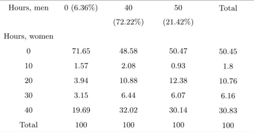
2[1−ρψˆ (Ziαˆ)]) (3.22) This represents the expected wage for non-worker i given the rth _{draw. Once} hourly gross wages are obtained for all the observations in the relevant sample, the tax-benefit simulator is used to get the net labour incomes for each possible choice of discrete worked hours. The discrete points are defined according to the observed distribution of worked hours. The graphs below show such a distributions for both men and women in couples21_.

21_{The graphs refer to the selected sample. The graph for men includes non participation. The graph for} women includes only the intensive margin (the participation rate for the selected sample of women is 49.7%).

(34)

According to these distributions, women in a couple are restricted to choose from the following discrete set: x={0, 10, 20, 30, 40}. These points correspond to the following intervals: 0-5, 6-15, 16-25, 26-36, >36. For married men we select the following discrete set: y={0, 40, 50}, which corresponds to the intervals: 0-10, 11-42 and >42. Since the labour supply for married female and men is estimated jointly, each couple has a choice set defined by the cartesian product y·x which leads to 15 possible combinations of discrete points.

The modified version ofMAPP02 computes total benefit entitlements and total tax amounts for each possible combination of discrete points given gross hourly wages. The algorithm takes time since for k possible choices of hours and 50

draws each non-worker hask50 diﬀerent net labour incomes. This means that the computational time increases exponentially when the choice set is expanded.

The net income for a particular alternative is computed by subtracting taxes and adding benefits plus non-taxable incomes to the gross labour income. This amount is then added up over the two spouses so as to get the total net household income.

Before proceeding with the estimation of the structural model, information on child-care costs and usage has to be collected from the ISTAT database. In this lat-ter database we first drop the households without children younger than 7 years be-cause for these households any information on child-care expenditures is recorded. Obviously, this represents a restriction due to data constraints but it must be pointed out that the school for kids is the most expensive one in Italy. Indeed, children that have turned six have access to the public school, which is basically free of charge.

Using only this sub-sample, we define 8 groups for child-care expenditure ac-cording to the presence of children aged less than 3, geographic area (northern, southern) and mother’s education (low or high). For each group we compute the distribution of hourly expenditure in formal child-care for those households ob-served demanding formal child-care. Then we approximate this distribution using 4 mass points. Next, we compute sub-groups controlling for the mother’s working status, which implies that 16 groups are now defined. For each of them we com-pute the percentage of households that have zero spending in child-care so that for each mother in each sub-group the probability of zero and positive spending is known.

(35)

like-3.5. Estimation procedure

lihood function. In practise, this means that for a mother in a particular group the likelihood is evaluated 5 times (when price=0, price=quartile1, p=quartile2, etc). Then, the expected contribution to the likelihood is computed using these probabilities as weights. The expected probability of choosing alternative j for observation i is then given by:

P r(pc = 0)P r(Hj|Xi,u, pc = 0) + 4 � s=1 [(1−P r(pc = 0))·0.25]P r(Hj|Xi,u, psc >0) (3.23) Where P r(Hj|Xi,u, psc) is the probability of choosing alternative j as defined

above.

The next step is to compute the statistical relationship between hours of work and hours of child-care. This is done by running simple OLS regressions for 6 groups defined by the number of children and their age, without controlling for any sample selection bias. Following Blundell et al. (2000) we assume a linear relationship between hours of work and hours of child-care so that for each group the following child-care cost function is estimated:

hcc=β0+β1hfj (3.24)

Whit this information it is possible to estimate the structural model. The estima-tion algorithm is implemented in Stata®_{. An overview of the Stata}® _{routine used}

(36)

3.6. Results from first-stage regressions

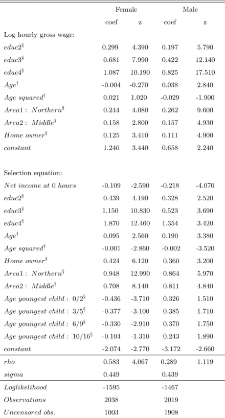
This section contains the set of estimates for the wage equations and child-care costs and usage. Table 1 presents the estimates of the wage equations for both female and male in couples. To identify the coefficients in the wage equations a set of instruments is used. This set includes dummies for the youngest child by age as well as the household income at zero hours of work for both the spouses. As it can be seen, all terms have the expected sign in both the selection equation and the main equation. In particular, the higher is the level of education achieved, the more likely is the participation in the labour market. The same is true if the couple does not live in southern Italy. All the coefficients in front of the instruments are significant for the female equation. In particular, female participation is lower when the couple has a child and this effect increases as the child’s age decreases. As expected, these variables are less or not significant for male but it is worth noting that they have the opposite sign with respect to female. Moreover, the higher are the non-labour sources of income the lower is the probability of participation for both the spouses. Finally, it is worth pointing out that the correlation coefficient between the two error terms - rho - is statistically different from zero and positive in both the equations.

(37)

3.6. Results from first-stage regressions

Table 3.1: Wage equations

Female Male

coef z coef z

Log hourly gross wage:

educ2§ 0.299 4.390 0.197 5.790 educ3§ 0.681 7.990 0.422 12.140 educ4§ 1.087 10.190 0.825 17.510 Age† _-0.004 _-0.270 _0.038 _2.840 Age squared† 0.021 1.020 -0.029 -1.900 Area1 : N orthern§ 0.244 4.080 0.262 9.600 Area2 : M iddle§ 0.158 2.800 0.157 4.930 Home owner§ 0.125 3.410 0.111 4.900 constant 1.246 3.440 0.658 2.240 Selection equation: N et income at0hours -0.109 -2.590 -0.218 -4.070 educ2§ 0.439 4.190 0.328 2.520 educ3§ 1.150 10.830 0.523 3.690 educ4§ 1.870 12.460 1.354 3.420 Age† _0.095 _2.560 _0.190 _3.380 Age squared† -0.001 -2.860 -0.002 -3.520 Home owner§ 0.424 6.120 0.360 3.200 Area1 : N orthern§ 0.948 12.990 0.864 5.970 Area2 : M iddle§ 0.708 8.140 0.811 4.840 Age youngest child: 0/2§ -0.436 -3.710 0.326 1.510 Age youngest child: 3/5§ -0.377 -3.100 0.385 1.710

Age youngest child: 6/9§ -0.330 -2.910 0.370 1.750 Age youngest child: 10/16§ -0.104 -1.310 0.243 1.890 constant -2.074 -2.770 -3.172 -2.660 rho 0.583 4.067 0.289 1.119 sigma 0.449 0.439 Loglikelihood -1595 -1467 Observations 2038 2019 U ncensored obs. 1003 1908

Note: Models estimated by Maximum Likelihood. † denotes that the variable is measured in terms of deviation from its mean. § denotes discrete variables. Educ$ are dummies that denote the achieved degree of education, the comparison group is the lowest level.

(38)

The next tables are related with the child-care demand. Table 2 reported below shows the distribution of child-care hourly expenditure for those households that are observed using child-care.

Table 3.2: distribution of hourly child-care cost (euro)

Groups: qtile: 12.5 qtile: 37.5 qtile: 62.5 qtile: 87.5 No kids<=3,South Italy,Low educ 0.180 0.276 0.468 1.920 No kids<=3,South Italy,High educ 0.223 0.325 0.446 1.560 No kids<=3,North of Italy,Low educ 0.333 0.499 0.669 1.404 No kids<=3,North of Italy,High educ 0.324 0.512 0.780 1.560 Kids<=3,South Italy,Low educ 0.195 0.312 0.390 1.560 Kids<=3,South Italy,High educ 0.217 0.364 0.702 2.184 Kids<=3,North of Italy,Low educ 0.429 0.758 1.443 3.432 Kids<=3,North of Italy,High educ 0.333 0.624 0.936 3.343 Note: sample size restricted to households with children in pre-school age.

As expected, the hourly child-care cost is higher, on average, in the northern Italy and among those households with children aged less than 3 years. Table 3 shows the proportion of each group and the probability of zero spending in child-care.

(39)

3.6. Results from first-stage regressions

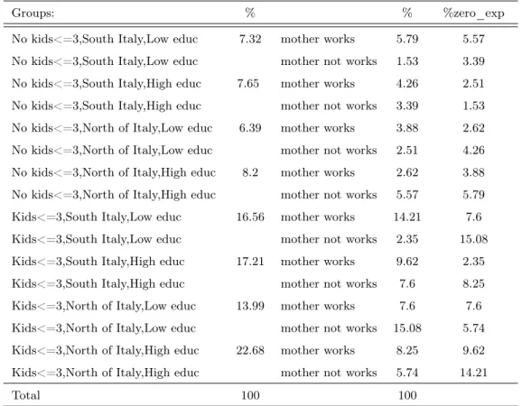
Table 3.3: Summary statistics for child-care usage

Groups: % % %zero_exp

No kids<=3,South Italy,Low educ 7.32 mother works 5.79 5.57 No kids<=3,South Italy,Low educ mother not works 1.53 3.39 No kids<=3,South Italy,High educ 7.65 mother works 4.26 2.51 No kids<=3,South Italy,High educ mother not works 3.39 1.53 No kids<=3,North of Italy,Low educ 6.39 mother works 3.88 2.62 No kids<=3,North of Italy,Low educ mother not works 2.51 4.26 No kids<=3,North of Italy,High educ 8.2 mother works 2.62 3.88 No kids<=3,North of Italy,High educ mother not works 5.57 5.79 Kids<=3,South Italy,Low educ 16.56 mother works 14.21 7.6 Kids<=3,South Italy,Low educ mother not works 2.35 15.08 Kids<=3,South Italy,High educ 17.21 mother works 9.62 2.35 Kids<=3,South Italy,High educ mother not works 7.6 8.25 Kids<=3,North of Italy,Low educ 13.99 mother works 7.6 7.6 Kids<=3,North of Italy,Low educ mother not works 15.08 5.74 Kids<=3,North of Italy,High educ 22.68 mother works 8.25 9.62 Kids<=3,North of Italy,High educ mother not works 5.74 14.21

Total 100 100

Note: sample size restricted to households with children in pre-school age. %zero_exp is the proportion of households that do not use formal childcare.

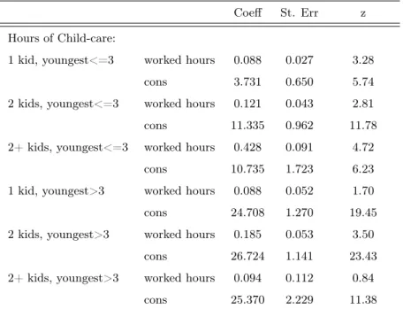
The proportion of households with zero spending provides evidence that house-holds with working mothers are more likely to buy formal childcare. Moreover, the probability of using child-care increases with the mother’s level of education and it is higher when the household lives in northern Italy. Finally, Table 4 shows the results of the OLS regressions for the relationship between hours of child-care and hours of work for the mother. The results are again presented by groups.

(40)

Table 3.4: OLS regression of child-care hours on worked hours

Coeﬀ St. Err z Hours of Child-care:

1 kid, youngest<=3 worked hours 0.088 0.027 3.28

cons 3.731 0.650 5.74

2 kids, youngest<=3 worked hours 0.121 0.043 2.81

cons 11.335 0.962 11.78

2+ kids, youngest<=3 worked hours 0.428 0.091 4.72

cons 10.735 1.723 6.23

1 kid, youngest>3 worked hours 0.088 0.052 1.70

cons 24.708 1.270 19.45

2 kids, youngest>3 worked hours 0.185 0.053 3.50

cons 26.724 1.141 23.43

2+ kids, youngest>3 worked hours 0.094 0.112 0.84

cons 25.370 2.229 11.38

Note: sample size restricted to households with children in pre-school age. OLS regression by groups.

As results provided show, the increment in child-care usage for a marginal incre-ment in the hours of work is higher when the couple has a child under three years old. This increment is higher when the household has more than two children and the youngest child is under three years old.

(41)

3.7. Results from structural model estimates

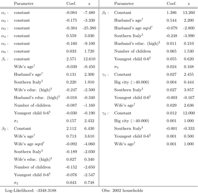
This section provides results for the structural model. The next table shows estimates for couples using 50 draws22_{. As it can be seen, most of the coeﬃcients}

have the expected sign. Importantly, fixed costs of working are both positive and highly significant at standard significant levels. On average, they turned out to be about €2000 per year. Since any restriction has been imposed a priori

on the coeﬃcient signs, it is important to verify the coherence of the estimated preferences with respect to standard textbook economic theory. In particular, it is crucial to check if the estimated utility function is quasi-concave in income for all the observations in the sample. I made this investigation by adapting the equations 3 and 4 in Van Soest (1995). As a result I found that the utility function is quasi-concave in income for 99% of the couples in the sample.

22_{The coeﬃcients obtained with 100 draws are not statistically significant from those obtained with 50} draws. This means that 50 draws are enough to ensure convergence.

(42)

Table 3.5: Structural model estimates for couples

Parameter Coef. z Parameter Coef. z

α1: constant -0.084 -7.480 β3: Constant 1.386 13.260

α2: constant -0.175 -3.330 Husband’s age† 0.544 2.200

α3: constant -0.384 -25.380 Husband’s age sqrd† -0.079 -2.800

α4: constant 0.559 3.030 Southern Italy§ -0.248 -3.990

α5: constant -0.160 -9.100 Husband’s educ. (high)§ 0.011 0.210

α6: constant 0.033 1.720 Number of children 0.065 1.530

β1: constant 2.571 12.610 Youngest child 0-6§ 0.055 0.620

Wife’s age† _-0.039 _-0.450 _σ

3 0.024 0.168

Husband’s age† _0.131 _2.300 _γ

1: Constant 0.027 2.455

Southern Italy§ _0.220 _1.910 _{Big city (>40.000)} _0.004 _0.444 Wife’s educ. (high)§ _-0.247 _-2.500 _{Southern Italy}§ _0.027 _3.857 Husband’s educ. (high)§ _-0.016 _-0.340 _{Youngest child 0-6}§ _-0.003 _-0.167 Number of children -0.087 -1.160 Wife’s age† _0.029 _2.636 Youngest child 0-6§ _-0.030 _-0.190 _γ

2: Constant 0.012 12.000

σ1 0.157 2.432 Big city (>40.000) 0.001 1.000

β2: Constant 2.112 6.430 Southern Italy§ -0.001 -0.333 Wife’s age† _0.713 _3.610 _{Youngest child 0-6}§ _0.001 _0.500 Wife’s age sqrd† _-0.092 _-4.060 _{Wife’s age}† _0.001 _1.000 Southern Italy§ _-0.189 _-2.030

Wife’s educ. (high)§ _0.027 _0.340 Number of children -0.152 -2.650 Youngest child 0-6§ _-0.076 _-2.547

σ2 0.043 0.748

Log-Likelihood: -3348.3188 Obs: 2002 households

Note: model estimated by Simulated Maximum Likelihood using Halton sequences (50 draws). Weekly household income divided by 1000; Women and men’s worked hours divided by 10; Random terms divided by 10;α2 andα3 divided by 100;α4divide by 1000. § denotes dummy variables and

†denotes that variables are measured in terms of deviation from their means. σs coeﬃcients are estimated standard deviations. The vectorsγ₁ andγ₂ represent fixed costs of working,γ₂ being the additional cost of working full time.

(43)

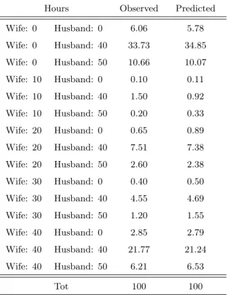
If we now turn on the estimated coefficients we can see that most of them are in line with standard economic guesses. Indeed, as expected, women preferences for work are decreasing with the number of dependent children, in particular when the youngest child is aged under than six. For men this pattern is exactly the opposite. Interestingly, preferences for work decrease for either spouses when they are from the southern of Italy and increase with own age at a decreasing rate. Women and men with high levels of education have increasing preferences for work. Finally, the standard deviation of the income coefficient is significantly different from zero indicating that unobserved heterogeneity in preferences for income exists in the sample. To check the ability of the model to fit the data, I computed average probabilities for each category of hours and compared with the observed frequencies. As it can be seen from the next table, the model is able to replicate observed frequencies quite well, in particular when women work more than 10 hours per week.

Table 3.6: Predicted vs observed frequencies

Hours Observed Predicted Wife: 0 Husband: 0 6.06 5.78 Wife: 0 Husband: 40 33.73 34.85 Wife: 0 Husband: 50 10.66 10.07 Wife: 10 Husband: 0 0.10 0.11 Wife: 10 Husband: 40 1.50 0.92 Wife: 10 Husband: 50 0.20 0.33 Wife: 20 Husband: 0 0.65 0.89 Wife: 20 Husband: 40 7.51 7.38 Wife: 20 Husband: 50 2.60 2.38 Wife: 30 Husband: 0 0.40 0.50 Wife: 30 Husband: 40 4.55 4.69 Wife: 30 Husband: 50 1.20 1.55 Wife: 40 Husband: 0 2.85 2.79 Wife: 40 Husband: 40 21.77 21.24 Wife: 40 Husband: 50 6.21 6.53 Tot 100 100

Once the parameters of the direct utility function are estimated, it is possible to compute the labour supply elasticities numerically following Creedy and Kalb

(44)

(2005). Firstly, gross hourly wages are increased by 1% and then a new vector of net household income for each alternative of hours is computed. Secondly, the probability of each alternative is computed for both the old and the new vector of net household income by means of the following probabilities:

P r(Hj|ypij,Xi) = 5 � s=1 P(ps_c|Xi) 1 R R � r=1 exp(U(yp_ij−T Cs ij,Hj,Xi,νr)) �K k=1exp(U(y p ik−T Ciks,Hk,Xi,νr)) (3.25) Withp=after, before. These probabilities are used to compute the expected labour supply for each spouse in the couple before and after the policy change23_:

E[Hs_|y_ip, Xi] = Js

�

j=1

P r(Hj|yijp,Xi)H_js (3.26)

Withs=men, women and p=after, before. Finally, the labour supply elasticity for each spouse in the couple can be computed numerically as:

εs= E[Hs_|_yaf ter i ,Xi]−E[Hs|yibef ore,Xi] E[Hs_|_ybef ore i ,Xi] · ₀_.1₀₁ (3.27)

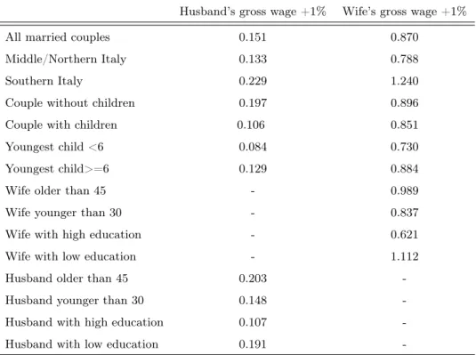
Withs=men, women. The next table shows such elasticities. However, it is worth noting that such elasticities have to be interpreted carefully. They are a useful summary measure of the labour supply behaviour but it has to bear in mind that they could vary substantially depending on the initial discrete hours level and the relative change in the gross hourly wages.

23_{Since husband’s earnings are on average bigger then the wife’s ones, I computed two sets of elasticities} derived from one percentage increase in either the woman gross wage and the man gross wage.

(45)

Table 3.7: Labour supply elasticities by individual characteristics

Husband’s gross wage +1% Wife’s gross wage +1%

All married couples 0.151 0.870

Middle/Northern Italy 0.133 0.788

Southern Italy 0.229 1.240

Couple without children 0.197 0.896

Couple with children 0.106 0.851

Youngest child <6 0.084 0.730

Youngest child>=6 0.129 0.884

Wife older than 45 - 0.989

Wife younger than 30 - 0.837

Wife with high education - 0.621

Wife with low education - 1.112

Husband older than 45 0.203

-Husband younger than 30 0.148

-Husband with high education 0.107

-Husband with low education 0.191

-Note: High education corresponds to secondary (5 years) or tertiary education.

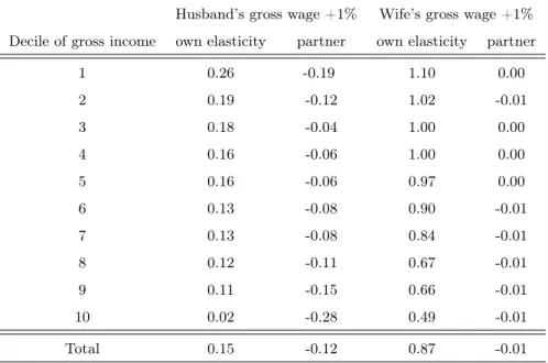
As it can be seen, labour supply elasticities by household characteristics are quite in line with the expectations. Female own elasticities are on average bigger than the male’s one. Moreover, elasticities are bigger in the southern Italy, for households without children and for partners without high education. The next table shows average elasticities for each decile of gross equivalent income24_{. As}

it was expected, elasticities are much more higher for low-income households and this is particularly true for the woman own elasticities. Finally, it can be noticed a intra-household substitution eﬀect between income and number of working hours of the partner.

24_{Equivalent gross household income corresponds to the gross household income divided by the square} root of the number of members.

(46)

Table 3.8: Average elasticities by 10 quantiles of equivalent income

Husband’s gross wage +1% Wife’s gross wage +1% Decile of gross income own elasticity partner own elasticity partner

1 0.26 -0.19 1.10 0.00 2 0.19 -0.12 1.02 -0.01 3 0.18 -0.04 1.00 0.00 4 0.16 -0.06 1.00 0.00 5 0.16 -0.06 0.97 0.00 6 0.13 -0.08 0.90 -0.01 7 0.13 -0.08 0.84 -0.01 8 0.12 -0.11 0.67 -0.01 9 0.11 -0.15 0.66 -0.01 10 0.02 -0.28 0.49 -0.01 Total 0.15 -0.12 0.87 -0.01

(47)

3.8. Concluding Remarks

This essay has explored the performance of the discrete approach for the estima-tion of labour supply elasticities for married couple using Italian data. The discrete approach has several advantages with respect to the continuous one. In particular, it easily allows for highly non-linear budget sets, non-participation, joint labour supply and endogenous child-care. Several innovations have been introduced with respect earlier Italian studies. In particular, we take into account unobserved het-erogeneity in preferences, child-care expenditures, errors in wage predictions and unobserved fixed costs of working. Estimated preferences are in line with the eco-nomic theory. In particular, the marginal utility of income is positive for 99% of the sample and preferences for work decrease with the number of young children and increase with age at a decreasing rate. Elasticities are derived numerically. As expected, the average elasticity of labour supply is higher for female in cou-ples, in particular for those who belong from low-income households. Average own elasticities are higher in southern Italy and they are lower for couples with young children.

(48)

3.9. Appendix

Overview of the STATA routine

Here we explain the routine we wrote for the optimisation algorithm. Stata® _has

a powerful built-in optimisation routine that is able to use, even within the same searching process, different optimisation algorithms such as Nr, Bhhh, Dfp, etc. There are three possible methods to maximise a self-written likelihood function. The first one, so-called method d0, requires the analyst to provide just the likeli-hood function. The second one, method d1, requires the computation of both the likelihood and the gradient. Finally, method d2, requires the computation of the likelihood, the gradient and the hessian. Whenever a piece of information is not provided, Stata computes it by numerical approximation, otherwise the algorithm just fill in the provided formula. Of course methods d2 and d1 are faster, more precise and stable but they are obviously time demanding. We chose method d0 for our program. The model to be estimated is the one described above. From a technical point of view it is a mixed conditional logit model. The difference with respect to a traditional conditional logit model is the presence of unobserved heterogeneity in preferences that has to be integrated out during the estimation process. This random terms are important because they relax the IIA assumption and give the model more reliability. Integrating out the unobserved factors (here also child-care prices and the unobserved part of wages for non-workers) produce a likelihood which is difficult to compute for the presence of a multidimensional integral. Instead of using traditional quadrature methods to approximate this inte-gral, we follow Train (2003) and use Simulated Maximum Likelihood with Halton sequences. The Stata® _command_mdraws _{by Cappellari and Jenkins (2003) helps}

to generate the Halton Sequences from which it is easy to get the correspondent draws from the multivariate normal distribution. we call the constructed draws

random1_r, random2_r, etc. Notice that r denotes the draw and 1,2,... identify the random terms. Formally, the utility we defined in the Stata® _{routine is:}

U(yij;Hj;Xi) = α1y2ij+α2hfj2+α3hm2j+ +α4hfjhmj +α5yijhfj +α6yijhmj+ +(β₁x�₁+ν1)yij + (β2x � 2+ν2)hfj + (β3x � 3+ν3)hmj (3.28) Where: