Effect of lip shape on shock wave-boundary layer interactions in transonic intakes at incidence

Effect of Lip Shape on Shock Wave-Boundary Layer

Interactions in Transonic Intakes at Incidence

A. Coschignano∗_{and H. Babinsky}†

Department of Engineering, University of Cambridge, Cambridge, CB2 1PZ, UK C.Sheaf‡and G.Zamboni§

Installation Aerodynamics, Rolls Royce Plc., Derby, DE24 8BJ, UK

The flow field around five transonic inlet lips at high incidence is investigated for a variety of flow conditions around a design point representative of a take-off scenario. Generally, the flow on the surface of the lip is characterised by a supersonic region, terminated by a near-normal shock wave. For the baseline lip profile at the nominal design point, the shock is not strong enough to cause large flow separation, resulting in marginal losses in pressure recovery. Four more parametric shapes were investigated at this design point, obtained by changing the aspect ratio and ‘sharpness’ of the super ellipse defining the lip contour. Furthermore, off-design conditions are also explored by altering the angle of incidence as well as changing the mass flow rate over the lip, intended to mimic the effect of an increase in engine flow.

The parametric investigation revealed a significant effect of lip shape on the position and severity of the shock wave-boundary layer interaction. In particular, the high aspect ratioslim

nacelle performed poorly, favouring shock development very close to the lip nose and promoting large scale separation as the incidence increases.

From correlation studies based on the parametric investigation, it appears that the extent of shock-induced separation is the main factor affecting the aerodynamic performance. Somewhat surprisingly, this was found to be independent of shock strength but potentially related to the severity of the diffusion downstream of the shock. Alongside delaying flow reattachment, this diffusion is also likely to have a direct detrimental effect on the boundary layer development close to the engine fan.

Nomenclature

α Angle of incidence

δ Boundary layer thickness

δ∗ _{Boundary layer displacement thickness}

θ Boundary layer momentum thickness

c Intake chord length H Shape factor

L∗ Interaction length Û

m Mass flow

m(x) Super ellipsexexponent

n Super ellipseyexponent M Mach number

P Pressure

Re Reynolds number (based on lip thickness)

Rc Inlet highlight radius of curvature

s Stream-wise distance along surface tm Intake maximum thickness

U Flow velocity

∗_{PhD Candidate, Department of Engineering, University of Cambridge, AIAA Student Member.}

†_{Professor of Aerodynamics, Department of Engineering, University of Cambridge, AIAA Associate Fellow.} ‡_{Installation Aerodynamics, Rolls Royce Plc.}

x Stream-wise direction, parallel to lab floor

y Vertical direction, normal to surface model, unless otherwise stated

z Span-wise direction. AR Intake aspect ratio

LDV Laser Doppler velocimetry PSP Pressure sensitive paint

SBLI Shock-wave boundary layer interaction

V E PVirtual Engine Plane, x=2.4tm,baseline

Subscript

0 Stagnation value

1 Property upstream of the shock

e Free-stream property

l Lower channel, usually referred to mass flows

i Incompressible property

u Upper channel, usually referred to mass flows

I. Shock-Boundary Layer Interactions in Subsonic Engine Intakes

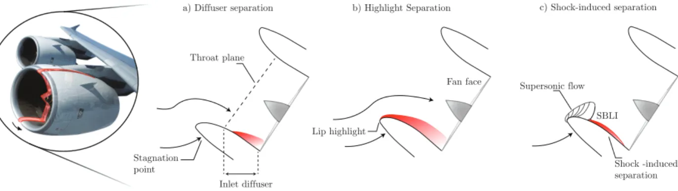
During off-design operations such as high-incidence scenarios the inlet aerodynamic performance is dominated by the flow distortion around the lower lip. The flow stagnates on the outer surface of the nacelle and, as incidence or mass flow rate increase separation potentially occurs in the diffuser or at the highlight (inlet leading edge), with the latter indicating a fully stalled intake [1]. A schematic depiction of the two separation types is presented in Figure 1a-b. Furthermore, a number of sources [1, 2] observed a sharp loss in pressure recovery for high mass flow rates (i.e.: yielding an average Mach number at the throat plane in excess of Mt ≥0.7). This was attributed to the formation of normal shock-waves within the inlet causing shock-induced separation of the boundary layer, as schematically depicted in Figure 1c.

In recent years, in order to reduce emission and increase efficiency, engine manufactures are pursuing larger, more efficient engines. As the engine size increases, a slimmer nacelle is generally preferred to reduce form drag during cruise and to avoid ground clearance problems. However, this design choice could promote large scale separation during off-design operations such as high-incidence scenarios and manoeuvring at the edge of the design envelope. Furthermore, the effect of lip geometry on the development of shock wave-boundary layer interaction inside the nacelle is still not well understood: whereas the design ofshock-freeaerofoils has been extensively pursued in order to delay detrimental effects such as drag rise and buffet onset, a design philosophy aimed specifically towards tackling the problem of shock formation in intakes has yet to arise.

Fan face

Inlet diffuser Stagnation

point

Lip highlight

a) Diffuser separation b) Highlight Separation

Supersonic flow SBLI Shock -induced separation c) Shock-induced separation Throat plane

Fig. 1 Schematics of an inlet cross section during high incidence flight: a) Flow separating in an intake diffuser; b) separation occurring at the lip highlight (intake stall). c) Shock induced separation over the lower lip.

Earlier analytical studies [3] and experiments [1, 2, 4] showed a significant effect of lip geometry and inlet contraction on the Mach number distribution over the lower lip during hig incidence conditions. However, due to the inability

of analytical models to account for complex phenomena such as SBLI and the poor resolution of the experiments, shock-wave boundary layer interactions were not taken into account.

However, in a real intake flow, the interaction of incoming boundary layers with shock waves of different strength can have drastically different outcomes, with tangible impacts on the flow stability downstream. It would appear that the available literature is rather scarce and, due to the limitations of experimental set-ups and analytical models, unable to assess the nature and severity of shock wave boundary layer interactions.

In sight of the up-coming inlet reshaping, understanding the onset of detrimental effects associated with high incidence flight might contribute to future designs that would allow engine inlets to operate more efficiently over a wider range of conditions, including limit manoeuvring and off-design scenarios involving SBLIs.

This paper aims to identify the main factor affecting the boundary layer development downstream of a normal shock wave -boundary layer interaction. Four inlet lip variations are considered here, along with a representative inlet shape (based on a current inlet geometry and amply discussed in a previous paper [5]).

A. Target flow-field and working section design

The problem is simplified by noting that high incidence operation reduces the area of aerodynamic interest to the lower lip only. It is assumed that the length-scale of tangential changes along the nacelle circumference is of the order of its curvature radius. This is noticeably larger than the lip radius and thickness, which could be considered representative length-scales of the stream-wise and normal changes along the lip. Thus, only a cross section along the centre span of the intake is considered and the lower lip is treated like an aerofoil. As a result, a nominally 2D experimental set-up is used here.

To delimit the experimental domain, a stream-tube geometry in the symmetry plane was extracted from 3D RANS computations of a typical engine flow and used to define the wind tunnel working section depicted in Figure 2. Subsequently, the set-up was fine tuned, as described in detail in §I.C, in order to obtain a pressure distribution matching experimental tests on a 3D nacelle deemed representative of high-incidence manoeuvring and defining the current experiment baseline.

The baseline lip geometry used here is a generic lip shape (defined in §I.E) designed to generate a pressure distribution, shock strength and location comparable to the aforementioned 3D tests.

B. CUED blow down wind-tunnel

Variable area 2nd _throat Working Section Streamtube Settling Chamber Seeding rake 18:1 contraction Pressure port Turbulence screens Honeycomb straighteners High pressure reservoir S Seeder supply Measurement probe α

Adjustable plug to chocke section Fig. 2 Representation of the blow-down wind tunnel facility. Flow from left to right. Stream-tube design based on computed flow streamlines selected by Makuni [6].

The blow-down wind-tunnel assembly is schematically depicted in Figure 2. The wind-tunnel is powered by two 50 kW compressors. The flow is fed from the compressors into the settling chamber, where it is passed through a number of flow straighteners and turbulence grids before a 18:1 contraction. The entry Mach number is varied by adjusting the effective area of the second throat where the flow is chocked by means of an aerofoil (see RHS of Figure 2). Changing the total pressure allows some degree of variation in Reynolds number.

ratio between the mass flow rates in each channel provides an effective way to control a third variable: the engine mass flow demand. In a real intake, when engine mass flow rate varies, so does the stagnation streamline dividing the flow going into the intake from that spilled along the outer nacelle. During high incidence operation, this streamline comes to rest on the outer surface of the lip. As the amount of air captured by the intake increases, the stagnation streamline shifts further down onto the lower surface. In the experimental facility, this is replicated by using a choking rod in the lower channel as highlighted in Figure 2. The latter allows a fine control (∆mÛl <0.1%mÛ) of the mass flow discharged via the lower passage. To investigate the response to stagnation streamline changes, the overall mass flow is kept constant at the reference value while the mass flow rate through the lower passage is progressively reduced. This forces a greater proportion of the mass flow inside the upper channel, effectively mimicking a greater demand by a turbofan engine. An increase inmÛuby 15±0.3% over the reference value has been considered here. The model incidence is varied between 23◦and 25◦.

C. Matching the target flow-field - Reference operating conditions

This section presents the operating parameters of the current facility that result in a flow-field closely matching a typical high-incidence condition for the baseline geometry.

A Reynolds number (based on maximum thickness and inflow velocity)Ret ≈1.10×106, representative of a full scale, small sized engine at sea level, is used to achieve a good compromise between dynamic similarity and run time. This value is obtained with a stagnation pressure of 211kPa. To match the 3D tests pressure distribution, the model incidence was set at 23◦_{and the entry Mach number set to M}

∞=0.435±0.0005. The choking rod is set so that∼74%

of the total mass flow is discharged via the upper channel. The operating conditions are summarised in Table 1. A number of off-design conditions are also explored. However, for practical reasons the geometry of the stream-tube defining the working section, based on stream-lines of the baseline flow-field extracted from a RANS CFD solution, was kept constant throughout the whole investigation. It can be argued that every operating point requires a new stream-tube geometry as the flow streamlines may change. Although an effect of the stream-tube geometry might be expected, this should not affect the main conclusions for a number of reasons: near the area of interest, the streamlines do not show a very pronounced curvature; moreover, at the design stage the upper bound of the working section was chosen to be sufficiently far from the supersonic region [6].

Furthermore, the changes in operating conditions around the design point are relatively minor: the highest increase in incidence from the baseline value is of only 2◦. Moreover, the maximum increase in upper channel mass flow rate is limited to 15% of the initial value. Finally, the changes in the flow-field across the shapes tested is not so drastically different to suggest a reshaping of the wall to be necessary.

Table 1 Inflow conditions for the reference scenario. These are kept constant for each geometry tested. Û

m(kg/s) Mentr y α(deg.) P0(kPa) T0(K)

Û

mu

Û

m Ret

8.68 0.435 23 211.6 290±4 ∼3.8 ∼106

D. Experimental methods and errors

A Schlieren technique is used to visualize the features typical of compressible flow-fields. A horizontal knife edge is used and the images were captured at a rate of 4000fps at a resolution of 1024×512 pixels.

Surface pressure measurements in the centre-span are taken using tappings connected via tubing to a differential pressure transducer. Though small in diameter, the presence of a cavity can result in an over-prediction of static pressure by approximately 0.5%-1.0% according to Meier [7].

A number of these pressure readings are used to calibrate pressure sensitive paint (PSP). According to Gregoryet al. [8], 5-6 different known pressure values are usually sufficient to minimise error. In the current investigation, the mean deviation between the values extracted form the paint and that measured using the surface taps is found to be ranging from approximately 2% to a maximum of 4%.

Flow velocities in the tunnel centre-span are measured using a two component Laser Doppler Velocimetry (LDV) system. The ellipsoidal working volume measures 130µm in diameter. Paraffin particles, with a diameter of approximately 0.5µm [9], are used to seed the flow. The laser emitting head and receiving optics are mounted on a three-axis traverse. The signal is sampled at an optimised variable rate to exploit a full signal cycle leading to a typical measurement accuracy, as stated by the manufacturer, of±0.1% ofUmax(∼580m/s) [10]. In addition the emitting head

is oriented at an angleβ= 8.5◦from the horizontal. A component of the span-wise velocity,w, therefore affects the measurement of vertical velocity component. On the symmetry plane, where measurement are taken,wis expected to be one order of magnitude lower thanv. As a consequence of this and of the small angle, the error invis expected to be just above 1%. The stream-wise velocity componentuis unaffected byβ.

The other source of uncertainty is related to velocity bias. According to the findings of both McLaughlinet al. [11] and Buchhaveet al. [12], the error is expected to be between 5% and 10% ofU0. For the current investigation the error due to velocity bias is not expected to exceed 4% near the wall. The vast majority of measurements are expected to have an average uncertainty around 1.5%.

Velocity measurements are used to estimate the incompressible boundary layer integral properties, which relies on integration of the velocity profile from the wall to the boundary layer edge. However, the measurement probe is of finite size and measuring any closer than 0.2mm from the wall is infeasible. Furthermore, numerically integrating over discrete data points can yield significant error. To address these shortcomings, an analytical boundary layer profile is fitted to the data points before integration.

The model by Sun & Childs [13], which builds on the classical linear combination of the law of the wall and Coles’ wake function [14], has been used in the Cambridge facility for several years. Sun & Childs’s models is valid down toy+≈100. For the buffer and viscous layers, the relationship proposed by Musker is used [15] to obtain complete solution for 0≤y≤δ. The integral parameters can be calculated by simple numerical integration. A comprehensive investigation of the validity of this method has been performed by Titcheneret al. [16]. The main sources of errors were found to be the resolution of discrete data points and misalignment of the wall position. In particular, the number of points necessary for the error to be≤5% is inversely proportional to the boundary layer shape factor but approximately 20-30 points inside the boundary layer are sufficient to achieve an error under 5% for a range of shape factors. This condition is generally satisfied in this investigation. Overall, the error is expected to be<2% for the largest kinematic shape factor and<5% for the thinnest, healthiest, boundary layers.

Wall offset was found to cause a significant error in integral parameters [16]. A small misalignment of∆y/δof the order of 0.01 yields an error exceeding 5%. For the worst case scenario, defined by a thicknessδ=1.98 mm, the wall location is accurate within∆y/δ≤0.005. This places the outer error boundary to ≤2%.

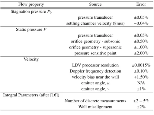
A summary of experimental error is given in Table 2.

Table 2 Summary of experimental errors

Flow property Source Error

Stagnation pressureP0

pressure transducer ±0.05% settling chamber velocity (8m/s) −0.04% Static pressureP

pressure transducer ±0.05% orifice geometry - subsonic ±0.50% orifice geometry - supersonic ±1.00% pressure sensitive paint ±2.00% Velocity

LDV processor resolution ±0.0015% Doppler frequency detection ±0.10%

velocity bias near the wall +1.50%

emitter angle,u N/A

emitter angle,v ±1%

Integral Parameters (after [16])

Number of discrete measurements ±2−5%

E. Intake Lip Design

The inlet lip shapes have been designed by using a modified super ellipse profile. Mathematically, a modified super ellipse is defined as:

_x−_a a m +y b n =1 (1) with m(x)=2+ x a 2 (2) whereaandbare the major and minor axis of the ellipse, respectively controlling the position and the size of the ellipse co-vertex. In intake terms, this point indicates where the intake is at its thickest, i.e.: the throat. Figure 3 depicts the coordinate system (originating at the lip highlight) and illustrates how the parameters defined in Equation 1 relate to the design of the intake lip model. The ratioa/bis defined as the aspect ratioARof the ellipse. Its powers, on the other hand, set the locus of the point of maximum curvature.

RTh RHl a b Fan face Center-Line Modified super ellipse Diffuser Throat Highlight x s y

Model trailing edge

tm

Fig. 3 Cross section of the model depicting the intake geometry definition, modified super ellipse in red. Coordinate s is defined as arc length along the lip.

This type of ellipse results in a continuous reduction in curvature from the highlight to the throat. Downstream of this, the geometry was tailored to replicate a typical diffuser shape. This is virtually identical for the lip profiles define by a varying highlight sharpness but varies slightly across different aspect ratio lips to ensure a uniform curvature distribution.

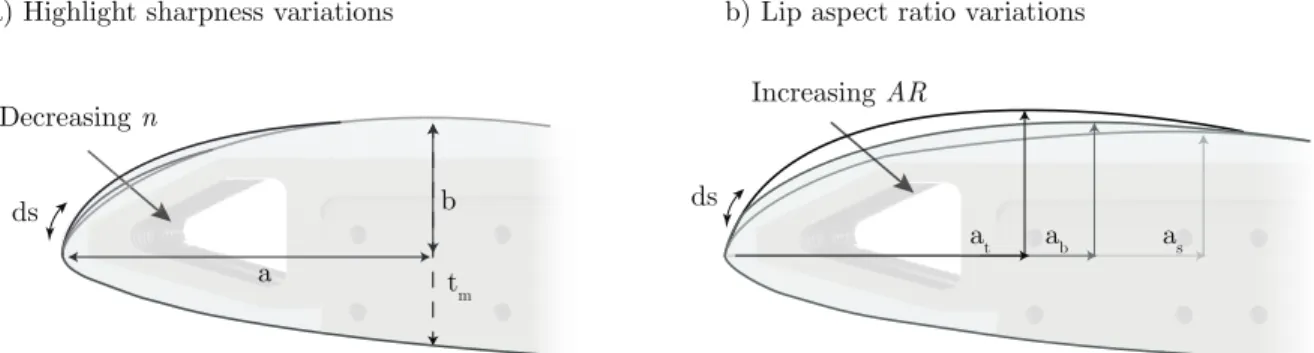
The baseline lip is defined by an aspect ratioAR=2.75 and a value ofn=2. Four other lip geometries have been investigated. These include two highlight and two aspect ratio variations over the baseline, as depicted in Figure 3. The geometry definition for each shape is given in Table 3. The external fore-body geometry is based on a generic intake and is the same for every geometry tested herein.

Table 3 Geometry definition for constant aspect ratio lips Profile n AR Rc|LE(mm) Baseline 2 2.75 5.5 Sharp 1.7 2.75 3.1 Blunt 2.2 2.75 7.0 Slim 2 3.63 4.3 Thick 2 2.10 9.3

Increasing AR ds a_t a_b a_s Decreasing n a ds b t_m

a) Highlight sharpness variations b) Lip aspect ratio variations

Fig. 4 a) Lip highlight geometries obtained by changing the super ellipse exponentnb) Lip geometries obtained by changing the super ellipse aspect ratio. Geometry definition provided in Table 3.

II. Results

Time averaged (across 0.5s) Schlieren photographs of the highlight region for the five shapes and two incidence levels of 23◦_{and 25}◦_{are shown in Figure 5 and Figure 6 respectively, providing a first qualitative outlook of the flow}

field. At the lower incidence, around the baseline lip highlight, the flow undergoes rapid acceleration. A very dark region in the immediate proximity of the highlight can be seen in the Schlieren image. This is likely to be caused by the very strong density gradients around the lip highlight. The bright area in Figure 5b is caused by the strong expansion in the supersonic region. This is terminated downstream by a normal shock, which appears in the Schlieren photograph as a dark line approximately normal to the surface. Downstream of the shock, the boundary layer is clearly visible and can be seen to grow along the surface.

At the reference incidence at least three shock waves can be observed over thesharplip. In proximity of the highlight, expanded in Figure 5a, a dark line is seen followed by a bright one. This indicates a compression (potentially through a first weak shock-wave) and subsequent re-expansion, which is terminated by a shock downstream. A subsequent bright area follows, signifying a further expansion stage. The last terminal shock wave appears very weak and located further downstream compared to both other cases. For both shock waves, noλfoot is observed.

The flow field around the blunter profile in Figure 5c does not appear significantly different from the baseline. The shock position is similar, although a marginally more smeared interaction region can be seen.

A strong effect of aspect ratio on shock position is noted. For the highest aspect ratioslimlip, the shock wave is noticeably upstream compared to the baseline, very close to the highlight. On the other hand, the shock sits closer to the throat plane for the lowest aspect ratiothicklip. The averaged images for this shape show a modest smearing of the shock, indicating potentially larger shock motion.

At 25◦, a single shock is present over every lip considered. Generally, observing the time averaged images, a greater smearing of the interaction is seen at 25◦compared to 23◦, suggesting a more pronounced shock motion as incidence is increased further. Compared to the baseline, the terminal shock for thesharplip is further downstream. On the other hand, the shock over thebluntprofile sits upstream compared to both the baseline and same shape at lower incidence. From Schlieren, thebluntlip appears to displays a degree of shock oscillation comparable to the baseline.

The flow over theslimlip at 25◦appears to separate very close to the highlight, where a thickening of the boundary layer is observed from averaged pictures. The onset of this thickening corresponds roughly with the front leg of aλ shock. Further downstream, a number of secondary shocklets can be observed.

From Figure 6c (bottom), the position of the shock over the thicker nose appears similar to the reference incidence of 23◦. A more smeared shock is however seen.

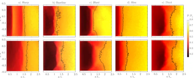
Wall pressure measurements are shown in Figures 7-8 for incidence levels of 23◦(top) and 25◦(bottom) respectively. The pressure along the centre-span of the model is given in Figure 9.

At 23◦_{, due to poor optical access near the highlight, the first SBLI over thesharplip could not be resolved. The two}

subsequent shocks show an exceptional two dimensionality. The baseline andbluntlip show a broadly similar pressure field, characterised by a single pressure rise and modest corner effects.

Over the slimmer lip, the extent of the supersonic region is considerably smaller than the baseline, with a terminal shock located at s≈0.5tm. This shape also shows the greatest degree of two-dimensionality. This is generally found

a) Sharp b) Baseline c) Blunt d) Slim e) Thick Reference ṁ u +15%ṁ u 1 2 3

Fig. 5 Time averaged (∼0.5 s) Schlieren images for the five shapes at 23◦and two mass flow rates.

a) Sharp b) Baseline c) Blunt d) Slim e) Thick

+15 u % ṁ u Reference ṁ u

Fig. 6 Time averaged (∼0.5 s) Schlieren images for the five shapes at 25◦and two mass flow rates.

in the presence of a weak centre-span interaction resulting in small or absent separation. From Figure 9, using the smearing of the pressure rise between the onset and the isentropic sonic line as an indication for the size of separation [5], it seems likely that a recirculating region is present for each lip; this is expected to be larger for thethicklip.

As the incidence is increased to 25◦, for the baseline case the onset of pressure rise in the centre-span is found at a stream-wise position along the surface ss≈0.9tm. This is similar to the baseline incidence. The estimated mean separation size, which was found [5] to be correlated to the distance between the shock and the isentropic sonic line in Figure 9, is expected to have grown in size as there is an increasingly greater smearing of the pressure rise. Furthermore, a more extensive region of smeared pressure near the corners is observed at higher incidence.

At 25◦the SBLI over thebluntlip exhibits an upstream shift of the shock compared to the reference incidence, as previously observed in the Schlieren images in Figure 6. The distance between the sonic line and thebluntlip centre-line pressure rise onset is greater than the reference incidence, implying extensive separation.

Wall pressure measurements at 25◦, reflect the largely separated flow near the highlight of theslimlip. For thethick lip, the onset of pressure rise is found marginally upstream compared to the reference incidence. The pressure smearing is comparable to the baseline.

From Figure 9, it appears that lip shape has a strong effect on both the peak isentropic Mach number (low pressure) and position of the pressure rise. Although some degree of subjectivity is involved when defining a ‘good intake’, a thin boundary layer with a low momentum deficit θi at the nominal engine fan location, can be considered a positive performance indicator. In order to assess the effect of the imposed pressure distribution on the boundary layer downstream of the interaction, velocity measurements are taken near the plane where an engine face would sit. As shown in Figure 10, the measurement plane, referred to as theVirtual Engine Plane(VEP), is at x=2.4tm. Measurements are shown for both families of parametric shapes and incidence levels in Figure 10. The boundary layer integral properties obtained from the data in Figure 10 are summarised in Table 4 and Table 5 for the baseline and the four variations respectively.

At the reference incidence of 23◦, the boundary layers for the two aspect ratio variations are of similar size at the VEPand almost twice as thick compared to the baseline case. Looking at each lip specifically, the integral parameters for thethicklip in Table 5 reveal the greatest displacement and momentum thicknesses, roughly twice the baseline values.

Fig. 7 Wall pressure estimated using PSP for the five shapes considered at 23◦for the referencemÛu(top) and +15% increment (bottom).

Fig. 8 Wall pressure estimated using PSP for the five shapes considered at 25◦for the referencemÛu(top) and +15% increment (bottom).

Theslimlip values are somewhere in the middle,∼50% greater than the baseline. However, it is noted that the highest aspect ratio lip has the lowest measured shape factor of Hi =1.277, indicative of a very healthy boundary layer. At the reference incidence, thebluntlip values ofδare almost double that of the baseline andsharplip counterparts, which are of comparable size. Despite the larger size, momentum and displacement thicknesses are only marginally greater than the values for the baseline andsharplip boundary layers, which are considerably thinner. In addition, the bluntlip displays the fullest velocity profile.

On the other hand, shape factor for thesharplip is the highest measured at Hi=1.52. The high shape factor could be caused by the multiple shock-adverse pressure gradients hindering the full recovery of the boundary layer. Another explanation could be advanced if, as suggested by the low Mach number and pressure measurements, an attached interaction is assumed, which results in a generally more gradual boundary layer recovery compared to separated SBLIs [17] and, in adverse pressure gradients, recovery can be expected to be delayed even further.

At higher incidence the differences in boundary layer properties at the VEPfor the different shapes are more pronounced. The slimmer lip integral parameters reflect the consequences of the largely distorted flow field seen in Schlieren images (Fig. 5-6) and PSP (Fig. 8). The boundary layer is the thickest measured across any shape, almost twice the baseline value at 25◦. The displacement and momentum thicknesses are also the highest at approximately 2.5

0.5 1 1.5 2 2.5 0.2 0.3 0.4 0.5 0.6 0.7 0.5 1 1.5 2 2.5 P/ P0 s/tm s/tm Sharp Blunt Slim Thick Baseline 0.5 1 1.5 2 2.5 s/tm 23° 25° 23°, +15% ṁ 25°, +15% ṁ 0.5 1 1.5 2 2.5 s/tm

Fig. 9 Centre-span pressure (solid line: PSP; symbols: transducer values) for each lip at two incidence levels and upper channel mass flow rate values.

times the baseline values at the same incidence. The shape factor exceeds 1.8 and is also the highest measured value at 25◦.

Thethicklip shows more modest increases in integral properties compared to the reference incidence, in line with other shapes and the baseline case.

From Figure 10 and Table 5, it can be seen that thesharplip behaves differently than other cases at higher incidence. While both other geometries display a considerable BLthickening accompanied by a deterioration of all integral properties as the incidence increases, thesharplip shows no significant change inδ. Furthermore, both displacement and momentum thicknesses are seen to decrease at higher incidence. The measured shape factor at 25◦is lower than at 23◦and than any other geometry at 25◦.

0.5 0.6 0.7 0.8 0.9 1 U/Ue U/Ue 0 0.2 0.4 0.6 0.8 1 y/δ 0 0.2 0.4 0.6 0.8 1 b) 23° c) 25°

a) Location of wall normal measurements

0 0.5 1 1.5 2 2.5 3 3.5 4 x/tm

2.4tm _VEP y

Fig. 10 a) Location of the reference plane (VEP) near the nominalengineface. b) Wall normal measurements at the reference plane at 23◦. c) Wall normal measurements at 25◦. An analytical model is fitted to the data to obtain a continuous velocity profile. _NSharp;Baseline;_IBlunt;_HSlim;Thick. Open symbols: +15%mÛu

III. Factors influencing intake performance

The purpose of an intake is, by definition, to provide good quality flow at the engine face or, in other words, a thin and full boundary layer across the operating envelope. Ultimately, the boundary layer development depends primarily on the imposed pressure distribution. Along the lips investigated here, several regions of characteristic pressure gradients are identified: strongly favourable around the nose; a narrow re-compression region ahead of the shock; the shock pressure jump; the rise in pressure in the diffuser between the shock and theVEP. In order to determine whether any of these regions has a more dominant role, this section explores correlations between different parameters, concentrating on those deemed most likely to affect the boundary layer development: the strong adverse pressure gradient regions.

Table 4 Incompressible boundary layer parameters for the baseline lip at theVEP. α(◦) mÛu δ/tm δ∗_i/tm θi/tm Hi 23 Ref. 0.074 0.010 0.0078 1.345 +15% 0.087 0.010 0.008 1.297 25 Ref. 0.158 0.030 0.0210 1.465 +15% 0.175 0.035 0.0236 1.488

Table 5 Incompressible boundary layer parameters for the four lip geometries considered at theVEP.

(a)Sharp α(◦_{) mÛ} u δ/tm δ∗_i/tm θi/tm Hi 23 Ref. 0.064 0.013 0.0087 1.526 +15% 0.057 0.010 0.007 1.436 25 Ref. 0.066 0.011 0.0081 1.424 +15% 0.072 0.014 0.009 1.481 (b)Blunt α(◦_{) mÛ} u δ/tm δ_i∗/tm θi/tm Hi 23 Ref. 0.127 0.0158 0.0122 1.301 +15% 0.166 0.022 0.016 1.301 25 Ref. 0.250 0.056 0.0358 1.556 +15% 0.240 0.053 0.0342 1.552 (c)Slim α(◦_{) mÛ} u δ/tm δi∗/tm θi/tm Hi 23 Ref. 0.137 0.0155 0.0121 1.277 +15% 0.170 0.0172 0.0134 1.282 25 Ref. 0.297 0.087 0.0473 1.833 +15% 0.288 0.088 0.0462 1.900 (d)Thick α(◦_{) mÛ} u δ/tm δi∗/tm θi/tm Hi 23 Ref. 0.1435 0.023 0.0166 1.378 +15% 0.173 0.0289 0.0207 1.394 25 Ref. 0.2029 0.048 0.0298 1.601 +15% 0.223 0.0499 0.0319 1.562

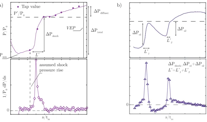
Figure 11a illustrates the different regions for a typical centre-span pressure rise. The total pressure rise is the delta between the minimum pressure (peak isentropic Mach number) and the value at theVEP. The shock∆P, indicative of its strength, is the difference between the isentropic sonic line, where P/P0 =0.528, and the value at the pressure rise onset. The latter is taken at the point where the pressure gradients show an upward kink. The pressure rise in the diffuser is the subsequent increase between the sonic value and the pressure measured at theVEP. The interaction length is taken as the stream-wise distance between the pressure rise onset and the isentropic sonic line. BothmÛu values and incidence conditions are used for the correlations.

A special definition is required by thesharplip at 23◦incidence and referencemÛu. The pressure and pressure gradient distributions are shown in Figure 11b. In §II.A, this lip was found to result in a multiple shock system. The small shock in the immediate proximity of the highlight could not be resolved due to poor optical access and only the two downstream shocks are taken into account. As shown in Figure 11b, the interaction length is taken as the sum of the two individual interaction lengths∗. The shock pressure jump is also taken as the sum of the individual pressure rises across the two shocks. In addition to the unique pressure distribution, the low shock Mach numbers measured for this configuration could imply the absence of shock-induced separation, while all other interactions are expected to be separated. As a result,sharplip results at 23◦incidence are plotted here as a grey triangle and should be treated with care.

The main indicator of aerodynamic performance is chosen to be the momentum thicknessθiat theVEP, being a measure of lost momentum. Shape factor Hi and boundary layer thicknessδare also considered.

∗_{since the pressure does not reach the sonic value,L}∗_{for the first shock has been defined as the distance between the pressure rise onset and the}

Figure 12 shows the variation ofδ, θi and Hiwith total pressure rise. Each shape is assigned a different symbol as indicated in the caption. Considerable scattering is present but larger values ofδ,θi and Hi appear to be mostly associated with a higher total pressure rise. The largely separatedslimlip at 25◦lies off this trend.

The variation of the boundary layer parameters with∆Pshock is presented in Figure 13. For every boundary layer parameter considered, the amount of scattering would suggest that there is no meaningful correlation with the shock pressure jump, which is somewhat surprising. In fact, a number of shapes characterised by the same shock pressure jump have drastically different values forδ, θiand Hiat theVEP.

P/P 0 1/P 0 dP/ds s/t_m Tap value P*_/P 0 assumed shock pressure rise L* ΔPshock ΔPdiffuser VEP _ΔP total P_min s/t_m 0 0

a)

b)

Fig. 11 a) Definition of the pressure rise stages along the lower lip and of the interaction lengthL∗. b) Shock pressure rise andL∗definitions for the peculiar sharp lip at 23◦.

0.3 0.36 0.42 0.48 δ/t m Hi θi /tm 1.2 1.4 1.6 1.8 2 0.05 0.1 0.15 0.2 0.25 0.3 0.35 0.01 0.02 0.03 0.04 0.05 ΔPtotal/P0 0.3 0.36 0.42 0.48 ΔPtotal/P0 0.3 0.36 0.42 0.48 ΔPtotal/P0

Fig. 12 Variation of selected boundary layer properties at the VEPwith total pressure jump. _NSharp; Baseline;_IBlunt;_HSlim;Thick. Open symbols: 25◦_.

Figure 14, on the other hand, shows the correlation between the boundary layer parameters and the pressure rise in the diffuser. Large scattering is present but it can be noted that higher values ofθi are found with a greater diffuser

0.1 0.15 0.2 0.25 0.3 0.35 0.1 0.15 0.2 0.25 0.3 0.35 0.1 0.15 0.2 0.25 0.3 0.35 ΔPshock/P0 δ/t m Hi θi /tm 1.2 1.4 1.6 1.8 2 0.05 0.1 0.15 0.2 0.25 0.3 0.35 0.01 0.02 0.03 0.04 0.05 ΔPshock/P0 ΔPshock/P0

Fig. 13 Variation of selected boundary layer properties at theVEPwith shock pressure jump. _NSharp; Baseline;_IBlunt;_HSlim;Thick. Open symbols: 25◦.

pressure rise. In particular,θiis seen to increase sharply for∆Pd.≥0.12. A similar trend, although with more scatter, can be observed forδ. With the exception of the high values for the sharp lip at lower incidence (N), shape factor Hi shows a similar trend toθi andδ. This could be justified by these interactions being potentially attached, which would result in a more gradual rehabilitation in shape factor compared to all other separated cases.

ΔPdiffuser/P0 δ/t m Hi θi /tm 1.2 1.4 1.6 1.8 2 0.05 0.1 0.15 0.2 0.25 0.3 0.35 0.01 0.02 0.03 0.04 0.05 0.06 0.08 0.1 0.12 0.14 ΔPdiffuser/P0 0.06 0.08 0.1 0.12 0.14 ΔPdiffuser/P0 0.06 0.08 0.1 0.12 0.14

Fig. 14 Variation of selected boundary layer properties at theVEPwith diffuser pressure jump. _NSharp; Baseline;_IBlunt;_HSlim;Thick. Open symbols: 25◦.

Figure 15 shows the variation of boundary layer parameters with respect to themean shock pressure gradient, defined as∆Pshock/L∗. On the whole, there is a clear trend of decreasingδ,θi and Hi(for the latter the double-shock sharplip lies off the trend) with increasing average shock pressure gradient. This is somewhat counter-intuitive as it suggests a stronger pressure gradient to be beneficial.

Figure 16, on the other hand, shows the correlation between the boundary layer integral parameters and the interaction lengthL∗alone. A progressive deterioration of the integral parameters with a higher interaction length is seen. Recalling that a more smeared pressure rise (higherL∗) is generally a symptom of an increased separation, it appears logical that, as the size of separation increases, the downstream flow reflects increased losses. Furthermore, asL∗increases, the shock pressure jump is distributed along a greater stream wise distance and the pressure gradient measured at the wall is effectively lower, explaining the trend seen in Figure 15. This trend would also suggest that detrimental effects are exacerbated when a large separation is found with a weaker shock (thus a point lying on the left side of Figure 15 abscissa). Normally, on a flat plate, shock strength and separation size could be expected to be linked. This does not appear to be the case for the flow-field investigated here. Thus, there ought to be some other factor affecting the separation size. This is confirmed by Figure 17a, which shows little correlation betweenL∗and∆Pshock.

On the other hand, Figure 17b suggests that the diffuser pressure rise has an effect on interaction length, with a greater diffusion causing an increase inL∗. The data scatter is however significant.

0.2 0.4 0.6 0.8 0.2 0.4 0.6 0.8 0.2 0.4 0.6 0.8 δ/t m Hi θi /tm 1.2 1.4 1.6 1.8 2 0.05 0.1 0.15 0.2 0.25 0.3 0.35 0.01 0.02 0.03 0.04 0.05 tmΔPshock/P0L* tmΔPshock/P0L* tmΔPshock/P0L*

Fig. 15 Variation of boundary layer properties at theVEPwithaverage shock pressure gradient. _NSharp; Baseline;_IBlunt;_HSlim;Thick. Open symbols: 25◦.

0.3 0.6 0.9 1.2 δ/t m Hi θi /tm 1.2 1.4 1.6 1.8 2 0.05 0.1 0.15 0.2 0.25 0.3 0.35 0.01 0.02 0.03 0.04 0.05 L*_/t m 0.3 0.6 0.9 1.2 L*_/t m 0.3 0.6 0.9 1.2 L*_/t m

Fig. 16 Variation of selected boundary layer properties at the VEPwith interaction lengthL∗. _NSharp; Baseline;_IBlunt;_HSlim;Thick. Open symbols: 25◦_.

0.06 0.08 0.1 0.12 0.14 0.3 0.6 0.9 1.2 L * 0.1 0.15 0.2 0.25 0.3 0.35 0.3 0.6 0.9 1.2 L * ΔPdiff/P0 ΔPshock/P0

Fig. 17 a) Variation ofL∗with shock pressure jump. b) Variation ofL∗with diffuser pressure rise. _NSharp;

Baseline;_NSharp;Baseline;_IBlunt;_HSlim;Thick. Open symbols: 25◦.

affected by the shock induced separation extent. Interestingly, this was found to be nearly independent of shock strength but susceptible to the severity of the diffusion downstream of the shock, which appears to delay flow reattachment. Furthermore, the diffuser pressure rise is likely to have a direct effect on the boundary layer development, as suggested by the correlations in Figure 14. A combination of these two detrimental effects is ultimately reflected in higher values ofθiand Himeasured at the reference plane.

The less full velocity profile has the other main consequence of increasing the core flow deflection. This could result in ade-camberingmechanism, promoting upstream motion of the shock and ultimately might accelerate the onset of highlight separation. This upstream shift of the shock with incidence is in fact observed for those flows characterised by a large displacement thickness, such as theslim,thick, andbluntlips.

Although a shock located upstream is likely to be weaker, shock strength has not been found to have a significant impact on the downstream recovery of the boundary layer in the presence of severe diffusion downstream of the shock-induced separation. As a result, extra care is necessary when designing slimmer lips, which favour a terminal shock to be located very close to the highlight, leading to a greater portion of the pressure rise to occur in the diffuser. Counter-intuitively, sharpening the intake further might produce a larger expansion around the lip, resulting in a shock located further downstream with substantial isentropic re-compression ahead of it, as shown by thesharplip. Ideally, this would be followed by a gentle diffusion towards the engine face. Moreover, although thesharplip resulted in multiple shock waves at certain flow conditions, the effects on boundary layer development are minimal. Despite a slightly higher measured shape factor, probably as a result of the slow rehabilitation downstream of attached interactions, momentum and displacement thicknesses are amongst the smallest values measured.

IV. Conclusion

A novel rig has been used to investigate the shock-wave boundary layer interaction occurring over the lower lip of transonic engine intakes at incidence. A particular focus of this study is the formation of shock waves downstream of the highlight and the development of shock-induced separation.

For the reference intake shape, the flow field around the lower lip during on-design take-off conditions was found to be relatively benign, with minimal shock-induced separation. As incidence is increased by 2◦, from the reference incidence of 23◦, this separation gets noticeably larger and unsteadiness develops. The downstream boundary layer is more distorted and reflects the losses across the interaction.

The parametric investigation revealed a significant effect of lip shape on the SBLI.

Thesharpintake profile showed remarkable performance both on and off-design. The favourable pressure gradients distribution along its profile resulted in multiple weak SBLIs that are likely to be attached. The impact on the downstream boundary layer state is minimal. Off-design, a combination of isentropic compression ahead of the shock and a very modest pressure rise in the diffuser downstream resulted in minimal shock-induced separation and momentum deficit. At 25◦, the triple-shock system of the reference incidence is replaced by a single shock. Potentially as a result of the larger expansion around the sharp lip, the shock is located noticeably downstream compared to other shapes. A small lambda can be observed, suggesting the presence of a small shock-induced separation. Measurements at the downstream plane report a reduction, when compared to the reference incidence, in both shape factor Hi and momentum thickness

θi. The boundary layer thickness does not show any noticeable increase with incidence.

The other three profiles, namely thethick,bluntandslimlips, all showed a more severe deterioration of the boundary layer properties with incidence when compared to the baseline. At 25◦_{these shocks are found slightly upstream for}

all three profiles compared to the reference incidence, signifying that these lips might be approaching full highlight separation. It is noted that the downstream boundary layers of these profiles are the thickest measured. This could suggest a potentialde-camberingeffect caused by the boundary layer as a mechanism for the upstream shift of the shock.

Theslimlip shock experiences the greatest upstream shift, promoting large scale separation near the highlight. The relationship between the boundary layer state at theVEPand a number of parameters, such as shock strength, diffuser pressure rise and interaction lengthL∗(indicative of the size of shock-induced separation) was explored. This was aimed at determining the main contributor to aerodynamic performance.

The most interesting correlation is found between a greater interaction length and larger momentum deficit downstream of the shock. Interestingly, this length is found to be nearly independent of shock strength but showed some degree of correlation with the pressure rise in the diffuser downstream of the shock. It is thought that a more severe diffusion immediately downstream of the shock wave delays re-attachment resulting in a greater separation length (thus causing highL∗values), which is ultimately reflected in a greater momentum deficitθi. No direct correlation between the boundary layer parameters downstream and the shock pressure jump is seen. On the other hand, some correlation between a higher diffuser pressure rise and deteriorated boundary layer parameters was found. However, it is difficult to establish whereas the correlation is due to the direct effect of the pressure rise on the boundary layer or a consequence of the aforementioned indirect effect of the diffuser in delaying the reattachment of shock-induced separation. A combination of both effects could be the plausible answer.

Acknowledgements

The authors wish to acknowledge Dave Martin, Sam Flint, Anthony Luckett and John Hazlewood for operating the CUED blow-down wind tunnel. Moreover, they would like to thank Rolls Royce Plc, the Engineering and Physical Sciences Research Council (EPSRC) and the National Wind Tunnel Facility for invaluable (NWTF) contribution towards this research.

References

[1] MILLER, B. A., and DASTOLI, B. J., “Effect of entry lip design on aerodynamics and acoustics of high-throat- Mach-number inlets for the quiet, clean, short-haul experimental engine.”NASA Technical Paper 3222, 1975.

[2] JAKUBOWSKI, A. K., and LUIDENS, R., “Internal cowl-separation at high incidence angles,”13th Aerospace Sciences Meeting. Pasadena,CA,USA., 1975.

[3] ALBERS, J. A., and STOCKMAN, N. O., “Calculation Procedures for Potential and Viscous Flow Solution for Engine Inlets,” NASA Technical Memorandum 71457, 1974.

[4] LUIDENS, R. W., and ABBOTT, J. M., “Incidence angle bounds for lip flow separation of three 13.97-centimetre-diameter inlets,” Tech. rep., NASA TM X-3551, 1976.

[5] COSCHIGNANO, A., and BABINSKY, “Normal Shock Wave-Turbulent Boundary Layer interactions in transonic intakes at incidence,”55th AIAA Aerospace Sciences Meeting. January, 2018.

[6] MAKUNI, T. E., BABINSKY, H., SLABY, M., and SHEAF, C. T., “Shock Wave-Boundary-Layer Interactions in Subsonic Intakes at High Incidence,”53rd AIAA Aerospace Sciences Meeting. January, 2015.

[7] MEIER, H., “Measuring techniques for compressible turbulent boundary layers,”NASA STI/Recon Technical Report N, Vol. 79, 1977.

[8] GREGORY, J. W., ASAI, K., KAMEDA, M., LIU, T., and SULLIVAN, J. P., “A review of pressure-sensitive paint for high-speed and unsteady aerodynamics,”Proc. IMechE Vol. 222 Part G: J. Aerospace Engineering, 2007.

[9] COLLISS, S. P.,Vortical structures on three-dimensional shock control bumps, PhD Thesis, University of Cambridge, 2014. [10] SHAKAL, J., and TROOLIN, D., “Accuracy, Resolution, and Repeatability of Powersight PDPA and LDV Systems,”TSI

Technical Note P/N 5001519, 2013.

[11] MCLAUGHLIN, D. K., and TIEDERMAN, W. G., “Biasing correction for individual realization of laser anemometer measurements in turbulent flows,”Physics of Fluids, Vol. 16, No. 1973, 1973, pp. 2082–2088.

[12] BUCHHAVE, P., and GEORGE, W. J., “Bias corrections in turbulence measurements by the laser Doppler anemometer,” Tech. rep., Turbulence Research Laboratory, State University of New York at Buffalo, 1978.

[13] SUN, C., and CHILDS, M. E., “A modified wall wake velocity profile for turbulent compressible boundary layers.”Journal of Aircraft, Vol. 10, No. 6, 1973, pp. 381–383. doi:10.2514/3.44376.

[14] COLES, D., “The law of the wake in the turbulent boundary layer,”Journal of Fluid Mechanics, Vol. 1, No. 02, 1956, p. 191. [15] MUSKER, A. J., “Explicit Expression for the Smooth Wall Velocity Distribution in a Turbulent Boundary Layer,”AIAA Journal,

Vol. 17, No. 6, 1979, pp. 655–657.

[16] TITCHENER, N., COLLISS, S., and BABINSKY, H., “On the calculation of boundary-layer parameters from discrete data,” Experiments in Fluids, Vol. 56, No. 8, 2015, pp. 1–18. doi:10.1007/s00348-015-2024-5.