Bayesian robust quantile regression and risk measures

(1)

Bayesian robust quantile

regression and risk measures

BY

MARCO BOTTONE

supervised by

Lea Petrella

Department of Methods and Models for Economics, Territory and Finance

SAPIENZA UNIVERSITY OF ROME

A thesis submitted for the degree of Doctor of Philosophy

(2)

My deep gratitude goes first to my supervisor Prof. Lea Petrella, who expertly guided me through my PhD studies, sharing her expertise and talent. I would also like to thank Dr. Mauro Bernardi for his helpful and constructive comments and his generous support that greatly contributed to improving the thesis.

(3)

Quantile regression, Bayesian

methods and risk measures

1.1 Bayesian quantile regression and the

robust-ness problem

Quantile regression has become a very popular approach to provide a wide description of the distribution of a response variable conditionally on a set of regressors. While linear regression analysis aims at estimating the condi-tional mean of a variable of interest, in quantile regression we may estimate any conditional quantile of orderτ with τ ∈(0,1). Since the seminal works of Koenker and Basset (1978) and Koenker and Machado (1999), several papers have emerged in the literature considering quantile regression anal-ysis from both a frequentist and a Bayesian point of view. For the former, following Koenker (2005) and the references therein, the estimation strat-egy relies on the minimization of a given loss function. Specifically, let

Y = (Y1, Y2, . . . , YT) a random sample ofT observations andXt= (1, Xt,1, . . . , Xt,p−1)0,t= 1,2, . . . , T the associated set ofpcovariates. Consider the following linear quantile regression model

Yt=X0tβτ +εt, t= 1,2, . . . , T, (1.1)

whereβτ = (βτ,0, βτ,1, . . . , βτ,p−1)0 is the vector ofpunknown regression

pa-rameters varying with the quantile τ level. Here,εt, for any t= 1,2, . . . , T,

are independent random variables which are supposed to have zero τ–th quantile and constant variance. Assuming y= (y1, y2, . . . , yT) as a

(6)

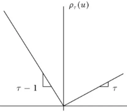
Figure 1.1: Check function used in the frequentist approach to quantile regression

coefficients vectorβ_τ can be estimated, in the frequentist approach, as the solution to min βτ T X t=i ρτ(yt−xtβτ) (1.2) where ρτ(u) = τ u if u≥0 −(1−τ)u if u <0, (1.3) which, graphically, assumes the form depicted in figure1.1.

As can be noted from the figure, the empirical check function is not dif-ferentiable at 0. As a consequence, the minimization of1.2can be achieved through an algorithm proposed by Koenker and D’Orey (1987) since a closed-form solution is not available.

Moreover, as observed by Koenker and Machado (1999), maximising the likelihood of the Asymmetric Laplace Distribution (ALD) is closely related to minimizing the empirical check function (1.2). In particular, a random variableu has an ALD(µ, σ, τ) with µ= 0,σ >0 and 0 < τ <1 if its pdf is given by

f(u;µ= 0, σ, τ) =τ(1−τ)

σ exp{−ρτ(u)} (1.4) whereµandσare the location and the scale parameters respectively and τ is the skewness parameter which is related with the location parameter in a particular way that allows us to use the ALD for quantile regression

(7)

models. Specifically, theτ-level quantile corresponds to the natural location parameter, i.e. P(u≤µ) =τ, therefore for a given value ofτ the estimate of µrepresents an estimate of theτ-level quantile for u.

Using this property, Yu and Moyeed (2001) suggested a Bayesian Quantile Regression approach using the ALD as likelihood tool. After the paper of Yu and Moyeed (2001) a wide Bayesian literature followed. Yu et al. (2007) develop a Bayesian framework for Tobit quantile regression and Kobayashi (2017) extended it to accounts for endogeneity. Santos and Bolfarine (2015) propose the use of Bayesian quantile regression for the analysis of response variables limited to the range (0,1), making use of the ALD in the likelihood calculation. Lum and Gelfand (2012) introduce the asymmetric Laplace process for quantile regression with spatially dependent errors. Reich et al. (2011) develop a Bayesian spatial quantile method for tropospheric ozone accounting for spatial variability by modeling the conditional distribution as a spatial process. Yue and Rue (2011) present a Bayesian quantile infer-ence method based on the integrated nested Laplace approximations (INLA) in additive mixed models assigning appropriate Gaussian Markov random field (GMRF) priors to different types of covariate. Hallin et al. (2010) present a multivariate extension of quantile based on a directional version of Koenker and Bassett’s traditional regression quantile using the L1 opti-mization ideas. Wang et al. (2016) introduce a quantile structural equation model to provide a comprehensive analysis of the interrelationships among latent variables still using the ALD. Kottas and Genlfand (2001) and Kot-tas and Krnjajic (2009) propose a Bayesian semiparametric methodology for quantile regression modelling. Hu et al. (2015) introduce a Bayesian quantile regression method for partially linear additive models which explic-itly models components that have linear and nonlinear effects while Chen and Yu (2009) propose a nonparametric quantile regression framework us-ing piecewise polynomial functions with number and location of knots in-ferred through reversible jump Markov chain Monte Carlo. Nonparametric Bayesian quantile regression is also considered in Thomson et al. (2010) that propose to model the dependence of a quantile of one variable on the values of another using a natural cubic spline. Sriram et al. (2013) provide justification for assuming ALD for the response in Bayesian Quantile Re-gression, even if it can represents a misspecification. Empirical likelihood as a working likelihood for quantile regression in Bayesian quantile infer-ence is considered in Yang and He (2012) while an approach based on the pseudo-joint Asymmetric Laplace Likelihood is implemented in Sriram et all. (2016). Novel application of quantile regression in the risk measure field is considered in Bernardi et al. (2015) and Meligkotsidou et al. (2009).

(8)

-2 -1 0 1 2 3 4 5 -2 -1 0 1 2 3 4 5 6 7 8

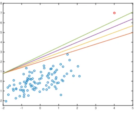
Figure 1.2: The robustness problem in quantile regression analysis

Finally, the problem of variable selection in Bayesian quantile regression models based on the ALD is considered in Yu et al. (2013), Alhamzawi and Yu (2012) (2015), Alhamzawi (2016), Ji et al. (2012).

Although the ALD is widely used in the Bayesian framework, its main disadvantage is displaying medium tails. This may produce misleading in-formation when extreme quantiles are concerned, and in particular, when the data are characterized by the presence of outliers and heavy tails. Ab-sence of a parameter governing tail fatness in the ALD may influence the final inference. Recently, Wichitaksorn et al. (2014) tried to generalize the classical Bayesian quantile regression by using some skew distributions, obtained through a mixture of scaled Normal ones. This class of distribu-tions allows for different degrees of asymmetry of the response variable also imposing a given structure of the tails.

To provide an idea about the robustness problem that may arise in quan-tile regression analysis let consider the case displayed in figure1.2in which we have a set of 100 observations characterized by the presence of the red colored outlier. All the plotted lines are just examples of lines which are compatible with the definition of quantile at τ = 0.99 (since they correctly leave the 99% of observations below) but among them we can observe that the red one is the most conservative. In this case, Bayesian quantile regres-sion based on the ALD tends to estimate a quantile function near to the green line while our goal is to estimate a quantile function as nearest as possible to the red line.

To overcome this drawback, we propose an extension of the Bayesian quantile regression by using the Skew Exponential Power (SEP) distribution

(9)

proposed in Zhu and Zinde–Walsh (2009). A useful property of the SEP distribution, similar to the ALD, is that the natural location parameter coincides with the τ-level quantile. Differently from the ALD, the SEP distribution also has a shape parameter governing the decay of the tails. Using the SEP distribution in quantile regression we are able to increase robustness of the inference, in particular when outliers or extreme values are present. One of the potential drawback of the SEP may be that it has one more parameter to estimate than ALD, so the estimation error/variation of this additional parameter may have effect on the quantile regression fitting, beside additional estimating burden. After all, this parameter is crucial to control the decay of the tails. In chapter2we show that, for all the estimated parameters, the chain rapidly converges toward the target distribution. In linear regression analysis several works have extensively considered the non-skewed version of the SEP, i.e. the Exponential Power distribution (EP), for its related robustness properties given by the shape parameter. Box and Tiao (1973) first show how to increase robustness of the classical Gaussian linear regression model, introducing the EP as a distribution assumption for the error term. Choy and Smith (1997), explore the robustness properties of posterior moments based on the EP distribution. Choy and Walker (2003) present further extension of the work of Choy and Smith (1997) proposing a case in which the shape parameter assumes values greater than two. Finally, Naranjo et al. (2015) and Kobayashi (2016) suggest the use of the SEP distribution in regression and stochastic volatility models. To the best of our knowledge, this thesis is the first attempt to improve robustness of quantile regression analysis by using the SEP distribution. In chapter 2 linear and Additive Models (AM) with penalized spline are considered to show the flexibility of the SEP in the Bayesian quantile regression context. Moreover, Lasso priors are considered in both cases to account for shrinking parameters problem when the parameters space becomes wide.

1.2 Quantile regression and risk measures

The interest towards a robust model for the conditional quantile function is primary in many fields, particularly in finance, where much attention is posed on methods and models for market risk measurement. Indeed, ac-curate risk measurement is a primary need for financial institutions and investors especially after the recent financial crisis. Within the instru-ments for market risk measurement, Value–at–Risk (VaR) (Jorion, 2007) and Expected Shortfall (ES) (Artzner et al, 1999) are certainly the most

(10)

popular and used approaches. VaR answers the question on what is the maximum potential loss that will be exceeded with a certain probability in the next days. Therefore, it can be simply understood as a specific con-ditional quantile of the portfolio returns given the current information i.e.

P(Yt<−VaRt| Ft) =τ, where Yt and Ft denote respectively the return of

a portfolio and the information set available at time t, while τ∈(0,1) de-notes the quantile confidence level associated with the VaR. Even though it is widely used among financial institutions VaR has been criticized because of the absence of the sub-additivity property, namely it does not guarantee that diversified portfolio is less risky than concentrated one. Artzner et al (1999) first recognize this lack of coherency of the VaR and proposed the ES as a possible alternative coherent risk measure which give more infor-mation about the distribution of returns in the tails. In particular the ES is defined as the conditional expected loss given that the loss exceed the VaR, i.e. E(Yt|yt<−VaR). But even if ES is a coherent risk measure it

is in general more difficult to backtest it, namely, to verify how accurately the strategy or method would have predicted actual results. Moreover, it is not as simple to interpret as the VaR and for these reasons there is not a prevailing risk measure between VaR and ES.

In literature there are several ways to estimate the VaR and the ES, some of them relying on distributional assumptions and some of them just estimate them directly. One of the recent approach is based on assuming conditional autoregressive equation structure, see for example Engle and Manganelli (2004) and Taylor (2008). In chapter 3 of this thesis we focus our atten-tion on the Condiatten-tional Autoregressive Value–At–Risk (CAViaR) class of models, introduced by Engle and Manganelli (2004), which belongs to the family of dynamic quantile autoregressive models proposed by Koenker et al. (2006), and the Conditional Autoregressive Expectile (CARE) class of models introduced by Taylor (2008).

The inferential issue for the CAViaR and the CARE class of models has been addressed in literature both from the frequentist and the Bayesian point of view. In the frequentist approach the CAViaR models allow to use the inferential quantile regression methods (Koenker, 2005) by minimizing the loss function introduced by Koenker and Basset (1978) and showed in the previous section (i.e. equation (1.2)). As explained before, the Bayesian approach instead relies on the Asymmetric Laplace distribution (ALD) as-sumption as a likelihood tool to perform the inferential issue (see e.g. Yu and Moyeed, 2001, Kottas and Gelfand, 2001, Kottas and Krnjajic, 2009, and Sriram et al.,2013, Bernardi et al., 2015).

(11)

the inferential strategy is instead based on the relation between expectile, quantile and ES (see Newey and Powell,1987). In particular, the estimation relies on the one-to-one mapping from expectiles to quantiles, and the rela-tionship between VaR and ES. In fact following Efron (1991), the estimator of theτ−thquantile will be theθ−thexpectile for which the proportion of observations below it is τ%, then the one–to–one mapping from expectiles to quantiles is used to obtain VaR and ES using equation (3.8) of Section 2 in chapter3. The estimation procedure for the generic expectile is addressed in the frequentist approach by using the Asymmetric Least Square (ALS) estimator as in Newey and Powell (1987) while in the Bayesian paradigm the literature relies on the Asymmetric Gaussian distribution assumption (see e.g. Gerlach and Wang, 2015, Gerlach and Chen, 2014; Wichitaksorn et al, 2014; Gerlach et al,2016, Gerlach and Chen, 2016)

In this thesis we propose to extend existing literature on conditional autore-gressive risk measure. First of all, we develop a unified Bayesian Conditional Autoregressive Risk model (B-CARM) which encompass both the CAViaR and the CARE one as particular case, again by using the SEP likelihood tool. As a second result we propose a new Non–Linear and semi–parametric specification of the B-CARM class of models which uses Penalized Splines (see De Boor, 2001, Eliers et al.,1996, Lang and Brazger,2004) to estimate the relation between the quantile/expectile and the observed variables. The need for a model that allows for non-linearity without assuming any particu-lar restrictions is of clear interest in literature. Indeed, all the specifications of the CAViaR and the CARE models proposed so far emphasize the role of asymmetry and non–linearity in the relation between the observed variables and the current quantile or expectile level, but they all impose the form of this non linearity a priori (see Engle and Manganelli, 2004, Gerlach et al., 2011 and 2012, Chen et al., 2009 and 2012, Gelach and Chen, 2014). In chapter 3 we will show that the proposed semi–parametric approach al-lows to obtain different form of nonlinearity in the CAViaR and the CARE models without employ any previous assumption about its structure.

(12)

(13)

Chapter 2

Bayesian robust quantile

regression

2.1 Introduction

In this chapter we propose the SEP distribution to develop a Bayesian robust quantile regression framework. In particular due to the specific characteris-tics of the SEP distribution we will show how to estimate the quantile func-tion firstly via simple linear regression and secondly by the Additive Models (AM). For the latter, we adopt the Penalized Spline (P–Spline) approach to carry out statistical inference. The Bayesian paradigm is implemented by means of a new adaptive Metropolis MCMC sampling scheme, with a full set of informative priors. In particular, for the AM framework, the proposed algorithm turns into an Adaptive Metropolis within Gibbs MCMC, allowing an efficient estimate of the penalization parameter and the P–Spline coeffi-cients.

When dealing with model building the choice of appropriate predictors and consequently the variable selection issue plays an important role. Here we approach this problem, by considering the Bayesian version of Lasso penal-ization methodology introduced by Tibshirani (1996). In particular, for the linear quantile regression model, we assume as prior distribution on each regressor, the generalized version of the univariate independent Laplace dis-tribution by Park and Casella (2008), Hans (2009) and Alhamzawi et al. (2012). Using this prior we shrink each parameter separately. When dealing with AM, we generalize the Lang and Brezger (2004) second order random walk prior for the spline coefficients, assuming a multivariate Laplace distri-bution and accounting for a correlation structure among parameters. This

(14)

prior corresponds to the group lasso penalty of of Yuan and Lin (2006), Meier et al. (2008) and Li et al. (2010) which in the spline context is im-mediately interpreted as knots associated with each regressor.

To analyze the performance of the proposed models we perform simulation studies in which we control for the weight of the outliers, the number of the parameters, the shape of the regressors and the presence of heteroschedas-ticity. Furthermore, we analyze three common real datasets: the corrected version (see Li et al., 2010) of the Boston housing data, first analyzed by Harrison and Rubinfeld (1978); the Munich rental dataset with geoadditive spatial effects, considered in Rue and Held (2005) and Yue and Rue (2011) among others; and the Barro growth data, first studied by Barro and Sala i-Martin (1995) and then extended in the quantile regression framework by Koenker and Machado (1999). The models we propose introduce robustness, variable selection and non-linearity in the estimation process, providing a more flexible framework and a new interpretation of some regression coeffi-cients and, on average, lower posterior standard deviations.

The remainder of the chapter is organized as follows. In Section 2.2, we introduce the SEP distribution and discuss its properties relevant to model conditional quantiles as functions of exogenous covariates. In Sec-tion 2.3 we introduce the model specification and the MCMC algorithms proposed. In Section 2.4 we look at the non–linear extension of the linear quantile approach via AM. Section 2.5 explores the sampling performance of the proposed models through simulations. Section2.6discusses three well known empirical applications while Section2.7 concludes.

2.2 The Skewed Exponential Power distribution

Zhu and Zinde–Walsh (2009) have recently proposed a parametrization of the SEP distribution introduced by Fernandez and Steel (1998), particularly convenient when quantiles are the main concern.

Definition 2.2.1. A random variable Y ∈ R is said to be Skewed

Expo-nential Power distributed, i.e. Y ∼ SEP(µ, σ, α, τ), if its density has the following form: fSEP(y;µ, σ, α, τ) =    1 σκEP(α) exp n −_α1 µ₂−_{τ σ}yαo , if y≤µ 1 σκEP(α) exp n −_α1 ₂₍₁₋y−_τµ₎_σαo, if y > µ, (2.1)

(15)

-4 -2 0 2 4 0 0.2 0.4 0.6 0.8 1 _{α=1; τ=0.5} α=2; τ=0.5 α=0.5; τ=0.5 (a) -4 -2 0 2 4 0 0.2 0.4 0.6 0.8 1 _{α=1; τ=0.5} α=2; τ=0.2 α=0.5; τ=0.8 (b)

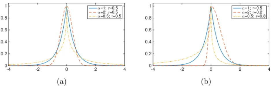
Figure 2.1: Plot of the SEP distribution for different level of the shape parameter (2.1(a)) and skewness parameter (2.1(b)) withσ= 1.0 andµ= 0.0.

and shape parameters respectively, while κEP=

h

2α1αΓ 1 + 1

α

i−1

withΓ (·)

is the complete gamma function. Moreover, the parameterτ ∈(0,1)controls for the skewness of the distribution.

We propose the use of (2.1) for quantile regression inference, as the lo-cation parameterµcoincides with theτ–level quantile (demonstrated in the gray box below). We also show (see Zhu and Zinde–Walsh, 2009) that the kurtosis of the SEP is directly determined by its parameterα. In Figure2.1 we present the pdf of the SEP distribution for different values of shape (α) and skewness (τ) parameters, with fixed values for the location and scale pa-rameters (µ, σ) = (0,1). It is worth noting that, for a fixed value of τ = 0.5 (see subfigure 2.1(a)), we retrieve the Laplace and the Normal distribution when the shape parameter is equal to α= 1 andα = 2, respectively. More-over, the smaller the value of α, the fatter the tails of the distribution and, in particular, asα →0 the SEP becomes the Chauchy distribution, while as α → ∞ it becomes equal to the Uniform distribution. Hence, it is evident that the parameter α is important in capturing the behavior of the tails, which may be fundamental when outliers or heavy tailed data are modelled. Furthermore, subfigure2.1(b)displays the behavior of the SEP for different combinations ofα and τ. In this case, the ALD (α = 1) and the Skew Nor-mal distribution (α= 2) can be obtained thanks to the skewness parameter τ. In the same figure, the relation between τ and the location parameterµ should also be noted. For a fixed µ(µ= 0 in the graph), by varying τ the shape of the distribution changes in such a way that µbecomes its quantile of level τ.

(16)

Lemma 2.2.1. Let Y ∼ SEP(µ, σ, α, τ), then the τ–level quantile of Y

coincides with its natural location parameter, i.e. Qτ(Y) =µ.

Proof. In order to show that P(Y ≤µ) =τ we compute the cdf of a SEP iny=µ P(Y ≤µ) = Z µ −∞ 1 2σ α−α1 Γ 1 +_α1 exp −1 α µ−y 2τ σ α 1(y≤µ) + exp −1 α y−µ 2 (1−τ)σ α 1(y>µ) dy = Z µ −∞ 1 2σ α−α1 Γ 1 +_α1exp −1 α µ−y 2τ σ α dy (2.2)

Without loss of generality, let us consider the case whenµ= 0 and σ = 1. The integral reduces to

α−α1 2Γ 1 + _α1 Z 0 −∞ exp −1 α ₋ y 2τ α dy. (2.3) By substitute (−y)α=xwe have α−α1 2Γ 1 +_α1 Z +∞ 0 exp − x α(2τ)α 1 α(x) 1 α−1_dx _(2.4)

Rearranging equation (2.4) and recognizing the kernel of a Gamma pdf with shape 1/αand scaleα(2τ)α the integral becomes

α−α1 2Γ 1 + _α1 1 αΓ 1 α (α(2τ)α)α1 _.

By using the property Γ(x+ 1) =xΓ(x) all the terms simplify except forτ, concluding the proof.

(17)

2.3 Robust Bayesian linear quantile regression

In this section we propose the use of the SEP distribution to implement the Bayesian inference for linear quantile regression combined with the prior distributions specification. Since we are interested in Lasso penalization problem in order to achieve sparsity within the quantile regression model, we propose as prior distribution for the regression parameters, a generalized version of the univariate independent Laplace distribution proposed by Park and Casella (2008) and Hans (2009). In line with Alhamzawi et al. (2012), for each quantile regression parameter we assume a Laplace distribution having different scale parameter in order to shrink each regression parameter in a different way. To achieve the Bayesian procedure we provide an adaptive MCMC sampling scheme obtained by running a block-move Independent Metropolis within Gibbs.

2.3.1 Model specification

Let Y = (Y1, Y2, . . . , YT) be a random sample of T observations, andXt =

(1, Xt,1, . . . , Xt,p−1)0, with t = 1,2, . . . , T equal to the associated set of p

covariates. Consider the following linear quantile regression model

Yt=X0tβτ +εt, t= 1,2, . . . , T, (2.5)

whereβτ = (βτ,0, βτ,1, . . . , βτ,p−1)0 is the vector ofpunknown regression pa-rameters, varying with the quantileτ level. Here, εt, for anyt= 1,2, . . . , T,

are independent random variables which are supposed to have zero τ–th quantile and constant variance. Assuming y= (y1, y2, . . . , yT) as a

realiza-tion of Y, andxtas a realization ofXt, then the likelihood function for the

model (2.5) based on the SEP distribution (2.1) with fixedτ can be written as: Lτ(βτ, σ, α,|y,xt) = T Y t=1 1 2σ α−α1 Γ 1 +_α1 exp −1 α x0_tβτ −yt 2τ σ α 1(yt≤x0tβτ) + exp −1 α yt−x0tβτ 2 (1−τ)σ α 1(yt>x0tβτ) = 1 (2σ)T α−Tα Γ 1 +_α1T " exp ( −1 α T X t=1 x0_tβτ−yt 2τ σ α) 1(yt≤x0tβτ) + exp ( −1 α T X t=1 yt−x0tβτ 2 (1−τ)σ α) 1(yt>x0tβτ) # , (2.6)

(18)

in this case the parameterµof equation (2.1) has been replaced by the re-gression functionµ=x0_tβ_τ. As discussed in the previous section, due to the property of the SEP distribution, the regression functionx0_tβ_τ corresponds to the conditional τ–level quantile of Yt, i.e. Qτ(Yt|Xt=xt) = x0tβτ. In

what follows, we omit the subscriptτ for the sake of simplicity.

The Bayesian inferential procedure requires the specification of the prior distribution for the unknown vector of parametersΞ= (β,γ, σ, α). As pre-viously mentioned, we generalize the prior proposed in Park and Casella for theβ parameter, assuming the hierarchical structure in (2.8) and (2.9); this allows efficient shrinkage of each parameter. The prior distribution is given by: π(Ξ) =π(β|γ)π(γ)π(σ)π(α), (2.7) with π(β|γ)∝ p Y j=1 L1(βj |0, γj) (2.8) π(γ)∝ p Y j=1 G(γj |ψ, $) (2.9) π(σ)∝ IG(a, b) (2.10) π(α)∝ B(c, d)1(0,2)(α), (2.11) whereβ∈_Rp_{. Here (}_{ψ, $, a, b, c, d}_{) are given positive hyperparameters and}

γ = (γ1, γ2, . . . , γp) are the parameters of the univariate Laplace

distribu-tion:

L1(βj |0, γj) =

γj

2 exp{−γj|βj|}1(−∞,+∞)(βj). (2.12) with zero location andγjscale parameter. In (2.9)-(2.11)G,IGandBdenote

the Gamma, Inverse Gamma and Beta distributions, respectively. Given its characteristics, the Laplace distribution is the Bayesian counterpart of the Lasso penalization methodology introduced by Tibshirani (1996) to achieve sparsity within the classical regression framework. The original Bayesian Lasso introduces the same univariate independent Laplace prior distribution for each regression parameter, see Park and Casella (2008) and Hans (2009). Here, as in Alhamzawi et al. (2012), we consider a more general case using the parameters γj,j = 1,2, . . . , p. By shrinking each regression parameter

in a different way, we overcome problems that may arise in the presence of regressors with different scales of measurement.

(19)

the Laplace distribution can be expressed as a location–scale mixture of Gaussians which, adapted to our case, becomes

L1(βj |0, γj) = Z ∞ 0 1 p 2πωj exp ( − β 2 j 2ωj ) γ_j2 2 exp ( −γ 2 jωj 2 ) dωj, (2.13)

for j = 1,2, . . . , p, where the mixing variable is exponentially distributed with shape parameter 2/γ_j2. Furthermore, to retain a parsimonious model parameterization, we introduce a second layer hierarchical prior represen-tation for the vector of shape parameters γ, in equation (2.9). Using the location–scale representation of the Laplace distribution, the prior structure defined in equations (2.8)–(2.9), can be represented as follows

β|ω∼ Np(β|0p,Ω) (2.14)

ωj |γj ∼ E ωj |2/γj2

(2.15) γj ∼ G(γj |ψ, $), (2.16)

where 0p is a column vector of zeros of dimension p, ω= (ω1, ω2, . . . , ωp)0,

Ω= diag{ωj, j = 1,2, . . . , p}andE is the exponential distribution. To

spec-ify values for the hyperparameters of the prior distributions, vague priors are typically imposed on the scaleσ, as it is viewed as a nuisance parameter, see e.g. Yu and Moyeed (2001) and Tokdar and Kadane (2012). We specify the prior for the shape parameter α by imposing a Beta distribution where c = 2 and d= 2. This allows for a large prior variance avoiding the prob-lem of U–shaped Beta distribution that would cause large probability mass to extreme values. In addition, we extend the Beta distribution to include the case of α ∈ (0,2) where α = 2 allows consideration of the so called conditional “expectile” of Newey and Powell (1987), while α = 1 allows consideration of conditional quantiles based on the ALD introduced by Yu and Moyeed (2001). The parameterα regulates the tail–fatness of the SEP distribution so that smaller values imply larger probabilities of extreme ob-servations (see Section 2.2). Therefore, by choosing α∈(0,2) we overcome both quantile and expectile regression issues, and we improve robustness by relying on a distribution with fatter tails than the Skew Normal.

In the following Section, we introduce the Bayesian parameter estimation procedure which aims to obtain simulations from the posterior distribution, using an Adaptive Independent Metropolis–Hastings MCMC algorithm.

(20)

2.3.2 Adaptive IMG for linear quantile regression

The Bayesian inference is carried out using an adaptive MCMC sampling scheme based on the following posterior distribution

π(Ξ|y,x)∝ Lτ(β, σ, α|y,x)π(β|γ)π(γ)π(σ)π(α), (2.17)

where L_τ(β, σ, α|y,x) indicates the likelihood function specified in equa-tion (3.17). After choosing a set of initial values for the parameter vector

Ξ(0), a block–move Independent Metropolis within Gibbs (IMG) is run it-eratively to obtain simulations from the posterior distribution at the i–th iteration of Ξ(i)_{, for} _i_{= 1}_,₂_{, . . .}_{. As a first step, the simulation algorithm} requires a proposal distribution for the parameters (β, σ, α).

We choose the following proposal distributions to move each block of the parameters: q(β)∼ Np β|µ(_βi),Σ(_βi) (2.18) q(σ)∼ N1 ˜ σ|µ(_σ_˜i), ψ_σ(_˜i) ∂σ˜ ∂σ (2.19) q(α)∼ N1 µ(_αi), ψ(_αi) 1(0,2)(α), (2.20) where the scale parameter ˜σ= log (σ) is considered on a log–scale and subse-quently transformed to preserve positive values. The jacobian term in equa-tion (3.28) is required for the distribution of the transformationσ= exp (˜σ). At each iterationi, the IMG algorithm draws a candidate parameter from each parameter block, i.e. Υ∗ = (ξ∗₁, ξ₂∗, ξ₃∗) = (β∗, σ∗, α∗) which is subse-quently accepted or rejected. The probability that the candidate parameter ξ∗_j, forj= 1,2,3 becomes the new state parameter of the chain is evaluated on the basis of the following acceptance probability

λξ_j(i−1), ξ∗_j= min    1, Lξ_j∗,Ξ₋(i−1)_j |y,x L Ξ(i−1)_|_y_,_x πξ_j∗ πξ(_ji−1) qξ(_ji−1) qξ∗_j    ,

forj= 1,2,3, whereλξ(_ji−1), ξ_j∗indicates the probability of moving to the new state of the chain,π(·) is the prior given in equations (2.8) - (2.11) and

Ξ(₋i−1)_j refers to the whole set of parameters at iteration i−1 without the j–th element of Υ∗. In the last step of the algorithm we sample (ωj, γj), for

(21)

full conditional distributions ωj |βj(i), γ (i−1) j ∼ GIG ωj 1 2, β (i) j 2 , γ_j(i−1)2 γ_j2(i)|ω_j(i)∼ G γ_j2 ψ+ 1, $+ ω(_ji) 2 ! .

where GIG denotes the Generalized Inverse Gaussian distribution. Since most of the statistical properties of the Markov chain, as well as the perfor-mance of the Monte Carlo estimators, depend crucially on the definition of the proposal distributionq(·) (see Andrieu and Moulines,2006and Andrieu and Thoms, 2008), we improve the basic IMG–MCMC algorithm with an additional step adapting the proposal parameters using the following equa-tions: µ(_βi+1) =µ(_βi)+ς(i+1) β−µ(_βi) , (2.21) Σ(_βi+1) =Σ(_βi)+ς(i+1) β−µ(_βi) β−µ(_βi) 0 −Σ(_βi) , (2.22) µ(_σ_˜i+1) =µ(_σ_˜i)+ς(i+1)σ˜−µ(_˜_σi), (2.23) ψ_σ_˜(i+1) =ψ_˜(_σi)+ς(i+1) ˜ σ−µ(_σ_˜i) 2 −ψ_σ(_˜i) , (2.24) µ(_αi+1) =µ(_αi)+ς(i+1) α−µ(_αi) , (2.25) ψ_α(i+1) =ψ(_αi)+ς(i+1) α−µ(_αi)2−ψ_α(i) , (2.26)

whereς(i+1) denotes a tuning parameter that should be carefully selected at each iteration to ensure the convergence and the ergodicity of the resulting chain (see Andrieu and Moulines, 2006). Roberts and Rosenthal (2007) provide two conditions for the convergence of the chain: the diminishing adaptation condition, which is satisfied if and only if ς(i)−→0, as i→+∞, and the bounded convergence condition, which guarantees that all transition kernels considered have bounded convergence time. Andrieu and Moulines (2006) show that both conditions are satisfied if and only ifς(i) ∝i−dwhere d ∈ [0.5,1]. Given this, we choose ς(i) = _Ci10.5 where C = 10. As argued by Roberts and Rosenthal (2007), these two conditions together ensure for this algorithm asymptotic convergence and a weak law of large numbers respectively.

(22)

2.4 Nonlinear extension

In this section, we propose an additive extension of the robust linear quantile regression model to the class of Additive Models (AM) introduced by Hastie and Tibshirani (1986). We set up AM using the SEP likelihood. In order to define the quantile function, we make use of the P-Spline functions resulting in a semiparametric problem. The Bayesian analysis is carried out by gener-alizing the Lang and Brezger (2004) second order random walk prior for the Spline coefficients, assuming a multivariate Laplace distribution. By doing so we account for a correlation structure among parameters which consider the issue of selection variables.

2.4.1 Non–linear model specification

AM extend multiple linear regression by allowing for the response variable to be modeled as sum of unknown smooth functions of continuous covariates. In this section we set up a robust non linear and semi–parametric framework for quantile regression following a AM approach using the SEP likelihood. In particular, we assume that theτ–level conditional quantile can be modeled as a parametric component jointly with a sum of smooth functions as follows:

Qτ(Yt|Xt=xt,Zt=zt) =x0tβ+ J

X

j=1

fj(zj,t), (2.27)

wherex0_tβis the parametric component, while eachfj(zj,t) is a

nonparamet-ric continuous smooth function andzt= (z1,t, z2,t, . . . , zJ,t)0 is an additional

set of covariates. To implement the statistical analysis we assume that the non-parametric componentfj(ztj) can be approximated using a polynomial

spline of order d, with k + 1 equally spaced knots between min (zt) and

max (zt). Using the well known representation of splines in terms of linear

combinations of B–splines, we can rewrite equation (2.27) as:

Qτ(Yt|Xt=xt,Zt=zt) =x0tβ+ J X j=1 k+d X ν=1 θj,νBj,ν(ztj), (2.28)

where Bj,ν(ztj) denote B–spline basis functions and θj,ν are the unknown

coefficients. In this framework, the value of the estimated coefficients and the shape of the fitted functions strongly depend upon the number and the position of the knots. With respect to the position, in the absence of prior information, we consider equidistant knots as the natural choice. To prop-erly capture the smoothness of the data, careful consideration must be given

(23)

to the trade-off between too few and too many knots, which may cause un-derfitting or overfitting respectively. A possible solution to this problem is known as Penalized Spline (P–Spline) proposed by O’Sullivan (1986 and

1988) and generalized by Eilers and Marx (1996), which relies on the intro-duction of a penalty element on the first or second differences of the B–Spline coefficients. This setting has been embedded in the Bayesian framework by Lang and Brezger (2004), Brezger and Lang (2006) and Brezger and Steiner (2008) using a second order random walk for all the B–Spline coefficients, i.e.:

θj,ν = 2θj,ν−1−θj,ν−2+uj,ν, ∀j= 1,2, . . . , J, ∀ν = 1,2, . . . , k+d,

(2.29) where the generic stochastic component uj,ν ∼ N(0, hj), θj,1 and θj,2 are initialized with diffuse priors, i.e., π(θj,ν) ∝1, for ν = 1,2. In their work

Lang and Brezger (2004) assume that the stochastic componentsuj,ν driving

the random walk process are independent, i.e. uj,ν ⊥ uk,ν, for all j, k =

1,2, . . . , J with j 6= k. As there are no reasons to assume a priori uj,ν

and uk,ν as being independent (∀j, k), we consider an extension of (2.29)

and assume a multivariate Laplace distribution on the vector of regressors accounting for a correlation structure amongst them. It can be showed that, under the assumed prior structure, the original marginal shrinkage effect is preserved because each marginal prior reduces to a univariate Laplace, see, e.g., Kotz et al. (2001).

Moreover, using the Laplace distribution as prior distribution allows the extension of the Lasso approach to the Bayesian paradigm.

Letuj = (uj,1, uj,2, . . . , uj,k+d), we assume uj ∼ ALk+d(0,Ik+d), where

ALk+ddenotes the multivariate Laplace distribution andId+kis the identity

matrix of dimensionk+d. Furthermore, let Dδ be the difference matrix of

dimension (k+d−δ)×(k+d), and δ = 2 is the order of the differential operator, such that Dδθj =uj, then

π(θj |hj)∼ ALk+d 0, hj D0δDδ , ∀j= 1,2, . . . , J, (2.30) having density π(θj |hj) =C|D0δDδ| 1 2hd+k j exp n −hj θ0_j D0_δDδ θj 1₂o , (2.31) where C = √ 2π Γ(d+k+1 2 )

. As shown in Kotz et al. (2001), the multivariate Laplace distribution can be expressed as a location–scale mixture of

(24)

Gaus-sians, where the mixing variable follows a Gamma distribution π(θj |φj)∼ Nk+d 0, φj D0δDδ −1 (2.32) π(φj |hj)∼ G k+d+ 1 2 , h2_j 2 ! , (2.33) forj= 1,2, . . . , J.

It can easily be shown how to retrieve (2.31) from (2.32) - (2.33) by inte-grating out the augmented variableφj, i.e.

π(θj |hj) = Z R |D0_δDδ| 1 2 exp −θ 0₍_D0 δDδ)θ 2φj (2πφj) k+d 2 h2_j 2 d+k₂+1 φ d+k−1 2 j Γ d+k₂+1 ×exp ( −h2_jφj 2 ) dφj = h2 j 2 d+k₂+1 |D0_δDδ| 1 2 (2π)k+2d_Γ d+k+1 2 × Z R φ− 1 2 j exp −1 2 θ0(D0_δDδ)θ φj +h2_jφj dφj, (2.34) where the integrand in the previous equation (2.34) is proportional to a Generalized Inverse Gaussian distributionGIG(p, a, b) with parametersp= 1 2,a=h 2 j and b=θ 0 j(D 0

δDδ)θj from which we have

Z R φ− 1 2 j exp −1 2 θ0(D0_δDδ)θ φj +h2_jφj dφj = 2K1 2 r h2 j θ0_j D0_δDδ θj h2 j θ0 j(D0δDδ)θj 1₄ , (2.35) whereK1 2(z) = p_π 2zexp{−z}.

(25)

Substituting this latter expression into equation (2.34) we obtain π(θj |hj) = h2 j 2 d+k₂+1 |D0_δDδ| 1 2 (2π)k+2d_Γ d+k+1 2 √ 2πexpn−hj q θ0 j(D 0 δDδ)θj o [h2 j(θ 0 j(D 0 δDδ)θj)] 1 4 h2 j θ0_j(D0_δDδ)θj 1₄ = √ π|D0_δDδ| 1 2hd+k j Γ d+k₂+1 exp n −hj q θ0_j D0_δDδ θj o , (2.36) which corresponds to the ALD defined in equations (2.30)–(2.31). The pro-posed prior distribution for θj corresponds to the group lasso penalty of

Yuan and Lin (2006), Meier et al. (2008) and Li et al. (2010), account-ing for the group structure when performaccount-ing variable selection. It is worth emphasizing that, in our context, the group variables have a natural inter-pretation because they correspond to knots accounting for the smoothness level of the same regressor over different regions of the support. The overall smoothness of the fitted curve is controlled by the variance of the error term hj, and this corresponds to the inverse of the penalization parameter used

by Eilers et al. (1996) in the frequentist framework. We choose a conjugate Gamma prior for h2

j, that is h2j ∼ G a(h), b(h)

witha(h) ₌_b(h) _{= 0}_._{001. A} different choice of hyperparameters may be considered, however, they may all bring very similar results. To sum up, the use of a Gamma prior for h2_j, and the assumption of the prior structure defined in equations (2.8)–(2.9) for the shape and scale parameters (σ, α), provides the following hierarchical model yt=x0tβ+ J X j=1 Bz_jθj+t, t∼ SEP(0, τ, σ, α) (2.37) β|ω∼ N_p(β|0p,Ω) (2.38) ωk|γk∼ E ωk|2/γk2 (2.39) γk∼ G(γk|ψ, $), ∀k= 1,2, . . . , p (2.40) θj |φj ∼ Nk+d 0, φj D0δDδ −1 (2.41) φj |hj ∼ G d+k+ 1 2 , h2 j 2 ! (2.42) h2_j ∼ IG a (h) 2 , b(h) 2 ! ∀j= 1,2, . . . , J, (2.43)

(26)

whereBz_j = (Bj,1(ztj), . . . , Bj,k+d(ztj)).

2.4.2 Adaptive IMG for quantiles AM

In order to perform the Bayesian inference, the Adaptive MCMC algorithm proposed in Section2.3.2is slightly modified to deal with the simulation from the posterior distribution of the generalized quantiles’ AM parameters. The posterior distribution becomes equal to

π(Ξ|y,x,z)∝ L_τ(β, σ, α,ϑ|y,x,z)π(β|γ)π(γ)

×π(ϑ|φ)π(φ|h)π(h)π(σ, α) (2.44) where the vector Ξ now contains an additional three sets of parameters, namely ϑ= (θ1,θ2, . . . ,θJ),φ= (φ1, φ2, . . . , φJ) and h= h21, h22, . . . , h2J

. The likelihood functionLτ(β, σ, α,ϑ|y,x,z) defined in equation (3.17) for

the linear model, should be adapted to account for the additional spline coefficients. In order to perform Bayesian analysis, three additional steps to the algorithm described in Section2.3.2are required. In particular, having updated all the parameters of the linear part of the model, a candidate for θj, for j = 1,2, . . . , J is drawn from a Gaussian proposal distribution, i.e.,

qθj,i−1, θ∗_j ∼ N_k₊_dµ(_θi) j,Σ (i) θj

and accepted on the basis of the following acceptance probability λ θ(_ji−1),θ∗_j = min    1, Lβ(i−1), σ(i−1), α(i−1),θ_j∗,ϑ(₋i−1)_j |y,x,z Lβ(i−1)_{, σ}(i−1)_{, α}(i−1)_,_ϑ(i−1) j |y,x,z × πθ_j∗ πθ_j(i−1) qθ_j(i−1) qθ_j∗    ,

where ϑ−j denote the whole set of B–Spline coefficients without the j–

th component. Furthermore, as specified for the regression parameters in Section2.3.2, an adaptive step for the mean and the variance of the proposal distribution of eachθj is implemented using the following equation

µ(_θi+1) j =µ (i) θj +ς (i+1)_θ j −µ(_θi_j) , (2.45) Σ(_θi+1) j =Σ (i) θj +ς (i+1) θj−µ(_θi_j) θj−µ(_θi_j) 0 −Σ(_θi) j , (2.46)

(27)

forj= 1,2, . . . , J, whereς is the vanishing factor, fixed as discussed above. The hyperparameters (φ,h) are updated by single–move Gibbs sampling steps, by simulating from the following full conditionals which are propor-tional to the GIG distribution

φj |θj(i), h (i−1) j ∼ GIG φj 1 2, h (i−1) j 2 ,θ_j0 D0_δDδ θj h2_j |φ(_ji)∼ GIG h2_j − ah 2 , φ (i) j , bh 2 .

2.5 Simulation Studies

We perform simulation studies to highlight the improvements in robustness obtained by implementing SEP-based quantile regression, compared with that obtained by the traditional Bayesian quantile regression, based on the ADL distribution. Our purpose is to illustrate how the SEP misspecified model assumption in the quantile regression framework generates posterior distributions of the regression parameters centered on the true values. The first simulation experiment assesses the robustness properties of the pro-posed methodology for quantile estimation when the joint distribution of the couple (Yi,Xi), for i = 1,2, . . . , T, is contaminated by the presence of

outliers. The second study shows the effectiveness of the shrinkage effect, obtained by imposing the Lasso–type prior, used when the multiple quantile linear model is of key concern. The last experiment aims at highlighting the ability of the model to adapt to non–linear shapes, when data come from heterogeneous fat–tailed distributions. The hyperparameters of the prior distributions are chosen such that the priors are non-informative. In particular, for the nuisance parameter σ we choose a = b = 0.001 which corresponds to a proper Inverse Gamma distribution with infinite second moments. When lasso prior is assumed, the hyperparameters (ψ, $) in the Gamma priors for γj are set at 0.1.

2.5.1 Simple linear quantile regression

For this experiment we consider a sample of T = 100 drawn from the following homoskedastic mixture of distributions

f (Y, X)0,η,µ₁,µ₂, . . . ,µ_L,Σ=

L

X

l=1

(28)

-3 -2 -1 0 1 2 3 -4 -2 0 2 4 6 8 (a)τ= 0.1, T = 100 -3 -2 -1 0 1 2 3 -4 -2 0 2 4 6 8 (b) τ= 0.5, T = 100 -3 -2 -1 0 1 2 3 -4 -2 0 2 4 6 8 (c)τ = 0.9, T = 100

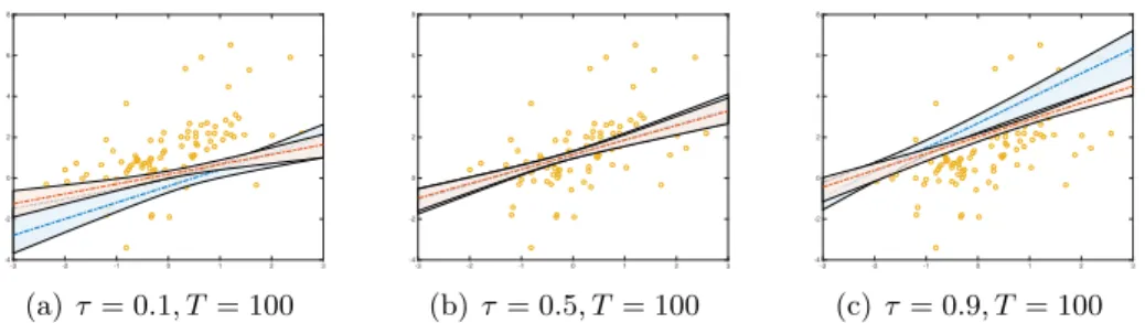
Figure 2.2: Contaminated data example. Comparison between Bayesian quantile re-gression based on the ALD (blue) and the SEP distribution (red) for different values of the quantile confidence levelτ = (0.1,0.5,0.9) and sample sizesT = 100. Shaded areas denote 95% HPD credible sets.

whereϕdenotes the density function of a Gaussian distribution with mean µand variance and covariance matrixΣ, andη= (η1,· · ·, ηL) is the vector

of weights. We set the number of components equal toL= 3, with mixture weightsη= (0.85,0.0725,0.0725), locations and scale matrix specified as

µ₁ = 1 0 , µ₂ = 4 0 , µ₃= −2 0 , Σ= 1 0.6 0.6 1 . (2.48) The quantile regression model used is a simple model with only one exoge-nous variable i.e. Yt=Xtβ+εtfort= 1,2, . . . T. The aim of this example is

to show the performance of the Bayesian quantile linear regression analysis assuming both the ALD and the SEP likelihood when the data are strongly contaminated by the presence of outliers. Since we have only one regres-sor, for this example we use a simplified version of the sampler proposed in Section2.3.2, in which a simple Gaussian prior is considered for β. For τ = (0.1,0.5,0.9) we run the MCMC algorithm with N = 50,000 iterations and a burn–in of M = 10,000. For both the ALD and the SEP distribu-tion assumpdistribu-tions, initial values for the parameters to be estimated, namely (β, σ), are randomly drawn fromN(0,1) andIG(0.001,0.001), respectively. The additional initial value for the parameterα, required only for the SEP distribution case, is randomly drawn formB(2,2).

Figure2.2depicts the estimated regression lines as well as the 95% HPD credible sets. The blue line refers to the ALD estimation while the red line to the SEP one. It can be easily observed that the two curves overlap for τ = 0.5 and diverge increasingly for extreme level quantiles i.e. for τ = (0.1,0.9). In the case thatτ = 0.5 the posterior mean ofα is very close to one, implying that the SEP reduces to the ALD distribution.

(29)

Parameter ALD SEP τ = 0.1 τ = 0.5 τ = 0.9 τ = 0.1 τ = 0.5 τ = 0.9 β0 -0.391 1.149 2.688 0.186 1.144 2.011 (0.176) (0.093) (0.237) (0.089) (0.086) (0.100) β1 0.801 0.735 1.207 0.428 0.709 0.825 (0.151) (0.106) (0.144) (0.094) (0.093) (0.074) σ 3.844 2.105 3.478 1.049 0.862 0.989 (0.386) (0.212) (0.349) (0.153) (0.112) (0.150) α - - - 0.596 0.832 0.504 (0.094) (0.142) (0.068)

Table 2.1: Contaminated data example. Estimated parameters for different levels of the quantile confidence level τ = (0.1,0.5,0.9) and T = 100. Standard deviations in parenthesis.

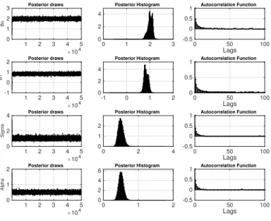
The further we move away from the median, the more e the differences in the estimated regression quantile parameters under the ALD and the SEP assumptions are noticeable. When using the ALD distribution, the intercept and slope of the regression line are strongly influenced by the outliers (7.25% of the total observations) generated by the two external components of the mixture (2.2(a)and2.2(c)). In both cases, the estimated α of the SEP is considerably smaller than one. As a consequence estimation of the β parameters is made under a distribution with fatter tails than the ALD, strongly penalizing more extreme observations and providing us with more robust results. For the regression parameters, Table2.1 contains the estimated posterior means and standard deviations under the ALD and the SEP assumptions. In the data generating process, the theoretical slope should always be equal to 0.6. When moving from the median to more extreme quantiles, the ALD-estimated posterior mean of the intercept and the slope is farther from the true value than those obtained with the SEP. It is worth noting that the SEP standard errors are always lower, implying that the estimated parameters are sharper when using the SEP distribution. Finally, figures 2.3-2.5 provide evidence about the efficiency of the MCMC algorithm implemented by showing posterior draws, posterior histograms and Autocorrelation functions for the estimated SEP robust parameters for the three different values ofτ.

(30)

×104 1 2 3 4 5 Bo -0.5 0 0.5 1 Posterior draws -0.5 0 0.5 1 0 2 4 Posterior Histogram Lags 0 50 100 -0.5 0 0.5 1 Autocorrelation Function ×104 1 2 3 4 5 B1 0 1 2 Posterior draws 0 1 2 0 2 4 Posterior Histogram Lags 0 50 100 -0.5 0 0.5 1 Autocorrelation Function ×104 1 2 3 4 5 Sigma 0.5 1 1.5 2 Posterior draws 0.5 1 1.5 2 0 1 2 Posterior Histogram Lags 0 50 100 -0.5 0 0.5 1 Autocorrelation Function ×104 1 2 3 4 5 Alpha 0 0.5 1 Posterior draws 0 0.5 1 0 2 4 Posterior Histogram Lags 0 50 100 -0.5 0 0.5 1 Autocorrelation Function

Figure 2.3: Posterior draws, posterior histograms and ACF for estimated robust (SEP) parameters of simple linear quantile regression simulation withτ = 0.1

×104 1 2 3 4 5 Bo 0.5 1 1.5 2 Posterior draws 0.5 1 1.5 2 0 2 4 Posterior Histogram Lags 0 50 100 -0.5 0 0.5 1 Autocorrelation Function ×104 1 2 3 4 5 B1 0 0.5 1 1.5 Posterior draws 0 0.5 1 1.5 0 2 4 Posterior Histogram Lags 0 50 100 -0.5 0 0.5 1 Autocorrelation Function ×104 1 2 3 4 5 Sigma 0.5 1 1.5 Posterior draws 0.5 1 1.5 0 2 4 Posterior Histogram Lags 0 50 100 -0.5 0 0.5 1 Autocorrelation Function ×104 1 2 3 4 5 Alpha 0 0.5 1 1.5 Posterior draws 0 0.5 1 1.5 0 1 2 3 Posterior Histogram Lags 0 50 100 -0.5 0 0.5 1 Autocorrelation Function

Figure 2.4: Posterior draws, posterior histograms and ACF for estimated robust (SEP) parameters of simple linear quantile regression simulation withτ = 0.5

(31)

×104 1 2 3 4 5 Bo 0 1 2 3 Posterior draws 0 1 2 3 0 2 4 Posterior Histogram Lags 0 50 100 -0.5 0 0.5 1 Autocorrelation Function ×104 1 2 3 4 5 B1 -1 0 1 2 Posterior draws -1 0 1 2 0 2 4 Posterior Histogram Lags 0 50 100 0 0.5 1 Autocorrelation Function ×104 1 2 3 4 5 Sigma 0 2 4 Posterior draws 0 2 4 0 1 2 Posterior Histogram Lags 0 50 100 -0.5 0 0.5 1 Autocorrelation Function ×104 1 2 3 4 5 Alpha 0 1 2 Posterior draws 0 1 2 0 2 4 6 Posterior Histogram Lags 0 50 100 -0.5 0 0.5 1 Autocorrelation Function

Figure 2.5: Posterior draws, posterior histograms and ACF for estimated robust (SEP) parameters of simple linear quantile regression simulation withτ= 0.9

2.5.2 Multiple quantile regression

In this section, we carry out a Monte Carlo simulation study specifically tailored to evaluate the performance of the model when the Lasso prior (2.8) is considered for the regression parameters. The simulations are similar to the one proposed in Li et al. (2010) and Alhamzawi et al. (2012). In particular, we simulate T = 200 observations from the linear model Yt =

X0_tβ+εt, where the true values for the regressors are set as follows:

Simulation 1. β= (3,1.5,0,0,2,0,0,0)0,

Simulation 2. β= (0.85,0.85,0.85,0.85,0.85,0.85,0.85,0.85)0, Simulation 3. β= (5,0,0,0,0,0,0,0)0,

The first simulation corresponds to a sparse regression case, the second to a dense case, and the third to a very sparse case. The covariates are in-dependently generated from a N (0,Σ) with σi,j = 0.5|i−j|. Two different

distributions for the error terms generating process are considered for each simulation study. The first is a Gaussian distribution N µ, σ2, with µset so that the τ-th quantile is 0, while σ2 is set as 9, as in Li et al. (2010). The second distribution is a Generalized Student’t GS µ, σ2, ν

(32)

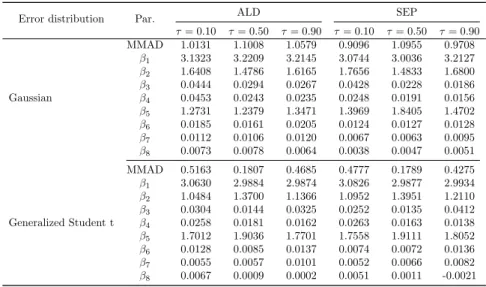
degrees of freedom, i.e. ν = 2, σ2 = 9 and µ set so that the τ-th quantile is 0. For three different quantile levels, τ = (0.10,0.5,0.9) we run 50 simu-lations for each vector of parameters (β) and each distribution of the error term. Table 2.2 reports the median of mean absolute deviation (MMAD), i.e. median 1 200 P200 t=1|x 0 tβˆ−x0tβ|

, and the median of the parameters β,ˆ over 50 estimates. Results for the first simulation are reported, since re-sults from the other two simulations are qualitatively similar. The proposed Bayesian quantile regression method based on the SEP likelihood performs better in terms of MMAD for both distributions of the error term. This is evidence that the presence of the shape parameterαin the likelihood better capture the behavior of the data. The estimated shape parameter is in-deed greater and lower than one in the Gaussian and Generalized Student’t cases, respectively; this provides a more reliable estimation of the vectorβ, regardless of the tail weight of the error term distribution. These results are reinforced in the second and third simulation (not reported here) in which we exaggerate the density and the sparsity of the predictors structure. Fur-thermore, the proposed robust method reduces the bias of estimated β for all quantile confidence levels. Regarding the shrinkage ability of the pro-posed estimator, when the true parameters are zero, the SEP distribution performs better than the ALD in identifying the parameters .

Error distribution Par. ALD SEP

τ= 0.10 τ= 0.50 τ= 0.90 τ= 0.10 τ= 0.50 τ= 0.90 Gaussian MMAD 1.0131 1.1008 1.0579 0.9096 1.0955 0.9708 β1 3.1323 3.2209 3.2145 3.0744 3.0036 3.2127 β2 1.6408 1.4786 1.6165 1.7656 1.4833 1.6800 β3 0.0444 0.0294 0.0267 0.0428 0.0228 0.0186 β4 0.0453 0.0243 0.0235 0.0248 0.0191 0.0156 β5 1.2731 1.2379 1.3471 1.3969 1.8405 1.4702 β6 0.0185 0.0161 0.0205 0.0124 0.0127 0.0128 β7 0.0112 0.0106 0.0120 0.0067 0.0063 0.0095 β8 0.0073 0.0078 0.0064 0.0038 0.0047 0.0051 Generalized Student t MMAD 0.5163 0.1807 0.4685 0.4777 0.1789 0.4275 β1 3.0630 2.9884 2.9874 3.0826 2.9877 2.9934 β2 1.0484 1.3700 1.1366 1.0952 1.3951 1.2110 β3 0.0304 0.0144 0.0325 0.0252 0.0135 0.0412 β4 0.0258 0.0181 0.0162 0.0263 0.0163 0.0138 β5 1.7012 1.9036 1.7701 1.7558 1.9111 1.8052 β6 0.0128 0.0085 0.0137 0.0074 0.0072 0.0136 β7 0.0055 0.0057 0.0101 0.0052 0.0066 0.0082 β8 0.0067 0.0009 0.0002 0.0051 0.0011 -0.0021

Table 2.2: Multiple regression simulated data example 1. MMADs and estimated pa-rameters for Simulation 1 under the SEP and ALD assumption for the quantile error term.

(33)

2.5.3 Non Linear Model

In this simulation example we illustrate how well the model assumptions perform when a simple AM is employed with a single continuous smooth non–linear function and where the parametric linear components are set to zero. Following Chen and Yu (2009), we consider two data generating processesyt=fj(xt)+t, fort= 1,2, . . . , T andj= 1,2 wheref1 represents the wave function andf2 the doppler function, defined as follows

f1(x) = 4 (x−0.5) + 2 exp −256 (x−0.5)2 1(0,1)(x) (2.49) f2(x) = (0.2x(1−0.2x)) 1 2_sin 2π(1 +γ) 0.2x+γ 1(0,1)(x), (2.50) with γ = 0.15. These functions are usually used (see also Denison et al.

1998) to check the nonlinear fitting ability of a model. Starting from these two curves, we generate a sample of T = 200 and T = 512 observations for the wave and the doppler functions respectively, using four different sources of error Gaussian noise, t∼ N(0,1) (2.51) yt=f1(xt) +σ1t, yt=f2(xt) +σ2t, Student–t noise, t∼ Tν(0,1), (2.52) yt=f1(xt) +σ1t, yt=f2(xt) +σ2t, Linear heterogeneity, t∼ Tν(0,1), (2.53) yt=f(xt) +σ1(1 +x)t, yt=f(xt) +σ2(1 +x)t, Quadratic heterogeneity, t∼ Tν(0,1), (2.54) yt=f1(xt) +σ1 1 +x2t t, yt=f2(xt) +σ2 1 +x2t t, where σ1 = √ 0.4, σ2 = √

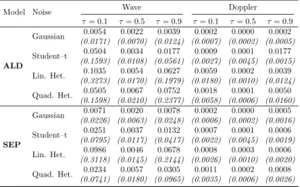
0.1 and ν = 2. The set of model specifications considered are estimated using penalized P–Splines of order 4. imposing a relatively large number of equally spaced knots and a penalization parameter δ = 2, as suggested by Eilers et al. (1996). In particular, we use 20 knots for the wave function and 25 knots for the doppler function due to the presence of many change points. The sampling process is performed using

(34)

Model Noise Wave Doppler τ= 0.1 τ= 0.5 τ= 0.9 τ= 0.1 τ= 0.5 τ= 0.9 ALD Gaussian 0.0054 0.0022 0.0039 0.0002 0.0000 0.0002 (0.0171) (0.0070) (0.0124) (0.0007) (0.0002) (0.0005) Student–t 0.0504 0.0034 0.0177 0.0009 0.0001 0.0177 (0.1593) (0.0108) (0.0561) (0.0027) (0.0045) (0.0015) Lin. Het. 0.1035 0.0054 0.0627 0.0059 0.0002 0.0039 (0.3273) (0.0170) (0.1979) (0.0180) (0.0010) (0.0124) Quad. Het. 0.0505 0.0067 0.0752 0.0018 0.0001 0.0050 (0.1598) (0.0210) (0.2377) (0.0058) (0.0006) (0.0160) SEP Gaussian 0.0071 0.0020 0.0078 0.0002 0.0000 0.0005 (0.0226) (0.0063) (0.0248) (0.0006) (0.0002) (0.0016) Student–t 0.0251 0.0037 0.0132 0.0007 0.0001 0.0006 (0.0795) (0.0117) (0.0417) (0.0022) (0.0045) (0.0019) Lin. Het. 0.0986 0.0046 0.0678 0.0008 0.0003 0.0006 (0.3118) (0.0145) (0.2144) (0.0026) (0.0010) (0.0020) Quad. Het. 0.0234 0.0057 0.0305 0.0011 0.0002 0.0008 (0.0741) (0.0180) (0.0965) (0.0035) (0.0006) (0.0026)

Table 2.3: Non–linear regression simulated data example. MSE of the fitted curves with four sources of noise evaluated over the 200 synthetic replications. Standard deviations in parenthesis.

50,000 iterations with the first 10,000 as burn–in. For all described curves, Table 2.3 shows the average and the standard errors of the mean squared errors (mse) of three different quantile levels (50 repeats) . It can be noted that the SEP outperforms the ALD in terms ofmse almost systematically. The difference between the two curves is less evident in the presence of Gaussian errors, where the ALD also displays a smallermse for the extreme quantiles of the wave function. The improvement in terms of estimation bias becomes larger when looking at more heavy tailed and heteroskedastic error distributions. Concerning the wave function, the SEP shows a mse equal to half of that obtained with the ALD at the extreme quantiles. The same conclusions can be drawn for the doppler function that is generally better estimated than the wave function.

2.6 Empirical applications

Three empirical datasets are analyzed in this section: Boston Housing, Mu-nich Rent and Barro growth data. The first dataset is characterized by the presence of many regressors that emphasizes the usefulness of introducing a lasso prior for the regression parameters. The second dataset also has a large set of regressors with some characterized by a non-linear relationship with the response variable. For this dataset we highlight that the

(35)

assump-tion of a lasso prior within a robust quantile AM framework leads to a more precise estimation process. Finally we propose the use of our robust quantile lasso AM to study the Barro growth data in a previously unexplored way by assuming a non linear representation for some regressors. We find a new interpretation of regression parameters while maintaining the neoclassical convergence hypothesis.

2.6.1 Boston housing data

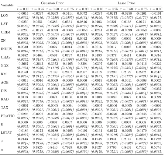
In this section we analyze the Boston Housing data first considered by Harrison and Rubinfeld (1978) studying the influence of pollution on house prices. In particular, in this section we consider the corrected data of Li et al. (2010). The model is based on the log-transformed corrected median values of owner-occupied housing (values in USD 1000) as the dependent variable while several exogenous variables are taken into account: the point longitudes and latitudes in decimal degrees (LON and LAT respectively); the per capita crime (CRIM); the proportions of residential land zoned and non-retail business acres per town (ZN and INDUS respectively); a dummy equal to 1 if tract borders Charles River (CHAS); the nitric oxide concentra-tion (NOX); the average number of rooms per dwelling (RM); the proporconcentra-tion of owner-occupied units built prior to 1940 (AGE); the weighted distances to five Boston employment centers (DIS); the index of accessibility to radial highways per town (RAD); the full-value property-tax rate per town (TAX); the pupil-teacher ratios per town (PTRATIO); the transformed Black pop-ulation proportion (B); and, percentage values of lower status poppop-ulation (LSTAT). To provide a description of the conditional distribution of the re-sponse variable we consider five values of τ, i.e. 0.10 0.25 0.50 0.75 0.90. Moreover, in order to show the advantage and performance of assuming a Lasso prior for the regressor parameters we also consider a Gaussian prior distribution. Results are reported in Table2.4. Independently of the choice of prior distribution, all variables have a sign similar to previous studies us-ing the same dataset. Nevertheless, the Lasso prior should be preferred for at least for two reasons. Firstly, it systematically provides smaller posterior standard errors. Secondly, the estimated coefficients appear to be more reli-able at extreme quantile levels, i.e. τ = 0.1 orτ = 0.9, where the estimated parameters obtained under Gaussian prior become very unstable for some variables.

(36)

Variable Gaussian Prior Lasso Prior τ= 0.10 τ= 0.25 τ= 0.50 τ= 0.75 τ= 0.90 τ= 0.10 τ= 0.25 τ= 0.50 τ= 0.75 τ= 0.90 LON -0.0614 -0.0297 -0.0203 -0.0114 0.0072 -0.0287 -0.0213 -0.0258 -0.0261 -0.0161 (0.0364) (0.0416) (0.0450) (0.0555) (0.0434) (0.0166) (0.0172) (0.0187) (0.0176) (0.0157) LAT -0.0250 0.0251 0.0386 0.0531 0.0816 0.0103 0.0221 0.0168 0.0121 0.0238 (0.0582) (0.0678) (0.0732) (0.0937) (0.0729) (0.0276) (0.0290) (0.0311) (0.0296) (0.0262) CRIM -0.0230 -0.0177 -0.0093 -0.0063 -0.0058 -0.0241 -0.0178 -0.0093 -0.0059 -0.0032 (0.0032) (0.0027) (0.0015) (0.0016) (0.0021) (0.0028) (0.0027) (0.0014) (0.0017) (0.0014) ZN 0.0000 0.0005 0.0008 0.0012 0.0012 -0.0000 0.0006 0.0009 0.0010 0.0009 (0.0003) (0.0003) (0.0004) (0.0004) (0.0003) (0.0003) (0.0003) (0.0004) (0.0003) (0.0002) INDUS 0.0030 0.0023 0.0027 0.0014 -0.0013 0.0016 0.0017 0.0016 0.0010 -0.0027 (0.0016) (0.0014) (0.0016) (0.0017) (0.0013) (0.0015) (0.0014) (0.0016) (0.0017) (0.0011) CHAS 0.0482 0.0464 0.0597 0.0737 0.1134 0.0183 0.0377 0.0411 0.0448 0.0834 (0.0264) (0.0197) (0.0264) (0.0308) (0.0302) (0.0190) (0.0205) (0.0236) (0.0275) (0.0312) NOX -0.3667 -0.2642 -0.3672 -0.4465 -0.3204 -0.0397 -0.0604 -0.0480 -0.0416 -0.0222 (0.1324) (0.0946) (0.1119) (0.1424) (0.1191) (0.0463) (0.0575) (0.0551) (0.0524) (0.0395) RM 0.2050 0.2259 0.2139 0.2007 0.2067 0.2318 0.2299 0.2129 0.2262 0.2347 (0.0258) (0.0141) (0.0175) (0.0255) (0.0154) (0.0157) (0.0131) (0.0173) (0.0201) (0.0142) AGE -0.0013 -0.0016 -0.0009 -0.0000 0.0006 -0.0019 -0.0018 -0.0011 -0.0008 0.0002 (0.0005) (0.0003) (0.0004) (0.0006) (0.0003) (0.0003) (0.0003) (0.0004) (0.0005) (0.0003) DIS -0.0337 -0.0342 -0.0330 -0.0337 -0.0313 -0.0279 -0.0303 -0.0268 -0.0267 -0.0257 (0.0063) (0.0054) (0.0062) (0.0063) (0.0043) (0.0050) (0.0047) (0.0061) (0.0054) (0.0033) RAD 0.0113 0.0100 0.0074 0.0106 0.0118 0.0103 0.0089 0.0077 0.0095 0.0099 (0.0025) (0.0018) (0.0024) (0.0022) (0.0019) (0.0022) (0.0016) (0.0027) (0.0021) (0.0014) TAX -0.0007 -0.0006 -0.0005 -0.0004 -0.0004 -0.0007 -0.0006 -0.0005 -0.0005 -0.0004 (0.0001) (0.0001) (0.0001) (0.0001) (0.0001) (0.0001) (0.0001) (0.0001) (0.0001) (0.0001) PRATIO -0.0295 -0.0292 -0.0318 -0.0302 -0.0253 -0.0300 -0.0270 -0.0280 -0.0245 -0.0199 (0.0037) (0.0032) (0.0039) (0.0047) (0.0033) (0.0024) (0.0027) (0.0037) (0.0035) (0.0027) B 0.0006 0.0006 0.0007 0.0007 0.0006 0.0006 0.0006 0.0007 0.0008 0.0009 (0.0001) (0.0001) (0.0001) (0.0001) (0.0002) (0.0001) (0.0001) (0.0001) (0.0001) (0.0001) LSTAT -0.0186 -0.0172 -0.0189 -0.0195 -0.0191 -0.0161 -0.0173 -0.0205 -0.0179 -0.0163 (0.0027) (0.0019) (0.0023) (0.0028) (0.0015) (0.0018) (0.0019) (0.0023) (0.0025) (0.0015) σ 0.2143 0.1954 0.2142 0.2284 0.1906 0.1948 0.1941 0.2147 0.2105 0.1722 (0.0243) (0.0198) (0.0208) (0.0251) (0.0222) (0.0208) (0.0197) (0.0208) (0.0237) (0.0202) α 0.7565 0.7825 0.8440 0.7929 0.6039 0.7027 0.7766 0.8403 0.7401 0.5674 (0.0603) (0.0558) (0.0620) (0.0627) (0.0390) (0.0470) (0.0541) (0.0602) (0.0569) (0.0335)

Table 2.4: Linear regression model results for Boston dataset. Standard deviations in parenthesis.

2.6.2 Munich rental guide

In section 2.5.3 we provide empirical evidence that the SEP distribution produces more reliable estimates of the conditional quantile when there is heteroskedasticity and heavy tails. To provide example based on real data we analyze the very well known 2003 Munich rental dataset, characterized by the presence of heterogeneous variability. Several analyses of this dataset (see for example Kneib et al, 2011and Mayr et al, 2012) showed the pres-ence of spatial effects, modeled by considering a parameter for each of the 380 districts of Munich. For this reason, the parameter space handled is

(37)

quite wide, highlighting the need for a variable selection approach. Here therefore, we assume a Lasso prior distribution on the unknown parameters in line with that proposed in (2.31) and we compare its performance with a Gaussian prior assumption. The response variable is the rent in Euro per square meters for a flat in Munich. Two sets of covariates describe linear and non linear relationships between the rent and its determinants. The linear predictors are a set of 13 dummies for the goodness of location, the goodness of rooms and the number of rooms in the flat. The floor size and the year of construction have instead a non-linear impact on the response variable. Finally, the spatial location of the flat allows the implementation of a geoadditive model of the kind introduced by Kammann and Wand (2003). To this end, we use a Bayesian semi–parametric quantile regression model with a spatial effect similar to the one considered in Rue and Held (2005) and Yue and Rue (2011) among the others. A complete description of the dataset can be found in Rue and Held (2005).

We estimate theτ-th conditional quantile for the rentrt, i.e.,Qτ(rt|xt,zt)

from the following model: rt=qt,τ+t

qt,τ =x0tβτ +fs,τ(zs,t) +fy,τ(zy,t) +fl,τ(zl,t), (2.55)

wheret= 1,2, . . . ,2035;tis the error term with zeroτ–thquantile and

con-stant variance, xt is the whole set of dummies treated as linear parametric

predictors,zt= (zs,t, zy,t, zl,t) are the predictor variables for “size” , “year”

and “spatial” effect whilefs,τ fy,τ andfl,τare their non-linear functions. The

estimation procedure of three quantile confidence levelsτ = (0.25,0.5,0.75) was performed using the Adaptive MCMC procedure for AM described in subsection 2.4.2.

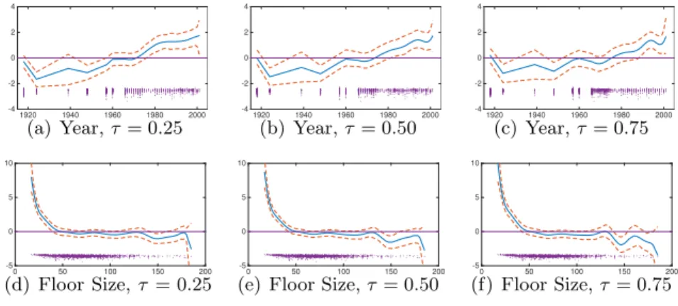
Figures2.6and2.7show the estimated non-linear effect for the year of con-struction and the floor size using Gaussian and Lasso priors respectively. The points below each sub-figure represent the available observations for each value of the covariates, while dotted lines represent the 95% posterior credible intervals. We can observe that both priors provide similar esti-mated splines for the effect of floor size on house prices. Small flats (less that 40m2) have a very high rent per square meter, while for big flats the rent remains almost unchanged. For the year of construction, the estimated splines are relatively different under the two prior specifications but they actually contain similar information. When looking at the level and confi-dence intervals of the variable, the effect of this covariate is almost null until the 1990s, when a clear positive and increasing effect is shown under both

(38)

1920 1940 1960 1980 2000 -4 -2 0 2 4 (a) Year,τ = 0.25 1920 1940 1960 1980 2000 -4 -2 0 2 4 (b) Year,τ= 0.50 1920 1940 1960 1980 2000 -4 -2 0 2 4 (c) Year,τ = 0.75 0 50 100 150 200 -5 0 5 10 (d) Floor Size, τ = 0.25 0 50 100 150 200 -5 0 5 10

(e) Floor Size,τ= 0.50

0 50 100 150 200 -5 0 5 10 (f) Floor Size,τ = 0.75

Figure 2.6: Estimated non-parametric effect using Gaussian prior with 95% credible bands for Munich data.

prior specifications. Figure 2.8displays the estimated spatial effects of 380 subquarters in Munich. Values are normalized to be in the range (0,1). As expected, for both Gaussian and Lasso priors, rents are high in the centre of Munich and some well–known districts, becoming lower on the margins. Finally, estimated posterior means and standard deviations for the linear parametric effects are shown in Table 2.5. The signs of the variables are in line with previous work; however, under Lasso prior some new findings are associated with the effect of the following variables: No hot water, No central heating and 6 Rooms. Interestingly, Lasso prior differentiate the effect of these variables for each quantile. We find that the absence of hot water and the presence of 6 Rooms have a statistically significant negative effect only on expensive houses, i.e. forτ = 0.75 while the opposite occurs for the absence of central heating. We argue that these results highlight the variety of the consumption choices due to different budget constraints.It is worth noting that Lasso prior correctly shrinks the effect of Special bath-room interior, that is not very significant when estimated using Gaussian prior.

2.6.3 Barro growth data

Our final application, is an analysis of the dataset underlying the interna-tional economic growth model, firstly considered by Barro and Sala i-Martin (1995) and extended to the quantile regression framework by Koenker and