Essays on economic forecasting using machine learning

Lauri Nevasa lmi E 6 7 UNIVERSIT ATIS TURKUENSIS ISBN 978-951-29-8222-6 (PRINT) ISBN 978-951-29-8223-3 (PDF) Painosalama Oy , T urku, F inland 2 02 0 –

ESSAYS ON ECONOMIC

FORECASTING USING

MACHINE LEARNING

Lauri Nevasalmi

–

~~

OFTURKU

ESSAYS ON ECONOMIC

FORECASTING USING

MACHINE LEARNING

Lauri Nevasalmi

Turku School of Economics Department of Economics Economics

Doctoral programme of Turku School of Economics

Supervised by

Professor Heikki Kauppi University of Turku Turku, Finland

Professor Matti Viren University of Turku Turku, Finland

Reviewed by

Professor Charlotte Christiansen Aarhus University

Aarhus, Denmark

Professor Seppo Pynnönen University of Vaasa

Vaasa, Finland

Opponent

Professor Charlotte Christiansen Aarhus University

Aarhus, Denmark

The originality of this publication has been checked in accordance with the University of Turku quality assurance system using the Turnitin OriginalityCheck service.

ISBN 978-951-29-8222-6 (PRINT) ISBN 978-951-29-8223-3 (PDF) ISSN 2343-3159 (Painettu/Print)

ISSN 2343-3167 (Verkkojulkaisu/Online) Painosalama, Turku, Finland 2020

Department of Economics Economics

LAURI NEVASALMI: Essays on economic forecasting using machine learning

Doctoral Dissertation, 163 pp.

Doctoral Programme of Turku School of Economics November 2020

ABSTRACT

This thesis studies the additional value introduced by different machine learning methods to economic forecasting. Flexible machine learning methods can discover various complex relationships in data and are well-suited for analysing so called big data and potential problems therein. Several new extensions to existing machine learning methods are proposed from the viewpoint of economic forecasting.

In Chapter 2, the main objective is to predict U.S. economic recession periods with a high-dimensional dataset. A cost-sensitive extension to the gradient boosting machine learning algorithm is proposed, which takes into account the scarcity of recession periods. The results show how the cost-sensitive extension outperforms the traditional gradient boosting model and leads to more accurate recession forecasts.

Chapter 3 considers a variety of different machine learning methods when predicting daily returns of the S&P 500 stock market index. A new multinomial approach is suggested, which allows us to focus on predicting the large absolute returns instead of the noisy variation around zero return. In terms of both the statistical and economic evaluation criteria gradient boosting turns out to be the best-performing machine learning method.

In Chapter 4, the asset allocation decisions between risky and risk-free assets are determined using a flexible utility maximization based approach. Instead of the merely considered two-step approach where portfolio weights are based on the excess return predictions obtained with statistical predictive regressions, here the optimal weights are found directly by incorporating a custom objective function to the gradient boosting algorithm. The empirical results using monthly U.S. market returns show that the utility-based approach leads to substantial and quantitatively meaningful economic value over the past approaches.

Turun Kauppakorkeakoulu Taloustieteen laitos

Taloustiede

LAURI NEVASALMI: Essays on economic forecasting using machine learning

Väitöskirja, 163 s.

Turun Kauppakorkeakoulun Tohtoriohjelma Marraskuu 2020

TIIVISTELMÄ

Tässä väitöskirjassa tarkastellaan millaista lisäarvoa koneoppimismenetelmät voivat tuoda taloudellisiin ennustesovelluksiin. Joustavat koneoppimismenetelmät kyke-nevät mallintamaan monimutkaisia funktiomuotoja ja soveltuvat hyvin big datan eli suurten aineistojen analysointiin. Väitöskirjassa laajennetaan koneoppimismene-telmiä erityisesti taloudellisten ennustesovellusten lähtökohdista katsoen.

Luvussa 2 ennustetaan Yhdysvaltojen talouden taantumajaksoja käyttäen hyvin suurta selittäjäjoukkoa. Gradient boosting -koneoppimismenetelmää laajennetaan huomioimaan aineiston merkittävä tunnuspiirre eli se, että taantumajaksoja esiintyy melko harvoin talouden ollessa suurimman osan ajasta noususuhdanteessa. Tulokset osoittavat, että laajennettu gradient boosting -menetelmä kykenee ennustamaan tulevia taantumakuukausia huomattavasti perinteisiä menetelmiä tarkemmin.

Luvussa 3 hyödynnetään useampaa erilaista koneoppimismenetelmää S&P 500 -osakemarkkinaindeksin päivätuottojen ennustamisessa. Aiemmista lähestymis-tavoista poiketen tässä tutkimuksessa kategorisoidaan tuotot kolmeen eri luokkaan pyrkimyksenä keskittyä informatiivisempien suurten positiivisten ja negatiivisten tuottojen ennustamiseen. Tulosten perusteella gradient boosting osoittautuu parhaaksi menetelmäksi niin tilastollisten kuin taloudellistenkin ennustekriteerien mukaan.

Luvussa 4 tarkastellaan, kuinka perinteisen tuottoennusteisiin nojautuvan kaksi-vaiheisen lähestymistavan sijaan allokaatiopäätös riskisen ja riskittömän sijoitus-kohteen välillä voidaan muodostaa suoraan sijoittajan kokeman hyödyn pohjalta. Hyödyn maksimoinnissa käytetään gradient boosting -menetelmää ja sen mahdol-listamaa itsemäärättyä tavoitefunktiota. Yhdysvaltojen aineistoon perustuvat empii-riset tulokset osoittavat kuinka sijoittajan hyötyyn pohjautuva salkkuallokaatio johtaa perinteistä kaksivaiheista lähestymistapaa tuottavampiin allokaatiopäätöksiin.

After completing my Master’s Thesis the idea of learning more about binary dependent variable models grew inside me. In Finland there are only a few people with an in-depth knowledge on this matter. Soon after starting my career as a doctoral student I found myself working with both of them.

First of all, I would like to thank my thesis supervisor Professor Heikki Kauppi. Thank you for introducing me to the Turku School of Economics and providing me the chance to pursue my goals. Also thank you for the endless amount of fexibility when it comes to meeting arrangements or adapting to new situations in life. We have had many extremely fruitful discussions from which I have learned so much. Who would have thought that your vague idea to give a closer look at one particular paper on machine learning resulted in an entire Doctoral Thesis and an additional Master’s degree on the matter?

Next my deepest gratitude goes towards Associate Professor Henri Nyberg. You have always found the time to carefully read and comment my ongoing work. Without your help throughout the years I would not be writing this. Also thank you for constantly challenging me as a young scientist. Whether it was about frst public appearance or frst submission you always pushed me forward but also provided invaluable help when needed. I am extremely grateful for all the things you have done for me. I can not thank you enough so I sincerely hope the color of Manchester will be red in the near future.

Thank you Susanne and Salla for getting the best out of the hectic frst year as a doctoral student. The unforgettable year provided many great memories and hopefully life-long friendships. I wish to thank the pre-examiners of my thesis, Professor Charlotte Christiansen and Professor Seppo Pynnönen, for their insightful comments and suggestions. The long list of people who have given helpful comments on different parts of this thesis receive my utmost appreciation at the beginning of each corresponding chapter. The fnancial support from the Emil Aaltonen foundation (personal grant and project funding) and the Academy of Finland (grant 321968) is also gratefully acknowledged. Similarly, I am greatly indebted to my parents for the help

Finally, I would like to thank my wife Mari. Thank you for always believing in me and being there for me when things seemed helpless. I am forever grateful for being able to reach towards my dreams knowing that our children are having the best of times with you. And no matter what life brings ahead of us after graduation, I could not feel more confdent as long as I am with you. Thank you Leevi, Milli and Masi for reminding me how the little things in life matter and always putting a smile on my face. This thesis is dedicated to all of you.

Espoo, October 2020 Lauri Nevasalmi

Abstract iii

Tiivistelmä iv

1 Introduction 1

1.1 Background . . . 1

1.2 Econometric framework . . . 3

1.2.1 More fexible functional forms using machine learning 4 1.2.2 Loss function . . . 7

1.3 Summary of the essays . . . 8

1.3.1 Recession forecasting with big data . . . 9

1.3.2 Forecasting multinomial stock returns using machine learning methods . . . 9

1.3.3 Moving forward from predictive regressions: Boosting asset allocation decisions . . . 10

References . . . 11

2 Recession forecasting with big data 15 2.1 Introduction . . . 16

2.2 Methodology . . . 19

2.2.1 Gradient boosting . . . 19

2.2.2 Cost-sensitive gradient boosting with class weights . . 22

2.2.3 Regularization parameters in gradient boosting . . . . 25

2.3 Results . . . 27

2.3.1 Data and model setup . . . 27

2.3.2 In-sample results . . . 29

2.3.3 Out-of-sample results . . . 33

2.4 Conclusions . . . 37

ods 43

3.1 Introduction . . . 44

3.2 Methodology . . . 46

3.2.1 Multinomial stock returns . . . 46

3.2.2 Machine learning methods . . . 49

3.3 Data and model setup . . . 61

3.3.1 Data . . . 61

3.3.2 Tuning parameter optimization . . . 65

3.4 Empirical results . . . 67

3.4.1 Statistical predictive performance . . . 67

3.4.2 Economic predictive performance . . . 70

3.5 Conclusions . . . 75

References . . . 77

Appendix A: Full predictor set . . . 81

Appendix B: Model selection results of the tree-based methods . . . 83

4 Moving forward from predictive regressions: Boosting asset allo-cation decisions 85 4.1 Introduction . . . 86

4.2 Methodology . . . 89

4.2.1 Starting point and two-step statistical approach . . . . 89

4.2.2 Objective function . . . 94

4.2.3 Customized gradient boosting . . . 97

4.3 Empirical results . . . 101

4.3.1 Dataset . . . 101

4.3.2 Evaluation and benchmarks . . . 103

4.3.3 In-sample (full sample) results . . . 106

4.3.4 In-sample extensions . . . 111

4.3.5 Out-of-sample forecasting results . . . 113

4.4 Discussion . . . 117

4.5 Conclusions . . . 120

References . . . 121

Tables and Figures . . . 125

Introduction

1.1 Background

The amount of data has grown exponentially in the previous decade. The ever-increasing fow of information opens up a wide range of completely new possibilities for economic research. Various studies show how web searches or satellite images, for example, can be used to predict economic activity (see e.g., Ettredge, Gerdes and Karuga, 2005; Choi and Varian, 2012; Henderson, Storeygard and Weil, 2012). New data-related issues such as missing data, large amount of potential predictors and mixed data types arise with such ’modern’ economic data. Mullainathan and Spiess (2017) emphasize how the term big data refects the change in both the scale and nature of data. The demand for fexible methods that can handle such datasets and the potential problems therein grows rapidly both in the industry as well as academia.

The popularity of fexible machine learning methods has been increasing in the previous two decades. Machine learning methods are typically introduced to economic forecasting as a tool to exploit the potential non-linearities in the dataset (see e.g., Stock and Watson, 1999; Kuan and Liu, 1995). Other interest-ing features of machine learninterest-ing, such as the model selection capabilities of certain methods, have received attention only recently (see e.g., Bühlmann, 2006; Wohlrabe and Buchen, 2014). This thesis puts emphasis on both ap-proaches and studies the additional value introduced by different machine learning methods to economic forecasting. Not just by allowing for more fexible functional forms in the data but also in terms of the ability to deal

with various issues that can be encoutered in economic forecasting problems with big data. These include studying the class imbalance problem with a high-dimensional dataset or even customizing the entire objective function to better meet the needs of a particular forecasting problem.

The class imbalance and the effects on classifcation is well covered in the machine learning literature (see e.g., Galar et al., 2012). Suprisingly the class imbalance problem has not been properly taken into consideration in previous economic research. That is the case despite the numerous potential economic applications, such as recession forecasting or fraud detection, where the binary response can be quite severely imbalanced. Moreover, most of the standard machine learning algorithms assume balanced class distributions and hence the forecasting performance can be deteriorated in the presence of class imbalance (see He and Garcia, 2009). On the other hand, customizing the entire objective function is connected to the recent discussion by Elliott and Timmermann (2016, Chapter 2) on what is the appropriate objective function in econometric inference. In this thesis we introduce an innovative synthesis between fnancial economics and machine learning. This is done by utilizing the gradient boosting machine learning algorithm as a tool to optimize a custom objective function motivated by economics and fnance.

In an ideal situation the economic forecasting model is based on economic theory and the main analysis concerns specifying the exact functional form for the relationship between the dependent variable and the predictors. Majority of the time however the fnal model composition (and the functional form) is purely empirical. But how to identify the optimal predictor set? Several potential predictor candidates have been discovered in the economic literature starting from the pioneering work of Mitchell and Burns (1938). Different fnancial variables have shown predictive power beyond the benchmark au-toregressive specifcations when forecasting GDP growth, whereas the yield curve is the single best predictor of economic recession periods for example (see e.g., Stock and Watson, 2003; Wheelock and Wohar, 2009). In such a data-rich environment induced by the recent growth in the availability and accessibility of data the amount of potential predictive variables can be very large (see e.g., Bühlmann, 2006). Traditional econometric methods can only handle very limited predictor sets at a time and some sort of model selection procedure is required. Such procedure can easily become computationally

very demanding or even infeasible as the number of predictors grow.

The ability to handle large predictor sets also varies between different ma-chine learning methods. The risk of overlearning the data with large predictor sets is a serious issue for many commonly used machine learning methods. Methods such as the support vector machines or nearest neighbor are known to suffer from the curse of dimensionality (see e.g., Hastie, Tibshirani and Friedman, 2009). Ensemble methods random forest and gradient boosting machine on the other hand contain an attractive feature as model selection is conducted simultaneously with model estimation. These methods require no prior knowledge on the relevance of different predictors and can provide important details about the most informative predictive variables. For a more detailed description of the internal variable selection associated with these two methods, see Breiman (2001) and Friedman (2001).

Unlike in various business-oriented applications the computational eff-ciency of the forecasting method does not play a signifcant role as the amount of observations in economic datasets is typically quite limited. Economic fore-casting however places a different type of restriction on the selected method. Although accurate fnal predictions possibly exploiting non-linearities in the data is the ultimate goal, the econometrician favours interpretable models (Einav and Levin, 2014). Some machine learning methods, such as neural networks, fall in the category of so called ’black-box’ models (Hastie et al., 2009). Such models provide no exact information on the linkages between the response and the predictive variables or this information is hard to visualize. Thus the interpretability of the model, in addition to the ability to handle potentially large predictor sets, needs to be taken into account when selecting the appropriate forecasting method with modern economic data.

The rest of this introductory chapter is organized as follows. Section 1.2 presents the econometric framework with different machine learning methods by allowing for various functional forms and loss functions. In addition, short summaries of the three essays are presented in Section 1.3.

1.2 Econometric framework

This section considers the underlying functional forms and objective functions of the fve machine learning methods used in this thesis. These are the gradient

boosting machine, random forest, neural networks, support vector machine and k-nearest neighbor method.

1.2.1 More fexible functional forms using machine learning

The goal of statistical modelling and prediction is to specify the functional relationship between the dependent variable and the predictors. In economic forecasting we typically assume the response at time t+h, where h is the forecast horizon, to be a function of the predictive variables and forecast error yt+h =F(xt) +et+h, t= 1,...,N, (1.1)

where yt+h is the response, F(xt)is a potentially non-linear function of the

predictors xt and et+h is the forecast error. In order to make the function

approximation strategy feasible F(·)is typically restricted to certain parame-terized class of functions.

Linear regression model has been the cornerstone of statistical analysis for several decades (Hastie et al., 2009). In the linear regression model we assume the underlying functional form to be a linear function of the predictor variables

0

F(xt) =β0 +xtβ, (1.2)

where β0is the constant term and xtis a p×1vector of predictors. For many

real-world applications the assumption of linearity is very restrictive. Machine learning methods allow for more fexible functional forms and can discover all sorts of complex relationships in data. It should however be noted that the linearity assumption could easily be incorporated to majority of these methods as well.

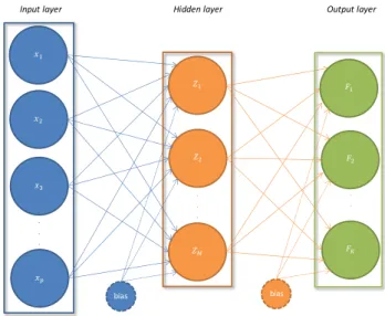
As an extension to the linear model in (1.2) let us consider a single hidden-layer feed-forward neural network with linear output. In this case the network consists of three layers: the input layer, a single hidden layer with M hidden nodes and the output layer. The subsequent layers in the network are con-nected with each other through weights. The network architecture induced by the assumptions of a single hidden-layer and feed-forward weights is the most commonly used one in practice (Bishop, 2006). The fnal model in such a network is a linear combination of the original predictors going through a

non-linear activation function

M

X ₀

F(xt) = γmσ(bm+xtαm), (1.3) m=1

where bm is a bias term and αmis a p×1vector of weights connecting the

predictors to the hidden node m. Similarly γmis the weight connecting the

hidden node mto the fnal output node. One can note the resemblance of the term inside the brackets to the linear model provided in (1.2). Without the non-linear activation function σ(·), which usually is a sigmoid function or hyperbolic tangent, the fnal output would be a linear combination of linear combinations and hence also linear. The total amount of hidden nodes M limits the range of functions that a single hidden layer neural network model can approximate. With a suffcient amount for Mthe model in (1.3) can approximate any continuous function to arbitrary accuracy (see e.g., Hornik, Stinchcombe and White, 1989; Cybenko, 1989).

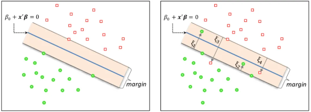
In the support vector machine by Vapnik (1995) non-linearity is intro-duced to the model by transforming the original input feature space into an enlarged space using non-linear functions. In a classifcation context the data could be linearly separable in this higher dimensional feature space. By considering a d-dimensional set of transformation functions we have h(xt) = (h1(xt), . . . , hd(xt))0and the fnal model can be written as

F(xt) =β0+h(xt)0β. (1.4)

Note that although the classifcation problem might be linearly separable in the higher dimensional feature space, when transformed back to the original feature space it results in a non-linear decision boundary. Instead of the exact transformation h(xt) a kernel function, which computes inner products in

the transformed space, is suffcient. A radial basis function and a dth-degree polynomial are typical choices for the kernel function (Hastie et al., 2009). With a linear kernel the fnal output is also a linear function of the predictors. Linear regression model in (1.2) assumes a global linear function whereas in the k-nearest neighbor method originally presented by Fix and Hodges (1951) the underlying function is assumed to be well approximated by a locally constant function. Let κ(xt)denote the indices of the kobservations closest to

xtbased on some distance metric. With a continuous response the fnal model

in k-nearest neighbor method is simply an average of the kresponses

X

1

F(xt) = yi+h, (1.5)

k

i∈κ(xt)

where yi+h is the response attached to index i(taking into account the

fore-casting horizon h). In the classifcation approach the fnal model is based on a majority vote between the kdatapoints and ties are broken at random. Parameter kcontrols for the complexity of the model, where smaller values for kresult in more fexible models (Bishop, 2006).

In the ensemble methods random forest and gradient boosting the fnal model, also called an ensemble, has an additive form

M X

F(xt) = fm(xt), (1.6)

m=1

where fm(xt)is the base learner function at iteration m. Note that the single

hidden-layer feed-forward network in (1.3) and the support vector machine in (1.4) can also be seen as additive models with unique base learner functions (Friedman, 2001). In random forest the base learner in (1.6) is a classifcation or regression tree, while in gradient boosting one can consider for example linear or spline based functions as well.

The power of random forest is based on creating a collection of inde-pendent trees that are minimally correlated with each other (Breiman, 2001). Depending on the learning problem the fnal prediction is either a majority vote or an average of the predictions induced by each individual tree. Gra-dient boosting takes a slightly different approach as the fnal model is built in a forward stagewise manner by adding new base learner functions to the ensemble that best ft the negative gradient of the loss function. Provided with suffcient amount of data and a fexible base learner, such as regression trees or smoothing splines, boosting can basically approximate any kind of functional form.

1.2.2 Loss function

In the general estimation problem the goal is to fnd the function F(xt)that

minimizes the expected loss of some predefned loss function

b

F(xt)=argminE[L(yt+h, F(xt))], (1.7) F(xt)

where yt+h is the response and xtis a vector of predictor variables. As was

considered in the previous section the optimal function with each method is assumed to belong to some predefned class of functions. The actual functional form of the loss function L(·)in (1.7) depends on both the response and the considered machine learning method. In economic forecasting problems the response is typically either continuous or discrete with two or more classes.

With a continuous response both the traditional linear regression model and majority of the machine learning methods aim to minimize the (sample) sum of squared error (SSE)

N

X � 2

LSSE = yt+h−F(xt) . (1.8)

t=1

In the binary two-class classifcation problem the typically considered loss function is the binomial deviance. Using more familiar terminology the bino-mial deviance can simply be expressed as the negative log-likelihood (Hastie et al., 2009). Assuming a logistic transformation function the deviance can be written as

N

X �

LDev=− yt+hF(xt)−log(1+exp(F(xt))) . (1.9) t=1

In the multinomial extension there are L classes and a separate functional estimate Fl(xt)for each class. By denoting each class lof the multinomial

response with a separate binary variable yt+h,lthe multinomial deviance can

be written as

N L

X X

LMDev =− yt+h,l log(pt,l(xt)), (1.10) t=1 l=1

The support vector machine takes a slightly different approach. The orig-inal idea of support vector machine is presented in a classifcation context, where the fnal goal is to produce a margin maximizing classifer (see Vapnik, 1995). Evgeniou, Pontil and Poggio (2000) however show that the optimiza-tion problem in support vector machine can also be presented in terms of minimizing a regularized loss function

N X

LSVM = V(yt+h, F(xt))+λJ(F). (1.11) t=1

In support vector machines we have a specifc form for both the general error measure V(·)and the penalty function J(·). The general error measure also depends on whether we are dealing with a regression or classifcation problem.

Random forest and k-nearest neighbor algorithm can not be conceived as direct optimization procedures. The k-nearest neighbor algorithm by Fix and Hodges (1951) is a model-free method since the classifcation or prediction of a new observation is based purely on the data points of the training set. The search for the k nearest neighbors to each new datapoint is based on some distance measure say the euclidean distance, but this distance metric can not be considered as a conventional loss function. Similarly for random forest although each independent tree in the fnal ensemble is optimized based on the usual criterions with classifcation and regression trees, such as the least squares criterion or the gini index, the entire ensemble is not directly optimizing any loss function (Wyner et al., 2017).

1.3 Summary of the essays

In this section, we review three empirical applications on economic forecasting using machine learning methods. In Section 1.3.1, we study the predictability of binary economic recession periods. Section 1.3.2 considers predicting multi-nomial stock returns, where the continuous daily stock returns are discretized into three classes. In the last section we take a step further from the classical stock return predictability studies and focus on optimizing asset allocation decisions directly.

1.3.1 Recession forecasting with big data

In this chapter we study the ability of the gradient boosting machine to fore-cast economic recession periods in the U.S. using high-dimensional data. Recessions are shorter events compared to expansion periods leading to quite heavily imbalanced binary class labels. The class imbalance with large amount of predictive variables creates a risk of forecasting only the non-recessionary periods well. We propose a new cost-sensitive extension to the gradient boost-ing model usboost-ing binary class weights. In this approach the sample counterpart of (1.7) is a weighted average instead of the arithmetic mean. We use the data-based approach by Zhou (2012) and choose the binary weights according to the class imbalance observed in the dataset. To the best of our knowledge cost-sensitive gradient boosting model using class weights has not been utilized in previous economic research.

The results confrm the fnding of Blagus and Lusa (2017) who note that the performance of a gradient boosting model can be rather poor with high class imbalance, especially when a high-dimensional dataset is used. The cost-sensitive extension to the gradient boosting model using class weights can take the class imbalance problem into account and produces strong warning signals for the U.S. recessions with different forecasting horizons. Different types of interest rate spreads are the most important predictors with each forecasting horizon.

1.3.2 Forecasting multinomial stock returns using machine learn-ing methods

The fve different machine learning methods presented in Section 1.2 are compared in their ability to predict the daily returns of the S&P 500 stock market index. Majority of the previous research focus on predicting the actual level and then partly the direction of stock returns (i.e. the signs of stock returns, indicating that we are interested in a binary-dependent time series generated from returns). In this chapter the returns are categorized into three classes based on the upper and lower quartiles of the return series. The less informative and noisy fuctuation associated with small absolute returns is isolated in one class and the other two focus on predicting the large absolute returns. To the best of our knowledge such multinomial approach has not

been taken into consideration in previous economic research.

All the machine learning methods examined produce multinomial classi-fcation results which are signifcant from both the statistical and economic point of view. Among the machine learning methods considered the gradient boosting machine turns out to be the top-performer. The results also show how the predictability of large absolute returns tend to cluster around certain periods of time. These periods are typically associated with high stock market volatility. The conclusion of increased predictability during market turmoil is in line with the fndings of Krauss, Do and Huck (2017) and Fiévet and Sornette (2018).

1.3.3 Moving forward from predictive regressions: Boosting asset allocation decisions

As pointed by Leitch and Tanner (1991), among many others, the statistically signifcant predictability of stock returns does not necessarily imply economic proftability and vice versa. For an individual investor or portfolio manager the economic value of the predictions is the ultimate goal instead of the merely considered statistical predictability. In this chapter we estimate the portfolio weights directly using gradient boosting by incorporating a custom objective function in the context of (1.7). Our contribution is strongly connected to a more general issue in (fnancial) econometrics on what is the appropriate objec-tive (loss) function in econometric inference (see e.g., Elliott and Timmermann, 2016, chapter 2).

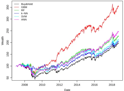
Our empirical results on the monthly U.S. market returns show that sub-stantial and quantitatively meaningful economic value can be obtained with our utility boosting method. Technical indicators yield as a group the largest benefts in out-of-sample forecasting experiments. This is generally in line with the conclusions of Neely et al. (2014) and now confrmed with very different methodology.

References

Bishop, C. M. (2006). Pattern Recognition and Machine Learning (Information Science and Statistics). Springer-Verlag, Berlin, Heidelberg.

Blagus, R. and Lusa, L. (2017). Gradient boosting for high-dimensional pre-diction of rare events. Computational Statistics & Data Analysis, 113:19 – 37.

Breiman, L. (2001). Random forests. Machine Learning, 45(1):5–32.

Bühlmann, P. (2006). Boosting for high-dimensional linear models. Annals of Statistics, 34(2):559–583.

Choi, H. and Varian, H. (2012). Predicting the present with google trends.

Economic Record, 88(s1):2–9.

Cybenko, G. (1989). Approximation by superpositions of a sigmoidal function.

Mathematics of Control, Signals, and Systems, 2(4):303–314.

Einav, L. and Levin, J. (2014). Economics in the age of big data. Science, 346(6210).

Elliott, G. and Timmermann, A. (2016). Economic Forecasting. Princeton Uni-versity Press, 1 edition.

Ettredge, M., Gerdes, J., and Karuga, G. (2005). Using web-based search data to predict macroeconomic statistics. Commun. ACM, 48(11):87–92.

Evgeniou, T., Pontil, M., and Poggio, T. A. (2000). Regularization networks and support vector machines. Advances in Computational Mathematics, 13:1–50. Fiévet, L. and Sornette, D. (2018). Decision trees unearth return sign

pre-dictability in the s&p 500. Quantitative Finance, pages 1–18.

Fix, E. and Hodges, J. (1951). Discriminatory Analysis: Nonparametric Discrimi-nation: Consistency Properties. USAF School of Aviation Medicine, Randolph Field, TX.

Friedman, J. H. (2001). Greedy function approximation: A gradient boosting machine. Annals of Statistics, 29(5):1189–1232.

Galar, M., Fernández, A., Tartas, E. B., Bustince, H., and Herrera, F. (2012). A review on ensembles for the class imbalance problem: Bagging-, boosting-, and hybrid-based approaches. IEEE Transactions on Systems, Man, and Cyber-netics, Part C (Applications and Reviews), 42:463–484.

Hastie, T., Tibshirani, R., and Friedman, J. (2009). The elements of statistical learning: data mining, inference and prediction. Springer, 2 edition.

He, H. and Garcia, E. A. (2009). Learning from imbalanced data. IEEE Transactions on Knowledge and Data Engineering, 21(9):1263–1284.

Henderson, J. V., Storeygard, A., and Weil, D. N. (2012). Measuring economic growth from outer space. American Economic Review, 102(2):994–1028. Hornik, K., Stinchcombe, M., and White, H. (1989). Multilayer feedforward

networks are universal approximators. Neural Networks, 2(5):359 – 366. Krauss, C., Do, X. A., and Huck, N. (2017). Deep neural networks,

gradient-boosted trees, random forests: Statistical arbitrage on the s&p 500. European Journal of Operational Research, 259(2):689 – 702.

Kuan, C.-M. and Liu, T. (1995). Forecasting exchange rates using feedforward and recurrent neural networks. Journal of Applied Econometrics, 10(4):347–364. Leitch, G. and Tanner, J. E. (1991). Economic forecast evaluation: Profts

versus the conventional error measures. The American Economic Review, 81(3):580–590.

Mitchell, W. C. and Burns, A. F. (1938). Statistical Indicators of Cyclical Revivals. NBER.

Mullainathan, S. and Spiess, J. (2017). Machine learning: An applied econo-metric approach. Journal of Economic Perspectives, 31(2):87–106.

Neely, C. J., Rapach, D. E., Tu, J., and Zhou, G. (2014). Forecasting the eq-uity risk premium: The role of technical indicators. Management Science, 60(7):1772–1791.

Stock, J. H. and Watson, M. W. (1999). A Comparison of Linear and Nonlinear Uni-variate Models for Forecasting Macroeconomic Time Series, pages 1–44. Oxford University Press, Oxford.

Stock, J. H. and Watson, M. W. (2003). Forecasting output and infation: The role of asset prices. Journal of Economic Literature, 41(3):788–829.

Vapnik, V. N. (1995). The Nature of Statistical Learning Theory. Springer-Verlag, Berlin, Heidelberg.

Wheelock, D. C. and Wohar, M. E. (2009). Can the term spread predict output growth and recessions? a survey of the literature. Federal Reserve Bank of St. Louis Review, 91:419–440.

Wohlrabe, K. and Buchen, T. (2014). Assessing the macroeconomic forecasting performance of boosting: Evidence for the united states, the euro area and germany. Journal of Forecasting, 33(4):231–242.

Wyner, A. J., Olson, M., Bleich, J., and Mease, D. (2017). Explaining the success of adaboost and random forests as interpolating classifers. Journal of Machine Learning Research, 18(48):1–33.

Zhou, Z.-H. (2012). Ensemble Methods: Foundations and Algorithms. Chapman & Hall/CRC, 1st edition.

Recession forecasting with big

data

Abstract ∗ †

In this chapter, a large amount of different fnancial and macroeconomic variables are used to predict the U.S. recession periods. We propose a new cost-sensitive extension to the gradient boosting model which can take into account the class imbalance problem of the binary response variable. The class imbalance, caused by the scarcity of recession periods in our application, is a problem that is emphasized with high-dimensional datasets. Our empirical results show that the introduced cost-sensitive extension outperforms the traditional gradient boosting model in both in-sample and out-of-sample forecasting. Among the large set of candidate predictors, different types of interest rate spreads turn out to be the most important predictors when forecasting U.S. recession periods.

∗

The author would like to thank Heikki Kauppi, Henri Nyberg, Simone Maxand and seminar participants at the Annual Meeting of the Finnish Economic Association and FDPE Econometrics workshop for constructive comments. The fnancial support from the Emil Aaltonen Foundation is gratefully acknowledged.

†

2.1 Introduction

Recessions are painful periods with a signifcant and widespread decline in economic activity. Early warning signals of recessions would be important for different kinds of economic agents. Households, frms, policymakers and central bankers could all utilize the information concerning upcoming economic activity in their decision making. The probability of a recession is fairly straightforward to interpret and can be easily taken into consideration in all kinds of economic decision making.

But what are the indicators that consistently lead recessions? Since the early work of Estrella and Mishkin (1998) there has been a large amount of empirical research concerning the predictive content of different economic and fnancial variables (see e.g., Nyberg, 2010; Liu and Moench, 2016). The amount of potential recession indicators is growing rapidly as the constraints related to data-availability and computational power keep diminishing. Traditionally used binary logit and probit models can only handle small predictor sets at a time, which makes the search for the best predictors quite diffcult.

Recent developments in the machine learning literature provide a solution to this problem. State of the art supervised learning algorithm called gradient boosting is able to do variable selection and model estimation simultaneously. Non-parametric boosting can handle huge predictor sets and the estimated conditional probability function can take basically any kind of form. The main objective of this research is to explore how we can exploit high-dimensional datasets when making recession forecasts with the gradient boosting model.

The business cycle consists of positive and negative fuctuations around the long-run growth rate of the economy. These fuctuations are also known as expansions and recessions. The offcial business cycle chronology for the U.S. is published by the National Bureau of Economic Research (NBER). Recessions are shorter events compared to expansion periods leading to quite heavily imbalanced binary class labels. In our dataset less than 14 percent of the monthly observations are classifed as recessions. This class imbalance and the effects on classifcation is well covered in the machine learning literature (see e.g., Galar et al., 2012). Suprisingly the scarcity of recession periods has not been properly taken into consideration in previous economic research.

classes: resampling techniques and cost-sensitive learning methods (see e.g., He and Garcia, 2009). Resampling is the easiest and most commonly used alternative. The dataset could be balanced by drawing a random sample without replacement from the majority class, which is called undersampling. In the recession forecasting setup the size of the dataset is already very limited so this could create problems when estimating the model, especially with high-dimensional data. In the oversampling approach the idea is to sample with replacement from the minority class. He and Garcia (2009) argue that the duplicate observations from the minority class can lead to overftting.

Instead of replicating existing observations from the minority class one could learn the characteristics in this class and create synthetic samples based on feature space similarities. This synthetic minority oversampling technique also known as SMOTE is a popular alternative when dealing with imbalanced data. Blagus and Lusa (2013) however fnd that variable selection is needed before running SMOTE on high-dimensional datasets.

Cost-sensitive learning methods can take the class imbalance into account without artifcially manipulating the dataset. In a variety of real-life classifca-tion problems, such as recession forecasting or fraud detecclassifca-tion, misclassifying the minority class can be considered very costly. The cost-sensitivity can be incorporated into the model by attaching a higher penalty for misclassifying the minority class. Several modifed versions of the adaboost algorithm by Freund and Schapire (1996) exist, where the weight updating rule of the origi-nal algorithm is modifed to better account for the class imbalance (see e.g., Sun et al., 2007; Fan et al., 1999; Ting, 2000).

This is natural since weight updating is a crucial part of the adaboost algorithm designed purely for classifcation problems. However this is not the case with the more general gradient boosting algorithm presented by Friedman (2001) that can handle variety of problems beyond classifcation and the sensitivity have to be incorporated otherwise. We propose a cost-sensitive extension to the gradient boosting model by introducing a binary class weight to each observation in the dataset that refect the asymmetric misclassifcation costs. To the best of our knowledge cost-sensitive gradient boosting model using class weights has not been utilized in previous economic research.

economic research with mixed results. Ng (2014) uses the gradient boosting model with stump regression trees to predict recession periods in the U.S. The dataset used by Ng (2014) has a fairly large predictor set and is from the same source as the dataset used in this paper. With this model setup Ng (2014) concludes that the gradient boosting model is far from perfect in forecasting recessions.

Berge (2015) uses a smaller predictor set to forecast U.S. recessions with the gradient boosting model. The results show how boosting outperforms other model selection techniques such as Bayesian model averaging. Moreover, the results highlight the importance of non-linearity in recession forecasting as boosting with non-linear smoothing splines outperforms boosting with a linear fnal model. Döpke, Fritsche and Pierdzioch (2017) succesfully forecast German recession periods with the gradient boosting model using regression trees. Unlike Ng (2014) they build larger trees which allow for potential interaction terms between predictors. This approach is used in this study as well.

Our results confrm the fnding of Blagus and Lusa (2017) who note that the performance of a gradient boosting model can be rather poor with high class imbalance, especially when a high-dimensional dataset is used. The out-of-sample forecasting ability of the traditional gradient boosting model is quite heavily deteriorated compared to the in-sample results. The cost-sensitive extension to the gradient boosting model using class weights can take the class imbalance problem into account and produces strong warning signals for the U.S. recessions with different forecasting horizons.

The cost-sensitive gradient boosting models estimated using huge pre-dictor sets rely heavily on different kinds of interest rate spreads. This is also the case with the short and medium term forecasting horizons although different variables related to the real economy are also available in the dataset. The internal model selection capability of gradient boosting confrms that predictors with predictive power beyond the term spread are quite hard to fnd (see e.g., Estrella and Mishkin, 1998; Liu and Moench, 2016).

The results also show how the chosen lag length for a predictor can vary substantially from the forecasting horizon considered. A similar observation has been made by Kauppi and Saikkonen (2008) in the conventional probit model. The term spread is the dominant predictor when forecasting recessions

one year ahead, which is a common fnding in the previous literature (see e.g., Dueker, 1997; Estrella and Mishkin, 1998).

The rest of the paper is organized as follows. The gradient boosting framework and the cost-sensitive extension to the gradient boosting model are introduced in Section 2.2. The dataset and the empirical analysis are presented in Section 2.3. Section 2.4 concludes.

2.2 Methodology

The following theoretical framework for the gradient boosting model follows closely the original work of Friedman (2001).

2.2.1 Gradient boosting

Considering two stochastic processes yt and xt−k of which yt is a binary

dependent variable of form

(

1, if economy in recession at time t

yt= (2.1)

0, if economy in expansion at time t

and xt−kis a p×1vector of predictive variables. The lag length kof each

predictor must satisfy the condition k≥h, where his the forecasting horizon. If Et−k(·)and Pt−k(·)denote conditional expectation and conditional

proba-bility given the information set available at time t−kand by assuming the logistic transform Λ(·)the conditional probability can be written as

Et−k(yt) =Pt−k(yt=1)=pt=Λ(F(xt−k)). (2.2)

We can model this conditional probability by estimating the function F(xt−k) with the gradient boosting model. Exponential loss and binomial

deviance are popular alternatives for the loss function to be minimized with binary classifcation problems. These are second order equivalent (Friedman, Hastie and Tibshirani, 2000). In this research the conditional probability is estimated with the gradient boosting model by minimizing the binomial deviance loss function.

that minimizes the expected loss of some predefned loss function

b

F(xt−k)=argminE[L(yt, F(xt−k))]. (2.3) F(xt−k)

Even for a simple parametric model, where F(xt−k)is assumed to be a linear

function of the covariates, numerical optimization techniques are usually needed for solving the parameter vector that minimizes the expected loss in equation (2.3). Steepest descent optimization technique is a simple alternative. The parameter search using steepest descent can be summarized with the following equation X M M X β∗ = βm = −δmgm, (2.4) m=0 m=0

where β0 is the initial guess and {βm}Mm=1 are steps towards the optimal

solution. The negative gradient vector −gmdetermines the direction of each

step and δmis the stepsize obtained by a line search.

With gradient boosting the optimization takes place in the function space instead of the conventional parameter space. Similarly as in the parametric case numerical optimization methods are needed when searching for the optimal function. Some further assumptions are required in order to make the numerical optimization in the function space feasible with fnite datasets. By restricting the function search to some parameterized class of functions the solution to numerical optimization can be written as

M M

X X

F∗(xt−k) = fm(xt−k) = δmb(xt−k;γm), (2.5)

m=0 m=0

where δmis the stepsize obtained by line search as in equation (2.4). Now the

step "direction" is given by the function b(xt−k;γm)also known as the base

learner function. This can be a simple linear function or highly non-linear such as splines or regression trees. In this paper regression trees are used and the parameter vector γ_mconsists of the splitting variables and splitpoints of the regression tree. Equation (2.5) also incorporates the original idea of boosting. The possibly very complex fnal ensemble F(xt−k) with strong predictive

ability is a sum of the fairly simple base learner functions fm(xt−k).

by plugging in the additive form introduced in equation (2.5) the estimation problem can be written as

N M X X 1 min L yt, δmb(xt−k;γm) . (2.6) {δm,γm m}M=1N _{t=1 m=0}

This minimization problem can be approximated using forward stagewise additive modeling technique. This is done by adding new base learner func-tions to the expansion without altering the funcfunc-tions already included in the ensemble. At each step mthe base learner function b(xt−k;γm) which best

fts the negative gradient of the loss function is selected and added to the ensemble. Using least squares as the ftting criterion while searching for the optimal base learner function leads to the general gradient boosting algorithm by Friedman (2001):

Algorithm 2.1 Gradient boosting N X 1 F0(xt−k)=argmin_N L(yt, ρ) ρ _t=1 form←1to M do: ∂L(yt,F(xt−k)) y˜t=− _∂F(x , t= 1, . . . , N t−k) _F(x t−k)=Fm−1(xt−k) N X γm=arg min [˜yt−δb(xt−k;γ)]2 γ,δ _t=1 N X ρm=argmin L(yt, Fm−1(xt−k) +ρb(xt−k;γm)) ρ _t=1 Fm(xt−k) =Fm−1(xt−k) +ρmb(xt−k;γm) endfor

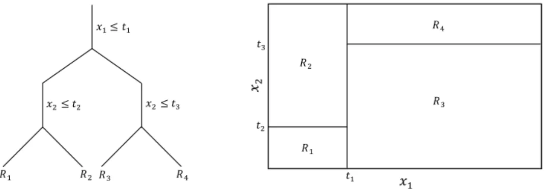
Friedman (2001) suggests a slight modifcation to Algorithm 2.1 when regression trees are used as the base learner function. Regression trees are a simple yet powerful tool that partition the feature space into a set of J non-overlapping rectangles and attach a simple constant to each one. The base learner function of a J-terminal node regression tree can be written as

J X

b(xt−k;{cj, Rj}Jj=1) = cjI(xt−k∈Rj), (2.7) j=1

where the functional estimate is a constant cj in region Rj. According to

Friedman (2001), the additive J-terminal node regression tree in equation (2.7) can be seen as a combination of J separate base learner functions. One base learner for each terminal node of the regression tree. Therefore after estimating the terminal node regions {Rjm}Jj=1at the mth iteration with least

squares on line 4 of the Algorithm 2.1 the line search step on line 5 should produce separate estimates for each terminal node of the regression tree. This minimization problem can be written as

N

J

X X

{cˆjm}Jj=1 =argmin L yt, Fm−1(xt−k) + cjI(xt−k∈Rjm) . (2.8)

{cj}Jj=1 t=1 j=1

The ensemble update on the last line of Algorithm 2.1 is then a sum of these J terminal node estimates obtained in equation (2.8)

J X

Fm(xt−k) =Fm−1(xt−k) + cˆjmI(xt−k∈Rjm).

j=1

2.2.2 Cost-sensitive gradient boosting with class weights

With a high class imbalance there is a risk that the estimated binary classifer is skewed towards predicting the majority class well (He and Garcia, 2009). An algorithm can be made cost-sensitive by weighting the dataspace according to the misclassifcation costs (Branco, Torgo and Ribeiro, 2016). This weighting approach is sometimes referred to as rescaling in the previous literature (see e.g., Zhou and Liu, 2010). The asymmetric misclassifcation costs, which are the building block of cost-sensitive learning, are incorporated to the gradient boosting model by introducing a binary class weight for each observation in the data. In the traditional gradient boosting model the sample counterpart of the loss function is the sample mean and the minimization problem can be written as in equation (2.6). By introducing a vector of class weights we end up minimizing the weighted average of the sample loss function

N M X X 1 min _N wtL yt, δmb(xt−k;γm) . (2.9) {δm,γm m}M=1 P _{t=1 m=1} wt t=1

If the weights wt are equal for each observation the weighted average in

equation (2.9) reduces to the sample mean.

Elkan (2001) suggests weighting the minority class observations according to the ratio in misclassifcation costs. Suppose c10denote the cost when we fail

to predict a recession and c01when we give a false alarm of recession. The

optimal weight for the minority class observations is then

∗ c10

w = . (2.10)

c01

In many cases the exact misclassifcation costs are unknown and we must rely on rules such that misclassifying the minority class is more costly (Maloof, 2003). The class weights are basically arbitrary as they depend on the unknown preferences how harmful different types of misclassifcation is considered to be. In this paper we use the data-based approach by Zhou (2012) and choose the weights according to the class imbalance observed in the dataset

⎧ _PN ⎪ ⎨ t=1(1 −yt) PN , if yt= 1 wt= _t=1yt . (2.11) ⎪ ⎩ 1, if y_t= 0

As can be seen from equation (2.11) the weights depend on the ratio of the number of datapoints in both classes. These binary weights ensure that the sum of weights are equal in both classes. The aim of choosing these weights is to force the algorithm to provide a balanced degree of predictive accuracy between the two classes.

The cost-sensitive gradient boosting algorithm with class weights follows the steps described in Algorithm 2.1 but the binary class weights can have an effect on each step of the algorithm. Table 2.1 illustrates how the class weights alter different parts of the gradient boosting algorithm, when J-terminal node regression trees are used as the base learner functions and the loss function to be minimized is the binomial deviance.

Table 2.1: The effect of class weights on the gradient boosting algorithm Step Value Loss function −2 PN t=1wt[ytF(xt−k)−log(1+eF(xt−k))] PN t=1wt

Initial value F0(xt−k)=log(

PN t=1wtyt PN t=1wt(1−yt) ) Gradient y˜tm=yt−pt, where pt= 1 1+e−Fm−1(x_t−k) Split criterion i2_(R l,Rr)= _WW_l+lW_Wr_r(¯gl−¯gr)2, Wl= P xt−k∈Rl wt ¯ gl= _W1_l P xt−k∈Rl wty˜tm Terminal node estimate ˆcjm = P xt−k∈Rjwt(yt−pt) P xt−k∈Rjwtpt(1−pt)

Note that the values for each step of the ordinary gradient boosting model can be obtained from Table 2.1 by setting all the weights equal to one. The cost-sensitive and the traditional gradient boosting algorithms differ starting from the initial values. As the frst gradient vector is based on the initial value the gradients are also different. The biggest differences between these two algorithms however are related to the estimation of the regression tree base learners at each iteration mof the algorithm. Blagus and Lusa (2017) argue that the class imbalance problem of the gradient boosting model with high-dimensional data is related to the inappropriately defned terminal regions

Rj.

Next we will consider how class weights can have an effect on both the estimated terminal node regions and the terminal node estimates of the re-gression tree base learner. When J-terminal node regression tree is used as the base learner function, the J −1recursive binary splits into regions Rland

Rrdividing the predictor space into J non-overlapping terminal node regions

{Rj}Jj=1are obtained by maximizing the least-squares improvement criterion.

These splits are based on a slightly different criterion if class weights are used. For this reason the estimated terminal node regions and the terminal node estimates can be different between the two algorithms.

The frst part WlWr _{illustrates how each split into regions R}

l and Rr in Wl+Wr

cost-sensitive gradient boosting is based on the sum of weights in these two categories instead of the number of observations. The latter part of the split criterion (¯gl−g¯r)2 shows that instead of the average gradient we compare

the weighted average of the gradient in the regions, when searching for the optimal split point. From the last row in Table 2.1 one can note how the terminal node estimates are functions of both the terminal node regions and the class weights itself and hence the fnal estimates can be different between the two algorithms.

2.2.3 Regularization parameters in gradient boosting

Friedman (2001, 2002) introduces several add-on reqularization techniques to reduce the risk of overftting or to improve the overall performance of the gradient boosting algorithm. The parameters related to these techniques are often called tuning parameters since it is up to the user to fnetune the parameter values for the particular problem at hand. Tuning parameters with the gradient boosting technique can be divided into two categories: parameters related to the overall algorithm and parameters related to the chosen base learner function.

Friedman (2001) incorporates a simple shrinkage strategy to slow down the learning process. In this strategy each update of the algorithm is scaled down by a constant called learning rate. The ensemble update on the last line of Algorithm 2.1 can then be written as

Fm(xt−k) =Fm−1(xt−k) +υρmb(xt−k;γm),

where 0 < υ ≤ 1is the learning rate. Learning rate is a crucial part of the gradient boosting algorithm as it controls the speed of the learning process by shrinking each gradient descent step towards zero. Friedman (2001) sug-gests to set the learning rate small enough for better generalization ability. Bühlmann and Yu (2010) reach a similar conclusion.

Breiman (1996) notes that introducing randomness when building each tree in an ensemble can lead to substantial gains in prediction accuracy. Based on these fndings Friedman (2002) develops stochastic gradient boosting in which subsampling is used to enhance the generalization ability of the

gradi-ent boosting model. At each round of the algorithm a random subsample of datapoints is drawn without replacement and the new base learner function is ftted using this random subsample. Simulation studies show that subsam-pling fraction around one half seems to work best in most cases (Friedman, 2002).

The total amount of iterations M needed however moves in the opposite direction to learning rate and subsampling. Gradient boosting is a fexible technique which can approximate basically any kind of functional form with suffcient amount of data. This fexibility can also come with a cost. Overftting the training data is a risk that must be taken into consideration as it can lead to decreased generalization ability of the model. The optimal amount of iterations is usually chosen with early stopping methods such as using an independent test set or cross-validation.

When the amount of observations is scarce K-fold cross-validation is often the only alternative since we can not afford to set aside an independent test set. K-fold cross-validation is based on splitting the data into Knon-overlapping folds. Each of these folds is used as a test set once while the model is estimated using the remaining K−1folds. To reduce the effect of randomness the K-fold cross-validation process can be repeated Rtimes (Kim, 2009). In the repeated K-fold cross-validation approach the estimate for the optimal stopping point is based on the average validation error produced by the Kfolds at each of these Rrepeats.

Instead of the traditional repeated K-fold we use a more conservative cross-validation approach since the risk of overftting the data in the high-dimensional setup is fairly high. In this conservative approach only the validation error produced by the fold, which frst reaches its minimum and therefore frst starts to show signs of overftting, is selected out of the K folds at each repetition. By denoting the found "weakest" fold in repetition r as kr∗, the number of observations in this fold as Nkr∗ and the model estimated

F−k∗

without this fold as ˆ r_(x

t−k)the conservative cross-validation estimate for

the prediction error can be written as

Nk∗ X X _� 1 R 1 r Fˆ−k∗ CV = L yt, r(xt−k) , (2.12) R_r=1 Nkr∗ _t=1

where binomial deviance is used as the loss function L(·). The fnal estimate for the amount of iterations is the point where the estimated prediction error in (2.12) reaches its minimum. To the best of our knowledge this simple conservative approach has not been used in the previous academic research.

The complexity of the regression tree base learners is controlled by the number of terminal nodes J in each regression tree. The amount of inner nodes (J −1)in the regression tree limit the potential amount of interaction between predictors as shown with the ANOVA expansion of a function

X X X

F(xt−k) = fj(xj) + fjk(xj, xk) + fjkl(xj, xk, xl) +· · · . (2.13)

j j,k j,k,l

The simplest regression tree with just two terminal nodes can only capture the frst term in equation (2.13). Higher order interactions are needed to be able to capture the latter terms, which are functions of more than one variable. These higher-order interactions require deeper trees. Hastie, Tibshirani and Friedman (2009) argue that trees with more than ten terminal nodes are seldom needed with boosting.

2.3 Results

2.3.1 Data and model setup

The dataset used in the empirical analysis is the FRED-MD monthly dataset. The selected timespan covers the period from January 1962 to June 2017. After dropping out variables that are not available for the full period the FRED-MD dataset consists of 130 different economic and fnancial variables related to different parts of the economy.1 Three different forecasting horizons hare studied in the empirical analysis: short (h = 3), medium (h = 6) and long (h=12).

All the available lag lengths kof the predictors up to 24 months are consid-ered as potential predictors (assuming k≥h). The total amount of predictors in the dataset take the value of 2860, 2470 or 1690 depending on the length of

1 _{All ISM-series (The Institute for Supply management) have been removed}

from the FRED-MD dataset starting from 2016/6. These series have been re-obtained using Macrobond. For more general information about the dataset see https://research.stlouisfed.org/econ/mccracken/fred-databases/

the forecasting horizon. For example, the total amount of predictors with the shortest forecasting horizon is 2860, which includes 22 different lags of these 130 variables. See Christiansen, Eriksen and Møller (2014) for a similar study where each lag is considered as a separate predictor.

The term spread has been noted as the best single predictor of recessions and economic growth in general in the U.S. (see e.g., Dueker, 1997; Estrella and Mishkin, 1998; Wohar and Wheelock, 2009). To see if it is actually worthwhile to go through these huge predictor sets with the gradient boosting models, we use a simple logit model with the term spread as a benchmark model. Kauppi and Saikkonen (2008) note that setting the lag length kequal to the forecasting horizon hmay not be optimal in all cases. To take this into account we introduce the six nearest lag lengths of the term spread as additional predictors. The term spread is measured as the interest rate spread between the 10-year government bonds and the effective federal funds rate as this is included in the FRED-MD dataset.

The estimated conditional probabilities for different models are evaluated using the receiver operating characteristic curve (ROC). The area under the ROC-curve (AUC) measures the overall classifcation ability of the model without restricting to a certain probability threshold. AUC-values closer to one indicate better classifcation ability whereas values close to one half are no better than a simple coin toss. For a more comprehensive review of the AUC-measure in economics context see e.g., Berge and Jordà (2011) and Nyberg and Pönkä (2016).

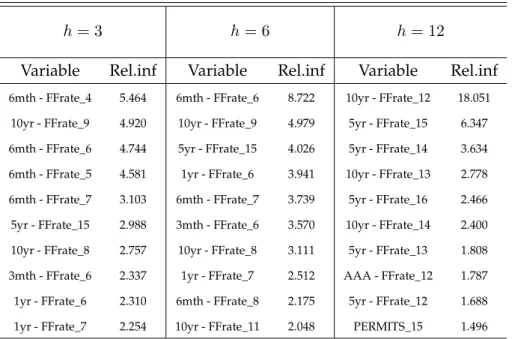
The gradient boosting model involves internal model selection as the regression trees selected at each step of the algorithm may be functions of different predictors. Some predictors are chosen more often than others and can be considered more important. Breiman et al. (1984) introduce a measure for the relevance of a predictor xp in a single J-terminal node regression tree

T

J−1

X

Iˆp2(T) = ˆı2_jI(vj =p), (2.14) j=1

where vjis the splitting variable of inner node jandˆıj2is the empirical

improve-ment in squared error as a result of this split. The least squares improveimprove-ment criterion was introduced in Table 2.1.

The measure in equation (2.14) is based on a single tree, but it can be generalized to additive tree expansions as well (Friedman, 2001). The relative infuence of a variable xpfor the entire gradient boosting ensemble is simply

an average over all the trees {T_m}M _{in the ensemble} m=1 M X 1 Iˆ_p2 = Iˆ_p2(Tm). (2.15) M m=1

The relative infuence measure in equation (2.15) is used to illustrate the most important recession indicators with the gradient boosting model. The relevance of a predictor xpin the recursive out-of-sample forecasting is the

average Iˆ_p2 of the estimated models.

The following results are obtained using the R programming environment for statistical computing (R Core Team, 2017). The GBM-package (Ridgeway, 2017) with bernoulli loss function is used to estimate the gradient boosting models. With such huge predictor sets it is likely that there are interaction between some predictors. For this reason the maximum tree depth is set to 8 leading to regression trees with nine terminal nodes. Döpke et al. (2017) use 6-terminal node regression trees while predicting recessions in Germany with a much smaller predictor set.

The minimum number of observations required in each terminal node of a regression tree is set to one allowing the tree building process to be as fexible as possible. Similar results are obtained when setting the minimum number of observations to fve as is used by Döpke et al. (2017).2 Learning rate is set to a low value of 0.005 and the default value of 0.5 is used as the subsampling fraction. The conservative cross-validation approach presented in equation (2.12) is conducted using 5 folds and 5 repeats throughout this research to fnd the optimal amount of iterations. In order to keep the computational time feasible the maximum amount of iterations is set to 800.

2.3.2 In-sample results

Three different models are compared in the in-sample analysis using the full dataset. The benchmark model (bm) is a simple logit model with seven lags of the term spread as predictors. GBM is the ordinary gradient boosting model

and wGBM stands for the cost-sensitive gradient boosting model with class weights. The class weights are formed according to equation (2.11). The binary response variable for each model is the business cycle chronology provided by the NBER.

Table 2.2 summarizes the in-sample performance as measured with the area under the ROC-curve (AUC) of these three models for all the different forecasting horizons. The rows of the table present the different models and the columns stand for the forecasting horizons considered. The validation AUCs from the 5-fold cross-validation repeated fve times are reported in parenthesis.

Table 2.2: In-sample AUC (1962/01 - 2017/06)

Forecast horizon, Months

Model specifcation 3 6 12

Benchmark 0.890 (0.881) 0.910 (0.902) 0.914 (0.897)

GBM 1.000 (0.985) 1.000 (0.980) 1.000 (0.956)

wGBM 1.000 (0.987) 1.000 (0.981) 1.000 (0.961)

As expected, the non-linear gradient boosting models do a better job fore-casting recessions in-sample. The larger information set and the more fexible functional form of the GBM-models allow for a more detailed in-sample ft. The perfect in-sample AUCs for the GBM-models can raise questions of over-ftting. As a result of using these moderate sized regression trees as base learner functions the GBM-models achieve nearly perfect classifcation ability after only a few iterations. This can be confrmed by training a shallow single decision tree to the full dataset. The single decision tree alone is suffcient to produce very high in-sample AUCs, even after restricting the predictor space to consider only the eight different interest rate spreads (and their lag lengths).3 Thereby it is not completely surprising that an ensemble of trees

3 _{The in-sample AUCs with a single decision tree are close to or well above 0.95}

depend-ing on the forecastdepend-ing horizon. On the other hand, restrictdepend-ing the GBM-models by consid-ering only the simplest stump regression trees and / or only the interest rate spreads as predictors are not suffcient as models produce in-sample AUCs of one or really close to it. Results upon request.

yield a perfect in-sample ft as measured with AUC. For example, the cost sensitive GBM-model with the shortest forecasting horizon reaches an AUC value of 0.997 after just fve iterations. However it should be noted that the estimated conditional probabilites at this point range between 0.488 and 0.512, values that are only slightly different from the initial value of one half because of the shrinkage strategy described in Section 2.2.3. It could be argued that the AUC may not be the most suitable criterion when evaluating the in-sample performance in this setup. But since the main emphasis is on the out-of-sample performance of the models the AUCs are reported here for comparison.

The validation AUCs reported in Table 2.2 provide additional insight into the potential overftting problem since large deviations between the in-sample and validation performance is typically seen as a sign of overftting. The vali-dation AUCs for the GBM-models are of similar magnitude as the in-sample AUCs and therefore do not indicate overftting. Döpke et al. (2017) also report validation AUCs close to one when forecasting recessions in Germany with the gradient boosting model. The validity of the traditional random sampling techniques used in cross-validation with such a highly autocorrelated binary response variable should be further examined. This however is beyond the scope of this research.

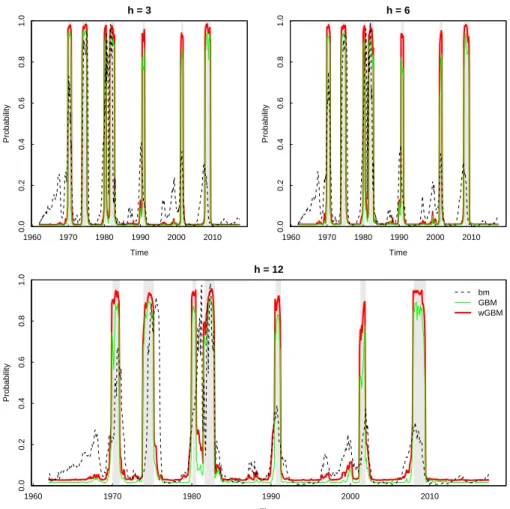
Table 2.2 shows how the cost sensitive GBM-model outperforms the other two models as measured with the validation AUC, although the difference between the two GBM-models is small. The gap in validation AUCs between the benchmark and GBM-models decreases slightly as the forecasting horizon grows. Graphical illustrations are an important part of recession forecasting since these can give a better picture of the false alarms and other potential problems related to the models. The estimated conditional probabilities that the economy is in recession h-months from now are calculated according to equation (2.2). These in-sample estimated conditional probabilites are illustrated in Figure 2.1 for each of the three models and forecasting horizons.