Runtime monitoring of Java programs by Abstract State Machines

Runtime monitoring of Java programs by Abstract State

Machines

Paolo Arcaini

Universit`

a degli Studi di Milano

Angelo Gargantini

Universit`

a degli Studi di Bergamo

Elvinia Riccobene

Universit`

a degli Studi di Milano

1

Introduction

Runtime software monitoring has been used for software fault-detection and recovery, as well as for profiling, optimization, performance analysis. Software fault detection provides evidence that program behavior conforms or does not conform with its desired or specified behavior during program execution. While other formal verification techniques, such as model checking and theorem proving, aim to ensure universal correctness of programs, the intention of runtime software-fault monitoring is to determine whether the current execution behaves correctly; thus, monitoring aims to be a lightweight verification technique that can be used to provide additional defense against failures and confidence of the system correctness.

Runtime monitoring should be considered when you cannot execute an exhaustive verification of your system (in most of the cases); for example, proving a security property that your system never reaches a dangerous state could require too much time depending on the size of your system. On the contrary, testing could be considered not enough trustworthy, in particular in critical systems. Moreover there could be some information that are available only at run-time, or the behaviour of the system could depend on the (not reproducible) environment where the system runs. Finally it could also be possible that, nevertheless the system has been tested and maybe also proved correct, the developer wants to be sure that the system does not violate some given properties during its execution. Extending the thought of Ed Brinksma, expressed during the 2009 keynote at the Dutch Testing Day and Testcom/FATES, on the relationship between verification and testing1, we could ask:

Who would want to fly in an airplane with software proved correct, hardly tested, but not monitored at run-time?

In most approaches dealing with run time monitoring of software, the required behavior of the system is formalized by means of correctness properties [8] (often given as temporal logic formulae) which are then translated into monitors. The monitor is then used to check the execution of a system if the properties are violated. The properties specify all admissible individual executions of a system and may be expressed using a great variety of different formalisms. These range from, for example, language oriented formalisms like extended regular expressions or tracematches by the AspectJ team. Temporal logic-based formalisms, which are well-known from model checking, are also very popular in runtime verification, especially variants of linear temporal logic, such as LTL, as seen for example in [10, 3]. For an overview about runtime verification techniques and tools, please refer to [14, 8, 7].

In this paper, we assume that the desired behavior of the system is given by means of Abstract State Machines (ASMs) which specify the behavior of the system in an operational way: they describe the desired changes of the system state when some particular input conditions occur. A similar approach is taken also in [15], where the specification is given in the Z language, which de-scribes the system states and the ways in which the states can be changed. Note that our approach requires a shift from adeclarativestyle of monitoring (based on properties) to anoperationalstyle, based on ASMs. Anoperationalspecification describes the desired behavior by providing a model implementation or model program of the system, generally executable. Examples of operational specifications are abstract automata and state machines. Another different specification style is through descriptive specifications, which are used to state the desired properties of a software component by using a declarative language. Examples of such notations are logic formulae, JML [13] or the LTL temporal logic. Different specification styles (and languages) may differ in their expressiveness and very often their use depends on the preference and taste of the specifier, the availability of support tools, etc. Up to now, descriptive languages have been preferred for run time software monitoring, while the use of operational languages has not been investigated with the same strength.

In this paper we assume that the implementation is a Java program, while the specification is an Abstract State Machine (ASM), whose notation is presented in section 2. In section 3 we present out theoretical framework, in which we explain the relationship between the Java implementation and the ASM specification. This relationship defines syntactical links or mappings between Java and ASM elements and a semantical relation which represents the conformance. The important issue of non-determinism is tackled in section 4. In section 5 we introduce the actual implementation of our monitoring approach which is based on Java annotations and AspectJ. In section 6 we show how our monitoring system can be used in practice through the illustration of some examples.

2

Abstract State Machines

Abstract State Machines (ASMs), whose complete presentation can be found in [5], are an exten-sion of FSMs [4]. Machinestates are multi-sorted first-order structures, i.e. domains of objects with functions and predicates (boolean functions) defined on them, and thetransition relation is specified by “rules” describing how functions change from one state to the next.

Basically, a transition rule has the form ofguarded update “if ConditionthenUpdates” where Updates are a set of function updates of the form f(t1, . . . , tn) := t which are simultaneously

executed whenCondition is true. f is an arbitrary n-ary function andt1, . . . , tn, tare first-order

terms.

To fire this rule in a state si, i≥0, all terms t1, . . . , tn, t are evaluated atsi to their values,

say v1, . . . , vn, v, then the value of f(v1, . . . , vn) is updated to v, which represents the value of

f(v1, . . . , vn) in the next state si+1. Such pairs of a function name f, which is fixed by the

signature, and an optional argument (v1, . . . , vn), which is formed by a list of dynamic parameter

valuesviof whatever type, are calledlocations. They represent the abstract ASM concept of basic

object containers (memory units), which abstracts from particular memory addressing and object referencing mechanisms. Location-value pairs (loc, v) are called updates and represent the basic units of state change.

There is a limited but powerful set of rule constructors that allow to express simultaneous parallel actions (par) or sequential actions (seq). Appropriate rule constructors also allow non-determinism (existential quantificationchoose) and unrestricted synchronous parallelism (univer-sal quantificationforall).

A computation of an ASM is a finite or infinite sequence s0, s1, . . . , sn, . . . of states of the

machine, wheres0 is an initial state and each sn+1 is obtained from sn by firing simultaneously

all of the transition rules which are enabled insn. The (unique)main rule is a transition rule and

represents the starting point of the computation. An ASM can have more than oneinitial state. A stateswhich belongs to a computation starting from an initial state s0, is said to bereachable

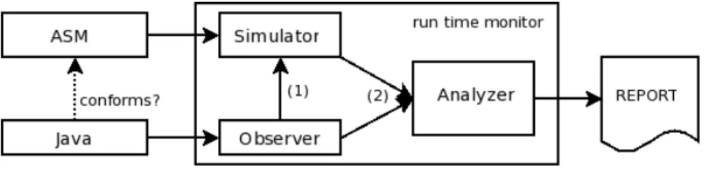
Figure 1: A runtime monitor for Java

For our purposes, it is important to recall how functions are classified in an ASM model. A first distinction is betweenbasic functions which can bestatic (never change during any run of the machine) ordynamic (may be changed by the environment or by machine updates), andderived functions, i.e. those coming with a specification or computation mechanism given in terms of other functions. Dynamic functions are further classified into: monitored (only read, as events provided by the environment),controlled (read and write (i.e. updated by transaction rules)), shared and output (only write) functions.

The ASMETA tool set [1] is a set of tools around the ASMs. Among them, the tools involved in our monitoring process are: the textual notationAsmetaL, used to encode fragments of ASM models, and the simulatorAsmetaS, used to execute ASM models.

3

Runtime monitoring based on ASM specifications

Aruntime software-fault monitor, or simply amonitor, is a system that observes and analyzes the states of an executing software system. The monitor checks correctness of the system behavior by comparing anobserved state of the system with an expected state. The expected behavior is generally provided in term of a formal specification. In this paper, we intend runtime monitoring as conformance analysis at runtime.

Depending if the monitor is designed to consider executions in an incremental fashion or to work on a (finite set of) recorded execution(s), a monitor allowsonline monitoringoroffline monitoring, respectively [14].

The monitor we propose, which allows online monitoring, takes in input an executing Java software system and an ASM formal model written in AsmetaL. The monitor observes the behavior of the Java system and determines its correctness w.r.t. the ASM specification working as an oracle of the expected behavior. While the software system is executing, the monitor checks conformance between the observed state and the expected state.

As shown in Fig. 1, the monitor is, therefore, composed of: anobserverthat evaluates when the Java (observed) state is changed, and leads the abstract ASM to perform a machine step, and an analyzer that evaluates the step conformance between the Java execution and the ASM behavior. When a violation of conformance is detected, it quits the monitoring upon the user request.

We here focus only on monitors that are used to detect faults, which occur during the execution of software and results in an incorrect state. Other monitoring systems extend this capability by diagnosing faults, i.e., providing information to the user that will aid the user in understanding the cause of the fault and assist the system in recovering from faults by directing the system to a correct state (forward recovery) or by reverting to a state known to be correct (backward recovery). In the following sections, we pose the theoretical bases of our monitoring system. We, therefore, formally define what is an observed Java state, how to establish a conformance relation between Java and ASM states, and, therefore, step conformance and runtime conformance between Java and ASM executions. Initially, we assume that either the Java program and the ASM model are deterministic. Non-determinism is dealt in section 4.

3.1

Observable Java elements and their link with ASM entities

In order to mathematically represent a Java class and the state of its objects, we introduce the following definitions.

Definition 1. ClassAclassC is a tuplehc, f, miwherec denotes the non-empty set of construc-tors,f is the set of all the fields,m is the set of methods.

We denote the public fields ofCasfpubwhile the public methods are denoted asmpub. Among the methods of a class, we distinguish also thepure methods (as in JML [13]):

Definition 2. Pure methodPure methods are side effect free, with respect to the object/program state. They return a value but do not assign values to member variables. mpub

pure denote the set of

all pure public methods inm.

Definition 3. Virtual State Given a classC =hc, f, mi, the virtual state, VS(C), is given by VS(C) =fpub_∪mpub

pure.

Definition 4. Observed StateWe define observed state,OS(C)⊆V S(C), as the subset of the virtual state consisting of all public fields, and pure public methods of the classC the user wants to observe.

Therefore,OS(C) is the set of Java elements monitored at runtime. For convenience, we can seeOS(C) =OF(C)∪OM(C) to distinguish between the subsetobserved fields OF(C) and the subset ofobserved methods OM(C) of OS(C). Note that OF(C) ⊆fpub andOM(C)⊆mpubpure.

Elements ofOS(C) can change by effect of the class method computation. Only methods inm¬pure

may change the program state.

Definition 5. Changing MethodGiven a Java classC, we define changing methods,

changingMethods(C)⊆m¬pure, all methods ofCwhose execution is responsible of changingOS(C)

and that the user wants to observe.

3.1.1 Linking observable Java elements to ASM entities

In order to be run-time monitored, a Java classC =hc, f, mi should have a corresponding ASM model,ASMC, abstractly specifying the behavior of an instance of the classC.

Observable elements of a classC must be linked to the dynamic functionsFuncs ASMC of the

ASM modelASMC. The function

link :OS(C)→Funcs ASMC (1)

yields the set of the ASM dynamic functions linked to the observable Java elements of C. The functionlinkis not surjective because there are ASM dynamic functions that are not used in the conformance analysis. Moreover, the function is not injective, because more than one Java field or method can be linked to the same ASM function.

3.2

Common representation of Java and ASM values

In order to be compared, Java values and ASM values must be translated into a common format. Let us consider a Java classC and the corresponding modelASM(C). The following functions, cfJ andcfA, provide string representations of, respectively, Java and ASM values, in a given state.

cfJ :OS(C)×SJ ava→String

cfA:ASM(C)×SASM →String

The first functioncfJ exploits the built-in Java functiontoString of the class Object. A similar function is provided by the ASMETA simulator to convert type values into strings for ASM models.

cfJ function Letebe a Java field or non-void method whose type ist. Letv_{J ava}j be the value ofein statesj_{J ava}.

The behaviour of thecfJ function depends on the type t; iftis

• a primitive type, an array, a String, a List, or a Set, its string representation in statesj_{J ava}

is

cfJ(e, sj_{J ava}) =vj_{J ava}

• a M ap < T, E > type2_{, we can identify with {k}1

J avaj, . . . , km_{J ava}j} the keys (of type T) of the map in the state sj_{J ava}, and {v1

J avaj, . . . , v_{J ava}m j} their corresponding values. The representation of the map in statesj_{J ava}is

cfJ(e, sj_{J ava}) ={k_{J ava}1 j →v1_{J ava}j, . . . , k_{J ava}m j →vm_{J ava}j} where parentheses, commas and arrows must be interpreted as strings.

cfA function Letf be a function name and{(v1

1, . . . , vn1)sk

ASM, . . . ,(v

m

1 , . . . , vmn)sk

ASM}the list of arguments values which identify the defined locations (that is the locations whose value is different from undef) in state sk

ASM ; moreover let {v1sk ASM

, . . . , vm sk

ASM

} the values in the current state

sk_ASM of the locations {f(v₁1, . . . , v1_n)sk

ASM, . . . , f(v

m

1 , . . . , v

m n)sk

ASM}. The string representation of the n-ary functionf in statesk

ASM is cfA(f, sk_ASM) ={(v₁1, . . . , v_n1)_sk ASM →v 1 sk ASM , . . . ,(vm₁ , . . . , v_nm)_sk ASM →v m sk ASM }

where parentheses, commas and arrows must be interpreted as strings.

If f is a 0-ary function, it has just one location (if defined). The value of the location in the statesk isvsk. The string representation of the 0-ary functionf in statesk is

cfA(f, sk) =vsk

3.3

Execution step in Java and ASM

In order to define a step of a Java class execution, we heavily rely on the concept ofmachine step andlast state of execution sequence defined in the Unifying Theories of Programming (UTP) [11]. Thestep is defined as a relation between the virtual state before the step and the virtual state after. In the case of an execution of a Java method, the state can be analyzed as a pair (s;m), wheres is the data part (actual values of the variables), andmis a representation of the rest of the method code that remains to be executed. When this is Π, there is no more method code to be executed; the state (t; Π) is thelast state of any execution sequence that contains it, andtdefines the final values of the variables.

Definition 6. Java StepLetmbe a method of a Java class. A Java step is defined as the relation (s, m)J step→ (s0,Π), where s is the starting state of the execution ofm ands0 the last state of this execution.

In the sequel, we abbreviate (s, m)J step→ (s0,Π) with (s, m, s0).

Definition 7. Change Step Let C be a Java class. A change step is defined as Java step for

m∈changingMethods(C).

ASMstate and ASM computationstep have been defined in section 2.

ASMC init// S0 +3Sj step _// Sj+1 step _// C inst//s0 O O + 3sk O O notCM_{/o /o /o //} s0_k _ _ CM_//s k+1 O O

Figure 3: Runtime conformance

3.4

State Conformance, Step Conformance and Run Conformance

We have formally related a Java class and its execution(s) with the corresponding abstract ASM model and relative execution(s). In the following definitions, letC be a Java class andASMC its

corresponding ASM abstract model.

Definition 8. State ConformanceWe say that a statesof Cconforms to a state S of ASMC

if all observed elements ofC have value string representation equal to the string representation of the values of the locations in ASMC linked to them; i.e.

conf(s, S)≡ ∀e∈OS(C) :cfJ(e, s) =cfA(link(e), S) (2)

Definition 9. Step Conformance We say that a change step (s, m, s0_{)of C, withm a method}

ofC,conforms with a step (S, S0)of ASMC if conf(s,S)∧conf(s0,S0).

Definition 10. Run time conformanceGiven an observed computationof a Java classC, we say thatC is run time conformingto its specification ASMC if the following conditions hold:

• the initial states0of the computation ofC conformsto the initial stateS0of the computation

of ASMC, i.e. it yields conf(s0, S0);

• every observed change step (s, m, s0) with s the current state of C, conforms with the step (S, S0)of ASMC withS the current state of ASMC.

ASM: ASMC S step _// S0 Java class: C s O O m _// s0 O O

Figure 2: Step conformance This definition presumes there exists a

com-putation of the classC one can observe. Fur-thermore, it assumes that the next state of C

and of its specificationASMC are unique, thus

it assumes determinism of the system under monitoring. Non-deterministic computations are considered in the next section.

Due to the run-time conformance definition between a Java class and its ASM specification,

the final state of a Java change step and the initial state of the subsequent change step are both state conforming to the same abstract state of the ASM (see Fig.3).

4

Dealing with Non-determinism

Definition 10 assumes that, in any computation, the next state of a Java classC and of its spec-ification ASMC are unique. Thus, the definition is adequate for deterministic systems:

non-determinism is limited to monitored quantities, which, once non deterministically fixed by the environment, make the evolution of the system deterministic. In this section, we extend our con-ceptual framework to deal with non-determinism alsoinside the system (in the classC and/or in the specificationASMC). We have identified the following non-deterministic situations:

• Non-deterministic Java class and non-deterministic ASM specification. This situation can be due to one of the following scenarios:

– a class changing method has non-deterministic behavior, and so, therefore, the abstract specification. For instance, it contains a call to a method in the java.util.Random class;

– the Java class has more then one changing method, each of which may be deterministic; however, it is non-deterministic the choice of the changing method that causes a change step. The abstract ASM model should capture this non-determinism and assure that the behavior of the methods is correct and that calling sequences are those permitted.

• Deterministic Java class and non-deterministic ASM specification. This situation can be due to an underspecification of the ASM model which may result more abstract (with less implementation details) than the corresponding Java code and possibly non-deterministic. In caseC or ASMC are non-deterministic, the next computational state of Cor ASMC is not

always uniquely determined, and, therefore, their conformance, according to definition 10, may fail not because of a wrong behavior of the implementation, but becauseC andASMC may choose a

different non-conformant next state. We here refine definition 10 of step conformance and run-time conformance in case of non-determinism, distinguishing between weak and strong conformance.

4.1

Weak and strong conformance

For theweak conformance, we require that the next step ofC is state-conforming with at least oneof the next states of the specificationASMC. For the strong conformance, we require that the

next step ofC is state-conforming withone and only one of the next states of the specification. Formally:

Weak run time conformance We say thatCisweaklyrun time conforming to its specification ASMC if the following conditions hold:

• the initial states0 of the computation ofC conforms toat least one initial state S0 of the

computation ofASMC, i.e. ∃S0 initial state ofASMC such thatconf(s0, S0);

• for every change step (s, m, s0) withsthe current state ofC,∃(S, S0) step of ASMC withS

the current state ofASMC, such that (s, m, s0) isstep conforming (S, S0).

Strong run time conformance We say thatC is strongly run time conforming to its specifi-cationASMC if the following conditions hold:

• the initial states0 of the computation ofCconforms toone and only one initial stateS0of

the computation ofASMC, i.e. ∃!S0initial state ofASMC such thatconf(s0, S0);

• for every change step (s, m, s0) withsthe current state ofC,∃! (S, S0) step ofASMC withS

the current state ofASMC, such that (s, m, s0) isstep conforming (S, S0).

Currently, our monitoring system can only deal with strong conformance. In case of nonde-terministic ASM, during the runtime monitoring our system chooses, among the next states of the ASM, the state that is compliant with the Java state. If there is more than one state (weak conformance), the system does not know which one to choose. The feature of weak conformance is not supported for the moment, and a violation is risen since we require thatC must be strong conformant withASMC. Weak conformance will be considered for future work.

5

Monitor Implementation

We here describe how our system works for the ASM-based runtime monitoring of Java programs. We provide technical details on how the observer and the analyzer have been implemented by exploiting the mechanism of the Java annotations to link observable Java elements to corresponding ASM entities, and the support of external tools as AspectJ to establish the conformance relation.

5.1

Using Java Annotations

Annotationsare meta-data tags that can be used to add some information to code elements as class declarations, field declarations, etc. Each annotation have aRetentionPolicy that signals how and when the annotation can be accessed; Runtime policy, for example, signals that the annotation can be read by the compiler and can also be read reflectively at run-time.

In addition to the standard ones, annotations can be defined by the user similarly as classes. For our purposes we have defined a set of annotations in order to link the Java code to its abstract specification. The retention policy of all of our annotations isruntime since we need to read them reflectively while the program is running.

5.1.1 Our annotations

Our use of the annotation mechanism requires a very limited code modification and differs from that usually exploited in other approaches for system monitoring. Usually annotations are used to enrich the code with extra formal specification to obtain dynamic information about the target program [6, 12]. This leads to the lack of separation between the implementation of the system and its high-level requirements specification. In our approach, the few annotations are only used to link the code to its specification, but keeping them separately. This allows the reuse of a highly abstract formal requirement specification when changes happen to the implementation of the target system. Furthermore, annotations are statically type checked and since the annotations are read reflectively at run time, the monitoring setup can be carried out very easily. We found this approach much more convenient than inserting special comments (like JML) and writing our own parser for them.

Let’s see in details each annotation.

@Asm In order to link a Java class C with its corresponding ASM model ASMC, the Java

class must be annotated with the @Asm annotation having the path of the ASM model as string attribute. The Java class EuclidGCD (see code 1) specifies, as its ASM specification, the model shown in code 2.

package e u c l i d ;

import o r g . asmeta . m o n i t o r i n g . Asm ;

import o r g . asmeta . m o n i t o r i n g . F i e l d T o F u n c t i o n ;

import o r g . asmeta . m o n i t o r i n g . I n i t ;

import o r g . asmeta . m o n i t o r i n g . RunStep ;

import o r g . asmeta . m o n i t o r i n g . S t a r t M o n i t o r i n g ; @Asm( a s m F i l e=” models / euclidGCD . asm” )

public c l a s s EuclidGCD { @FieldToFunction ( f u n c=”numA” ) public i n t numA ; @FieldToFunction ( f u n c=”numB” ) public i n t numB ; @ S t a r t M o n i t o r i n g

public EuclidGCD ( @ I n i t ( f u n c=” initNumA ” ) i n t a , @ I n i t ( f u n c=” initNumB ” ) i n t b ) {

numA = a ; numB = b ;

}

public i n t getGCD ( ) {

while(numA != numB) {

}

return numA ;

}

@RunStep

private void euclidGCDstep ( ) {

i f(numA > numB) {

numA = numA − numB ;

} e l s e {

numB = numB − numA ;

} } }

Code 1: GCD Java code

asm euclidGCD

import . . / . . / . . / . . / asm examples /STDL/ S t a n d a r d L i b r a r y

signature:

dynamic c on t ro ll e d numA : I n t e g e r

dynamic c on t ro ll e d numB : I n t e g e r

dynamic monitored initNumA : I n t e g e r

dynamic monitored initNumB : I n t e g e r

d e f i n i t i o n s:

main rule r Main =

i f(numA != numB) then i f(numA > numB) then

numA := numA − numB

e l s e

numB := numB − numA

endif endif

d e f a u l t i n i t s 0 :

function numA = initNumA

function numB = initNumB

Code 2: GCD ASM model

@FieldToFunction and @MethodToFunction To establish the mapping defined by the

func-tionlinkwe must annotate each observed fieldf ∈OF(C) and each observed methodm∈OM(C). The fields that are linked to controlled functions are annotated by @FieldToFunction, while the observed methods by @MethodToFunction; both these annotations have a string attribute yielding the name of the corresponding ASM controlled function.

In code 1 a Java code that computes the greatest common divisor (GCD) through the Euclidean algorithm is shown; an equivalent ASM model is shown in code 2. We can see that the Java fields numAandnumB are linked with two homonymous ASM controlled functions.

Both @FieldToFunction and @MethodToFunction annotations are used to indicate some con-trolled functions of the ASM specification. The @FieldToFunctioncreates a direct connection

between a field and a function. The @MethodToFunctionannotation, instead, permits to create more complicated links: the comparison is made between the value returned by the annotated method and the value of the referenced function. In this way we can link an ASM function with any computation of the Java code (operations between fields, method calls, . . . ).

The linking between the Java state and the ASM state can be made:

• using only @FieldToFunctionannotations,

• using only @MethodToFunctionannotations,

• or using both together3.

Moreover there are no restrictions on the number of variables and methods by which an ASM function is referenced.

It’s important to notice that, if it’s not possible to establish a link between a field and a function (with the @FieldToFunctionannotation)4_{, we can establish the link through a getter}

method (annotated with the @MethodToFunction annotation) whose return value is compatible with the intermediate format of the ASM location values. Let’s see, as an example, the Java code shown in code 3 and the ASM model shown in code 4. They both model a door which is, alternatively,open orclosed.

package o r g . asmeta . m o n i t o r i n g ; @Asm( a s m F i l e=” e x a m p l e s / d o o r . asm” )

public c l a s s Door { boolean doorIsOpen ; Door ( ) { doorIsOpen = f a l s e; } @RunStep public void s t e p ( ) { doorIsOpen = ! doorIsOpen ; } @MethodToFunction ( f u n c=” d o o r S t a t u s ” , a r g s = { }) S t r i n g getDoorIsOpen ( ) { i f( doorIsOpen ) { return ”OPEN” ; } e l s e { return ”CLOSED” ; } } }

Code 3: Door Java code

3_{We can notice that all the links made with the @FieldToFunction annotation can also be made with the}

@MethodToFunction annotation: we just have to create a getter method for the variable annotated with the @FieldToFunction annotation and annotate it with the @MethodToFunction annotation (using the same values of the @FieldToFunctionannotation, that is referencing the same function).

4_{It’s not possible to establish a link between a field and a function when the intermediate representations of their}

asm d o o r

import . . / . . / . . / . . / asm examples /STDL/ S t a n d a r d L i b r a r y

signature:

enum domain DoorStatusDomain = {OPEN | CLOSED}

dynamic c on t ro ll e d d o o r S t a t u s : DoorStatusDomain

d e f i n i t i o n s:

main rule r Main =

i f( d o o r S t a t u s = CLOSED) then d o o r S t a t u s := OPEN e l s e d o o r S t a t u s := CLOSED endif d e f a u l t i n i t s 0 : function d o o r S t a t u s = CLOSED

Code 4: Door ASM model

The Java code represents the door status with the boolean variableisOpen. The ASM model, instead, uses the functiondoorStatus, which takes values in the enum domain{OP EN, CLOSED}, to indicate if the door is open or not. We can observe that the Java code and the ASM model do the same thing, but the intermediate representations of the Java variableisOpen and of the function doorStatus values are not compatible. So we have written the method getIsOpen (annotated with the @MethodToFunctionannotation) which returns the string “OPEN” whenisOpen istrue, “CLOSED” otherwise.

@Monitored The fields whose values are determined at run time by the environment (e.g. values received by any kind of input stream) are linked to monitored ASM functions and they are annotated with @Monitored. These fields are used to give values to the corresponding ASM monitored functions before executing achanging method, as explained later in section 5.2. Let’s see, as an example, the Java code shown in code 5 and the ASM model shown in code 6. They both model an air conditioner that can be used with three speeds: 0 (turned off), 1 and 2. The speed depends on the temperature of the room. In the Java code the temperature is represented by the integer variableroomTemperature. This variable ismonitored because its value is determined by the environment, i.e. a sensor controlled by an object of the classTemperatureSensor.

In the ASM model the temperature is modeled through the monitored functiontemperature that can assume the values 0, 1 and 2.

The Java variableroomTemperature is linked with the monitored functiontemperature of the ASM model.

package c o n d i t i o n e r ;

import o r g . asmeta . m o n i t o r i n g . Asm ;

import o r g . asmeta . m o n i t o r i n g . F i e l d T o F u n c t i o n ;

import o r g . asmeta . m o n i t o r i n g . Monitored ;

import o r g . asmeta . m o n i t o r i n g . RunStep ;

import o r g . asmeta . m o n i t o r i n g . S t a r t M o n i t o r i n g ; @Asm( a s m F i l e=” models / a i r C o n d i t i o n e r . asm” )

@Monitored ( f u n c=” t e m p e r a t u r e ” , a r g s ={}) public i n t roomTemperature ; @FieldToFunction ( f u n c=” a i r S p e e d ” ) public i n t a i r I n t e n s i t y ; private T e m p e r a t u r e S e n s o r t s ; @ S t a r t M o n i t o r i n g public A i r C o n d i t i o n e r W i t h S e n s o r ( ) { a i r I n t e n s i t y = 0 ; t s = new T e m p e r a t u r e S e n s o r ( ) ; } public void c h e c k ( ) { readRoomTemperature ( ) ; s e t A i r I n t e n s i t y ( ) ; } @RunStep private void s e t A i r I n t e n s i t y ( ) { i f( roomTemperature < 2 0 ) { a i r I n t e n s i t y = 0 ; } e l s e i f( roomTemperature < 2 5 ) { a i r I n t e n s i t y = 1 ; } e l s e { a i r I n t e n s i t y = 2 ; } }

private void readRoomTemperature ( ) {

t h i s. roomTemperature = t s . readRoomTemperature ( ) ;

} }

Code 5: Air conditioner Java code

asm a i r C o n d i t i o n e r

import . . / . . / . . / . . / asm examples /STDL/ S t a n d a r d L i b r a r y

signature:

domain AirSpeedDomain subsetof I n t e g e r

dynamic c on t ro ll e d a i r S p e e d : AirSpeedDomain

dynamic monitored t e m p e r a t u r e : I n t e g e r

d e f i n i t i o n s:

domain AirSpeedDomain = {0 . . 2}

main rule r Main =

i f( t e m p e r a t u r e >= 2 5 ) then

a i r S p e e d := 2

e l s e

a i r S p e e d := 0 e l s e a i r S p e e d := 1 endif endif d e f a u l t i n i t s 0 : function a i r S p e e d = 0

Code 6: Air conditioner ASM model

@RunStep All methods ofchangingM ethods(C) are annotated with the @RunStepannotation. In the Euclidean algorithm example (code 1), the changing method iseuclidGCDstep() that exe-cutes a single step of the algorithm. In the air conditioner example (code 5), the changing method issetAirIntensity().

@StartMonitoring and @Init Finally, the user have to decide the starting point of the mon-itoring. The annotation @StartMonitoring is used to select a proper (not empty) subset of constructors5.

All or some constructor parameters (if any) can be annotated with the @Initannotation that permits to link a parameter with a monitored function (i.e. only read, as events provided by the environment) of the ASM model. This allows initializing the ASM model with the same values used to create the Java instance.

In the Java code of the Euclidean algorithm example (see code 1), in the constructor, the formal parametera is annotated with the@Init annotation that contains areference to the monitored functioninitNumA of the ASM model; in the same way the formal parameterb is linked to the monitored function initNumB. We can notice, indeed, that in the ASM model 2 the controlled functions numA and numB are initialized through the monitored functions initNumA and init-NumB: in this way the ASM model can be executed several times to compute the GCD of different couples of numbers.

5.2

Observer implementation through AspectJ

Theobserver is implemented through the facilities of AspectJ that permits to observe easily the execution of Java objects. AspectJ allows to specify different pointcuts, that are points of the program execution we want to capture; for each pointcut it is possible to specify anadvice, that is the actions that must be executed when a pointcut is reached. AspectJ permits to specify when to execute theadvice: beforeor after the execution of the code specified by the pointcut.

In the definitions of AspectJ pointcuts, it is possible to add method annotations: this feature has permitted us to define easily the points of a program execution where our monitoring system must perform some given jobs.

For our purposes, we have defined the following two pointcuts:

pointcutobjCreated():call(@StartMonitoring∗.new(..));

pointcutrunStepCalled():call(@RunStep∗ ∗.∗(..))

&& !cflowbelow(call(@RunStep∗ ∗.∗(..)));

TheobjCreatedpointcut captures the creation of an instance of a class that must be monitored;

runStepCalledcaptures the execution of achanging method (we do not consider changing methods

that are executed in the scope of other changing methods).

In particular, after a joint point that belongs to objCreated, the monitor executes an advice that initializes a simulator for the corresponding ASM machine. Before the execution of a join

5_{We do not consider the default constructor. If the class does not have any constructor, the user have to specify}

point that satisfiesrunStepCalled, an advice is executed that records the values of the monitored fields and executes a state conformance check. After this joint point, another advice is executed that sets the ASM monitored functions, simulates a step of the ASM and forces the analyzer to check again the state conformance.

5.3

Analyzer

The analyzer must execute the comparison between the Java and the ASM state. The values of the ASM functions are obtained through the facilities of the AsmetaS simulator (a simulator for ASMs [9]). The values of the Java fields and methods are obtained through reflection. This is the reason why we require that the methods in OM(C) must be side-effect free: these methods are called through reflection by our monitoring system and we do not want that their execution influence (change) the Java state.

The Java and the ASM values are both transformed in a String representation through the functionscf J andcf A(see section 3.2); so the conformance check is simply a string comparison.

6

Monitoring settings by examples

In the previous section we have described how it is possible to bind a Java class together with an ASM specification, how their runs are related and how (and when) the conformance analysis is executed.

In this section we want to show, by means of some examples, how the monitoring system can be used in practice. Indeed, based on the kind of Java class we want to monitor and on the kind of the ASM model we use as formal specification, we can identify different kinds of monitoring.

First of all, starting from the definitions given in section 4, we classify the Java classes and the ASM specifications according to their determinism/non-determinism.

Deterministic ASM specification A deterministic ASM specification is a specification that does not contain any choose rule. At each step there is just one possible update set and so just one possible next state.

Non-deterministic ASM specification A non-deterministic ASM specification is a specifica-tion that contains at least a choose rule. At each step there could be more than one possible update set and so more than one possible next state.

Internally non-deterministic/deterministic Java class Given a class C, let m be the set of its methods. We say that the class isinternally non-deterministic if ∃mi ∈ m that contains

non-deterministic statements (e.g. a method call on an object of the java.util.Random class). Oth-erwise, if !∃mi∈mthat contains non-deterministic statements, we say that the class is internally

deterministic.

Externally non-deterministic/deterministic Java class Given a class C, let mpub_¬pure be

the public methods that can change the object state. We say that the class is externally non-deterministicif|mpub_¬pure|>1. Indeed, if there is just one method inmpub¬pure, at each step just one

method ofC can change the object state6_{. Otherwise, if there is more than a method inm}pub ¬pure,

at each step more than a method that change the object state can be executed. If|mpub

¬pure| ≤1,

we say that the class isexternally deterministic.

Fully deterministic Java class A class C is fully deterministic if it is either internally and externally deterministic.

6_{Also some methods inm}pub

6.1

Monitoring a fully deterministic Java code with a deterministic

ASM model

An example of deterministic Java class monitored by a deterministic ASM model is theEuclidGCD class shown in code 1. The class contains just one public method,getGCD(), that calls thechange method methodeuclidGCDstep() until the condition numA != numB is satisfied. The Java code is fully deterministic:

• externally deterministic: there is just one change method that can be called; the method can be called several times, but just the first execution modifies the Java state;

• internally deterministic: the methods do not contain any non-deterministic statements. The corresponding ASM model is deterministic as well.

6.2

Monitoring a fully deterministic Java code with a non-deterministic

ASM model

In this section we show how it is possible to use a non-deterministic ASM model to monitor a deterministic Java class and when this approach is suggested. We will use, as example, the selection sort algorithm.

6.2.1 Selection sort

In code 7 the ASM model of a very trivial sorting algorithm is shown: at each step two non sorted elements are chosen and swapped. It is important to notice that is also possible that an element is swapped with itself (in this case the machine does nothing.)

asm randomSort

import . . / . . / . . / . . / . . / asm examples /STDL/ S t a n d a r d L i b r a r y

signature:

domain IndexDomain subsetof N a t u r a l

dynamic c on t ro ll e d l i s t : Seq ( I n t e g e r )

dynamic monitored i n i t L i s t : Seq ( I n t e g e r )

d e f i n i t i o n s:

domain IndexDomain = {0 n . . 4 n}

main rule r Main =

choose $x in IndexDomain , $y in IndexDomain with $x <= $y and

a t ( l i s t , $x ) >= a t ( l i s t , $y ) do i f( $x != $y and a t ( l i s t , $x ) > a t ( l i s t , $y ) ) then l e t ( $valAtX = a t ( l i s t , $x ) , $valAtY = a t ( l i s t , $y ) , $ l i s t 1 = s u b S e q u e n c e ( l i s t , 0n , $x ) , $ l i s t 2 = s u b S e q u e n c e ( l i s t , $x + 1n , $y ) , $ l i s t 3 = s u b S e q u e n c e ( l i s t , $y + 1n , 5n ) ) in l i s t := u n i o n ( u n i o n ( append ( $ l i s t 1 , $valAtY ) , append ( $ l i s t 2 , $valAtX ) ) , $ l i s t 3 ) endlet

endif d e f a u l t i n i t s 0 :

function l i s t = i n i t L i s t

Code 7: Random sort ASM model

We can notice that the ASM model is nondeterministic; indeed, usually, at each step more than a step can be executed (more than a couple of elements can be swapped).

It is easy to understand that this ASM machine can model a wide range of sorting algorithms. Let’s see, as an example, the selection sort algorithm shown in code 8.

package s o r t ;

import o r g . asmeta . m o n i t o r i n g . Asm ;

import o r g . asmeta . m o n i t o r i n g . F i e l d T o F u n c t i o n ;

import o r g . asmeta . m o n i t o r i n g . I n i t ;

import o r g . asmeta . m o n i t o r i n g . RunStep ;

import o r g . asmeta . m o n i t o r i n g . S t a r t M o n i t o r i n g ; @Asm( a s m F i l e=” models / s o r t / randomSort . asm” )

public c l a s s S e l e c t i o n S o r t { @FieldToFunction ( f u n c=” l i s t ” ) public i n t[ ] a r r ; @ S t a r t M o n i t o r i n g S e l e c t i o n S o r t ( @ I n i t ( f u n c=” i n i t L i s t ” , a r g s ={}) i n t[ ] i n i t A r r ) { a r r = i n i t A r r ; } public void s o r t ( ) { f o r(i n t i = 0 ; i < a r r . l e n g t h − 1 ; i ++) { swapMin ( i ) ; } } @RunStep

private void swapMin (i n t i ) { i n t minIndex = i ; //minimum s e a r c h f o r(i n t j = i + 1 ; j < a r r . l e n g t h ; j ++) { i f( a r r [ j ] < a r r [ minIndex ] ) { minIndex = j ; } } // swap i f( minIndex != i ) { i n t temp = a r r [ i ] ; a r r [ i ] = a r r [ minIndex ] ; a r r [ minIndex ] = temp ; } } }

The sorting algorithm is implemented by the sort() method. This method iterates over the elements of the array to be sorted: for each element it calls the swapMin(int i) method which swaps the ith _{element of the array with the minimum element of the sub-array identified by the}

indexes [i, n−1].

The comparison between the Java execution and the ASM execution is made after each execution of theswapMin(int i) method. It is clear that the step executed by the Java machine (a particular swapping which is deterministically identified) can also be executed by the ASM machine (it is one of the possible steps of the ASM machine).

Let’s see, as an example, how the array {2,3,1,5,4} is sorted in the Java code and how the execution of the ASM model is influenced. Table 1 shows, for each iterationiof the selection sort algorithm, the obtained Java state and the ASM states which can be obtained starting from the (i−1)thASM state. The state which is conformant with the Java state is shown in red. During the monitoring, the state shown in red is the state that is taken.

Iteration Java state Possible next ASM states (in red the compliant state)

1 {1,3,2,5,4} {2,3,1,5,4},{1,3,2,5,4},{2,1,3,5,4},{2,3,1,5,4},{2,3,1,4,5}

2 {1,2,3,5,4} {1,3,2,5,4},{1,2,3,5,4},{1,3,2,4,5}

3 {1,2,3,5,4} {1,2,3,5,4},{1,2,3,4,5}

4 {1,2,3,4,5} {1,2,3,5,4},{1,2,3,4,5}

Table 1: Java and ASM execution of the selection sort algorithm

6.3

Monitoring an externally deterministic Java code with a

non-deterministic ASM model

In this section we show how our monitoring approach can be used to check that, not only that the implementation of the methods is correct, but also that the order in which the methods are called is correct. Sometimes, indeed, it’s possible that, on a given object, methods can be called only following some particular orders.

Let’s see, as an example, therailroad gate problem [7].

6.3.1 Railroad gate

A railroad gate is composed of agate and a light. The light can be turnedoff or canflash. The gate can be in four states: opened,closing,closed,opening. Some states are forbidden; for example it’s not possible that the gate isclosed when the light isoff.

In code 9 a code that implements an interface of the railroad gate is shown. At the beginning the gate isopened with the lightoff. The class exposes several methods; each method permits to handle a particular signal: for example the methodopening() is used to change the status of the gate inopening.

In a real system, an instance of this class should be accessed by other different objects (or also threads) of the program, that should call the different methods it exposes. For example, in the real system, there should be a sensor on the gate which indicates that the gate is closed. A thread reads the value of this sensor and, when needed, calls some methods on theRailroadGate instance: when it intercepts a change in the sensor signal, fromnot closed toclosed, it calls the method closed(). In the same way, the thread which knows that the gate must start closing (maybe because a train is coming), should call the methodclosing().

package r a i l r o a d ;

import o r g . asmeta . m o n i t o r i n g . Asm ;

import o r g . asmeta . m o n i t o r i n g . F i e l d T o F u n c t i o n ;

import o r g . asmeta . m o n i t o r i n g . S t a r t M o n i t o r i n g ; @Asm( a s m F i l e = ” models / r a i l r o a d G a t e . asm” )

public c l a s s R a i l r o a d G a t e { @FieldToFunction ( f u n c = ” l i g h t ” ) public L i g h t S t a t e l i g h t ; @FieldToFunction ( f u n c = ” g a t e ” ) public G a t e S t a t e g a t e ; @ S t a r t M o n i t o r i n g public R a i l r o a d G a t e ( ) { l i g h t = L i g h t S t a t e . OFF ; g a t e = G a t e S t a t e .OPENED; } /∗ ∗ ∗ E x e c u t e d by t h e o b j e c t w h i c h knows t h a t t h e g a t e must b e c l o s e d . ∗/ @RunStep public void c l o s i n g ( ) { g a t e = G a t e S t a t e . CLOSING ; } /∗ ∗ ∗ E x e c u t e d by t h e o b j e c t ( s e n s o r ) w h i c h knows t h a t t h e g a t e h a s ∗ r e a c h e d t h e c l o s e d p o s i t i o n . ∗/ @RunStep public void c l o s e d ( ) { g a t e = G a t e S t a t e .CLOSED; } /∗ ∗

∗ E x e c u t e d by t h e o b j e c t w h i c h knows t h a t t h e g a t e must b e opened .

∗/ @RunStep public void o p e n i n g ( ) { g a t e = G a t e S t a t e .OPENING; } /∗ ∗ ∗ E x e c u t e d by t h e o b j e c t ( s e n s o r ) w h i c h knows t h a t t h e g a t e h a s ∗ r e a c h e d t h e opened p o s i t i o n . ∗/ @RunStep

public void opened ( ) {

g a t e = G a t e S t a t e .OPENED; } /∗ ∗ ∗ E x e c u t e d by t h e o b j e c t w h i c h knows t h a t t h e l i g h t must b e ∗ t u r n e d o f f . ∗/

@RunStep public void o f f ( ) { l i g h t = L i g h t S t a t e . OFF ; } /∗ ∗ ∗ E x e c u t e d by t h e o b j e c t w h i c h knows t h a t t h e l i g h t must b e ∗ t u r n e d on . ∗/ @RunStep public void f l a s h i n g ( ) { l i g h t = L i g h t S t a t e . FLASH ; } }

Code 9: Railroad gate Java code

It is easy to see that the Java code does not execute any check in order to verify that its methods are used correctly. For example, the methodoff()that turns off the light could be called also if the gate isclosed; in this situation there will be a dangerous state with the gateclosed and the lightoff.

In order to monitor that the methods of the class are called in a correct way, we have written the ASM model of the railroad. This model is a non-deterministic model that, at each step, randomly moves to a valid next state. It is important to notice that any step of the ASM machine satisfies the requirements of the problem. For example, if the gate is CLOSING there are two possible next states: in the first one the gate remainsCLOSING, and in the second one the gate becomes CLOSED. So, all the runs of this ASM model satisfy the requirements.

asm r a i l r o a d G a t e

import . . / . . / . . / . . / asm examples /STDL/ S t a n d a r d L i b r a r y

signature:

enum domain L i g h t S t a t e = {FLASH | OFF}

enum domain G a t e S t a t e = {CLOSED | OPENED | CLOSING | OPENING}

dynamic c on t ro ll e d l i g h t : L i g h t S t a t e dynamic c on t ro ll e d g a t e : G a t e S t a t e d e f i n i t i o n s: rul e r l i g h t O f f = choose $ l in L i g h t S t a t e with t r u e do l i g h t := $ l rul e r g a t e C l o s e d = i f( g a t e = CLOSED) then

choose $g in G a t e S t a t e with $g = CLOSED o r $g = OPENING do

g a t e := $g

endif

rul e r g a t e C l o s i n g =

i f( g a t e = CLOSING) then

choose $g1 in G a t e S t a t e with $g1 = CLOSING o r $g1 = CLOSED do

g a t e := $g1

rul e r g a t e O p e n i n g =

i f( g a t e = OPENING) then

choose $g2 in G a t e S t a t e with $g2 = OPENING o r $g2 = OPENED do

g a t e := $g2 endif rul e r g a t e O p e n e d = i f( g a t e = OPENED) then choose $ i in {1 . . 3} with t r u e do switch $ i case 1 : l i g h t := OFF case 2 : g a t e := CLOSING case 3 : g a t e := OPENED endswitch endif

main rule r Main =

i f( l i g h t = OFF) then r l i g h t O f f [ ] e l s e par r g a t e C l o s e d [ ] r g a t e C l o s i n g [ ] r g a t e O p e n i n g [ ] r g a t e O p e n e d [ ] endpar endif d e f a u l t i n i t s 0 : function g a t e = OPENED function l i g h t = OFF

Code 10: Railroad gate ASM model

We have linked the Java class shown in code 9 with the ASM model shown in code 10. The Java fieldslight andgate correspond to the homonymous 0-ary ASM functions. All the changing methods of the class are annotated with the@RunStepannotation: this means that each execution of a method of the Java class corresponds to a step of simulation of the ASM machine.

Let’s see in code 11 a main method which creates an instance of RailroadGate and calls some of its methods in a correct order.

package o r g . asmeta . p r o g r a m M o n i t o r i n g ;

import r a i l r o a d . R a i l r o a d G a t e ;

public c l a s s R a i l r o a d G a t e T e s t {

public s t a t i c void main ( S t r i n g [ ] a r g s ) {

R a i l r o a d G a t e r = new R a i l r o a d G a t e ( ) ; r . f l a s h i n g ( ) ; r . c l o s i n g ( ) ; r . c l o s e d ( ) ; r . o p e n i n g ( ) ; r . opened ( ) ; r . o f f ( ) ;

} }

Code 11: Railroad gate correct execution

The program monitor, at each step (after the execution of a change method annotated with @RunStep), can find, between the possible next states of the ASM model, one (and only one) state which is compliant with the Java state.

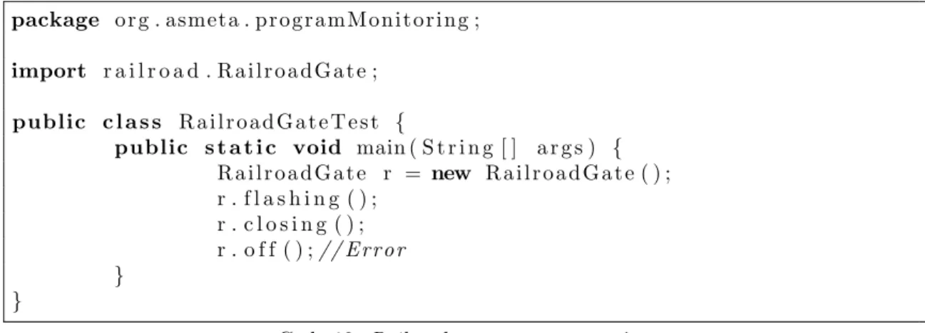
In code 12, instead, the calling sequence is not correct because the light is switched off while the gate is closing.

package o r g . asmeta . p r o g r a m M o n i t o r i n g ;

import r a i l r o a d . R a i l r o a d G a t e ;

public c l a s s R a i l r o a d G a t e T e s t {

public s t a t i c void main ( S t r i n g [ ] a r g s ) {

R a i l r o a d G a t e r = new R a i l r o a d G a t e ( ) ; r . f l a s h i n g ( ) ; r . c l o s i n g ( ) ; r . o f f ( ) ;// E r r o r } }

Code 12: Railroad gate wrong execution

We can see that, after executing the method closing(), the gate is CLOSING with the light FLASH; there is just one next ASM state compliant with the Java state and so the program can continue. After executing theoff()method, instead, the program monitor is not able to find any next ASM state compliant with the Java state. Indeed the Java state obtained after the execution of the method is{gate=CLOSIN G, light =OF F}, whereas the possible next ASM states are

{gate=CLOSIN G, light=F LASH}and{gate=CLOSED, light=F LASH}. See table 2 for the complete description.

Method call Java state Possible next ASM states

(in red the conformant state)

r.flashing(); gate = GateState.OPENED, light = LightState.FLASH

{gate = OPENED, light = OFF}, {gate = OPENED, light = FLASH} r.closing(); gate = GateState.CLOSING,

light = LightState.FLASH

{gate = OPENED, light = FLASH}, {gate = CLOSING, light = FLASH}

r.off(); gate = GateState.CLOSING,

light = LightState.OFF

{gate = CLOSING, light = FLASH},

{gate = CLOSED, light = FLASH}

Table 2: Railroad gate - Java and ASM execution

In code 13 the classRailroadGateSmart is shown, a more secure solution for the railroad gate problem. The class contains just one change method, the methodexec which accepts as input a variable of typeCommand, an enumerative that identifies the signals that the class can receive in order to modify its state. Depending on the command received and the current state, the method execexecutes the command if it is permitted in the state, otherwise it ignores it.

package r a i l r o a d ;

import o r g . asmeta . m o n i t o r i n g . Asm ;

import o r g . asmeta . m o n i t o r i n g . RunStep ;

import o r g . asmeta . m o n i t o r i n g . S t a r t M o n i t o r i n g ; @Asm( a s m F i l e = ” models / r a i l r o a d G a t e . asm” )

public c l a s s R a i l r o a d G a t e S m a r t { @FieldToFunction ( f u n c = ” l i g h t ” ) public L i g h t S t a t e l i g h t ; @FieldToFunction ( f u n c = ” g a t e ” ) public G a t e S t a t e g a t e ; @ S t a r t M o n i t o r i n g public R a i l r o a d G a t e S m a r t ( ) { l i g h t = L i g h t S t a t e . OFF ; g a t e = G a t e S t a t e .OPENED; } @RunStep

public void e x e c (Command command ) {

switch( command ) { case FLASH : l i g h t = L i g h t S t a t e . FLASH ; break; case OFF : i f( g a t e == G a t e S t a t e .OPENED) { l i g h t = L i g h t S t a t e . OFF ; } break; case CLOSED: i f( g a t e == G a t e S t a t e . CLOSING | | g a t e == G a t e S t a t e .CLOSED) { g a t e = G a t e S t a t e .CLOSED; } break; case OPENED: i f( g a t e == G a t e S t a t e .OPENING | | g a t e == G a t e S t a t e .OPENED) { g a t e = G a t e S t a t e .OPENED; } break; case CLOSING : i f( l i g h t == L i g h t S t a t e . FLASH && ( g a t e == G a t e S t a t e .OPENED | |g a t e == G a t e S t a t e . CLOSING ) ) { g a t e = G a t e S t a t e . CLOSING ; } break; case OPENING: i f( g a t e == G a t e S t a t e .CLOSED | | g a t e == G a t e S t a t e .OPENING) { g a t e = G a t e S t a t e .OPENING; } break; } } }

Code 13: Railroad gate smart Java code

shown in code 9, in this case any calling sequence is permitted7_{. We can run the Java code with}

any sequence of commands; the Java execution will be always compliant with the ASM simulation because if there is a valid command the Java code reacts in a correct way, and if there is a non correct command the Java code does not change its state. As we have previously seen, if the Java program moves to a valid state also the ASM machine can move to a valid state; if the Java program does not change its state (because it has received a wrong command), also the ASM machine can keep the state unchanged8_.

6.4

Monitoring an internally deterministic Java code with a

non-deterministic ASM model

Let’s see how it is possible to monitor an internally deterministic Java code with a non-deterministic ASM machine. We will see, as an example, theKnight’s Tour problem [16].

6.4.1 Knight’s tour

A knight is placed on the empty board; moving according to the rules of chess, it must reach each square of the board just once. The tour is closed if the last square visited by the knight is the square from which it began, otherwise isopen (our model looks for open tours).

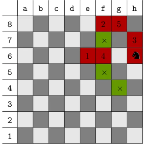
Table 3 shows in green the squares of the board that can be reached by the knight placed inh6.

a b c d e f g h 8 2 5 7 × 3 6 1 4 5 × 4 × 3 2 1

Table 3: Possible moves of knight placed inh6

We can see that the knight has started his tour ine6and, after 5 moves, he has arrived in h6 (e6 - f8 - h7 - f6 - g8 - h6). From there he can go inf7,f5or g4, but not ing8, because he has already visited it.

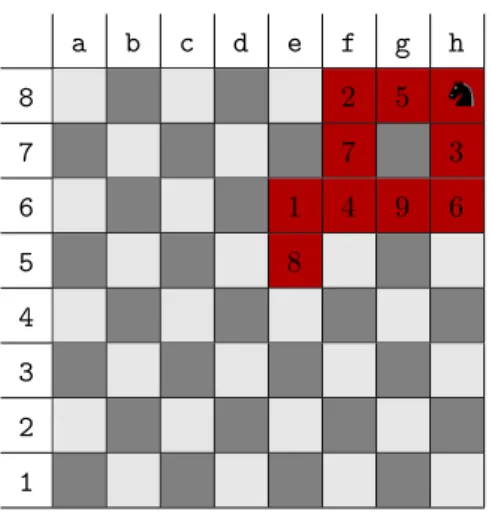
It is possible that a tour, nevertheless there are squares not yet visited, can not be completed because the knight is blocked in a square from which it can not execute any valid move. Table 4 shows a tour that can not be completed; the knight has continued the tour shown in table 3 with 4 more moves (h6-f7-e5-g6-h8) arriving inh8: from there he can not execute any valid move because all the squares that are reachable with theknight move (f7and g6) have already been visited.

Let’s see the formal specification of the problem in code 14.

asm KnightTour

7_{A sequence of method calls is also identified by the current values of the method parameters. For this reason}

we can talk of different sequences of call methods also in this example in which there is just one method.

a b c d e f g h 8 2 5 7 7 3 6 1 4 9 6 5 8 4 3 2 1

Table 4: Knight blocked inh8

import . . / . . / . . / . . / . . / asm examples /STDL/ S t a n d a r d L i b r a r y

signature:

enum domain S t a t u s = {VISITED | EMPTY}

domain Rows subsetof I n t e g e r

domain Columns subsetof I n t e g e r

dynamic c on t ro ll e d posX : Rows

dynamic c on t ro ll e d posY : Columns

dynamic monitored i n i t X : Rows

dynamic monitored i n i t Y : Columns

dynamic c on t ro ll e d board : Prod ( Rows , Columns ) −> S t a t u s

d e f i n i t i o n s:

domain Rows = {0 . . 7} domain Columns = {0 . . 7}

main rule r Main =

choose $x in Rows , $y in Columns with

board ( $x , $y ) = EMPTY and

( ( abs ( posX − $x ) = 1 and abs ( posY − $y ) = 2 ) o r ( abs ( posX − $x ) = 2 and abs ( posY − $y ) = 1 ) ) do par posX := $x posY := $y board ( $x , $y ) := VISITED endpar d e f a u l t i n i t s 0 : function posX = i n i t X function posY = i n i t Y

function board ( $x in Rows , $y in Columns ) =

i f ( $x = i n i t X and $y = i n i t Y ) then

VISITED

e l s e

EMPTY

Code 14: Knight’s tour ASM model

The ASM model, at each step, chooses non-deterministically a square of the board between those that are associated with a legal move and marks it asVISITED. The ASM model stops its execution when the update set is empty, that is when it can not find any legal move; a legal move can not be find because the knight is blocked or because he has finished the tour.

In code 15 we can see a non-deterministic Java code. The non-determinism isinternal because the behavior of the methodexecMove() is non-deterministic.

package k n i g h t T o u r ;

import j a v a . u t i l . A r r a y L i s t ;

import j a v a . u t i l . Random ;

import o r g . asmeta . m o n i t o r i n g . Asm ;

import o r g . asmeta . m o n i t o r i n g . F i e l d T o F u n c t i o n ;

import o r g . asmeta . m o n i t o r i n g . I n i t ;

import o r g . asmeta . m o n i t o r i n g . RunStep ;

import o r g . asmeta . m o n i t o r i n g . S t a r t M o n i t o r i n g ;

@Asm( a s m F i l e = ” models / nonDetModels / KnightTour . asm” )

public c l a s s KnightTour { @FieldToFunction ( f u n c = ” posX ” ) public i n t x ; @FieldToFunction ( f u n c = ” posY ” ) public i n t y ; private S t a t u s [ ] [ ] board ; @ S t a r t M o n i t o r i n g public KnightTour ( @ I n i t ( f u n c = ” i n i t X ” , a r g s = { }) i n t x , @ I n i t ( f u n c = ” i n i t Y ” , a r g s = { }) i n t y ) { t h i s. x = x ; t h i s. y = y ; board = new S t a t u s [ 8 ] [ 8 ] ; f o r(i n t i = 0 ; i < board . l e n g t h ; i ++) { f o r(i n t j = 0 ; j < board [ i ] . l e n g t h ; j ++) { board [ i ] [ j ] = S t a t u s .EMPTY; } } board [ x ] [ y ] = S t a t u s . VISITED ; } public void f i n d T o u r ( ) { while( execMove ( ) ) ; } @RunStep

private boolean execMove ( ) {

A r r a y L i s t<i n t[ ]> p o s s i b l e C h o i c e s = g e t P o s s i b l e M o v e s ( ) ;

i n t numOfMoves = p o s s i b l e C h o i c e s . s i z e ( ) ;

i f( numOfMoves > 0 ) {

i n t[ ] c h o i c e = p o s s i b l e C h o i c e s . g e t (

x = c h o i c e [ 0 ] ; y = c h o i c e [ 1 ] ; board [ x ] [ y ] = S t a t u s . VISITED ; return true; } return f a l s e; }

private boolean a v a i l a b l e M o v e (i n t newX , i n t newY ) {

return ( ( newX >= 0 && newX < 8 ) && ( newY >= 0 && newY < 8 ) ) && board [ newX ] [ newY]== S t a t u s .EMPTY;

} private A r r a y L i s t<i n t[ ]> g e t P o s s i b l e M o v e s ( ) { A r r a y L i s t<i n t[ ]> p o s s i b l e C h o i c e s = new A r r a y L i s t<i n t[ ]>( ) ; i n t[ ] c h o i c e = new i n t[ 2 ] ; c h o i c e [ 0 ] = x + 1 ; c h o i c e [ 1 ] = y + 2 ; i f ( a v a i l a b l e M o v e ( c h o i c e [ 0 ] , c h o i c e [ 1 ] ) ) { p o s s i b l e C h o i c e s . add ( c h o i c e . c l o n e ( ) ) ; } c h o i c e [ 1 ] = y − 2 ; i f ( a v a i l a b l e M o v e ( c h o i c e [ 0 ] , c h o i c e [ 1 ] ) ) { p o s s i b l e C h o i c e s . add ( c h o i c e . c l o n e ( ) ) ; } c h o i c e [ 0 ] = x − 1 ; i f ( a v a i l a b l e M o v e ( c h o i c e [ 0 ] , c h o i c e [ 1 ] ) ) { p o s s i b l e C h o i c e s . add ( c h o i c e . c l o n e ( ) ) ; } c h o i c e [ 1 ] = y + 2 ; i f ( a v a i l a b l e M o v e ( c h o i c e [ 0 ] , c h o i c e [ 1 ] ) ) { p o s s i b l e C h o i c e s . add ( c h o i c e . c l o n e ( ) ) ; } c h o i c e [ 0 ] = x − 2 ; c h o i c e [ 1 ] = y − 1 ; i f ( a v a i l a b l e M o v e ( c h o i c e [ 0 ] , c h o i c e [ 1 ] ) ) { p o s s i b l e C h o i c e s . add ( c h o i c e . c l o n e ( ) ) ; } c h o i c e [ 0 ] = x + 2 ; i f ( a v a i l a b l e M o v e ( c h o i c e [ 0 ] , c h o i c e [ 1 ] ) ) { p o s s i b l e C h o i c e s . add ( c h o i c e . c l o n e ( ) ) ; } c h o i c e [ 1 ] = y + 1 ; i f ( a v a i l a b l e M o v e ( c h o i c e [ 0 ] , c h o i c e [ 1 ] ) ) { p o s s i b l e C h o i c e s . add ( c h o i c e . c l o n e ( ) ) ; } c h o i c e [ 0 ] = x − 2 ; i f ( a v a i l a b l e M o v e ( c h o i c e [ 0 ] , c h o i c e [ 1 ] ) ) { p o s s i b l e C h o i c e s . add ( c h o i c e . c l o n e ( ) ) ; } return p o s s i b l e C h o i c e s ; }

private enum S t a t u s {

VISITED , EMPTY;

} }

Code 15: Knight’s tour Java code

As the ASM model, also the Java code chooses non-deterministically one move between those valid (let’s see the change methodexecMove()).

Deterministic version of the knight’s tour problem As we have seen in section 6.2 it is possible that the Java code is deterministic, nevertheless the corresponding ASM model is non-deterministic. Code 16 shows a modified version of code 15, in which a resolution strategy is implemented9_{. The code chooses, between the legal moves, the move which gets the knight closer}

to the middle of the board. We can notice that the Java code isfully deterministic:

• internally deterministic: the bodies of the methods do not contain any non-deterministic statements;

• externally deterministic: there is only one change methodfindTour(), that is the user of the class can interact with the object in just one way. So, we do not have to monitor the way the object is used.

The corresponding ASM model is the same as before. So, if the Java code is compliant, the Java run (given an initial state there is just one run) corresponds to one of the several ASM runs.

package k n i g h t T o u r ;

import j a v a . u t i l . A r r a y L i s t ;

import j a v a . u t i l . C o l l e c t i o n s ;

import o r g . asmeta . m o n i t o r i n g . Asm ;

import o r g . asmeta . m o n i t o r i n g . F i e l d T o F u n c t i o n ;

import o r g . asmeta . m o n i t o r i n g . I n i t ;

import o r g . asmeta . m o n i t o r i n g . RunStep ;

import o r g . asmeta . m o n i t o r i n g . S t a r t M o n i t o r i n g ;

@Asm( a s m F i l e = ” models / nonDetModels / KnightTour . asm” )

public c l a s s K n i g h t T o u r M i d d l e S t r a t e g y { @FieldToFunction ( f u n c = ” posX ” ) public i n t x ; @FieldToFunction ( f u n c = ” posY ” ) public i n t y ; private S t a t u s [ ] [ ] board ; @ S t a r t M o n i t o r i n g public K n i g h t T o u r M i d d l e S t r a t e g y ( @ I n i t ( f u n c = ” i n i t X ” , a r g s = { }) i n t x , @ I n i t ( f u n c = ” i n i t Y ” , a r g s = { }) i n t y ) { t h i s. x = x ; t h i s. y = y ; board = new S t a t u s [ 8 ] [ 8 ] ; f o r(i n t i = 0 ; i < board . l e n g t h ; i ++) { f o r(i n t j = 0 ; j < board [ i ] . l e n g t h ; j ++) { 9_{This code never reaches a complete tour from any initial state.}

board [ i ] [ j ] = S t a t u s .EMPTY; } } board [ x ] [ y ] = S t a t u s . VISITED ; } public void f i n d T o u r ( ) { while( execMove ( ) ) ; } @RunStep

private boolean execMove ( ) {

A r r a y L i s t<Square> p o s s i b l e C h o i c e s = g e t P o s s i b l e M o v e s ( ) ; i n t numOfMoves = p o s s i b l e C h o i c e s . s i z e ( ) ; i f( numOfMoves > 0 ) { C o l l e c t i o n s . s o r t ( p o s s i b l e C h o i c e s ) ; S q u a r e c h o i c e = p o s s i b l e C h o i c e s . g e t ( 0 ) ; x = c h o i c e . x ; y = c h o i c e . y ; board [ x ] [ y ] = S t a t u s . VISITED ; return true; } return f a l s e; }

private boolean a v a i l a b l e M o v e (i n t newX , i n t newY ) {

return ( ( newX >= 0 && newX < 8 ) && ( newY >= 0 && newY < 8 ) ) && board [ newX ] [ newY]== S t a t u s .EMPTY;

}

private A r r a y L i s t<Square> g e t P o s s i b l e M o v e s ( ) {

A r r a y L i s t<Square> p o s s i b l e C h o i c e s = new A r r a y L i s t<Square>( ) ;

i n t tempX = x + 1 ;

i n t tempY = y + 2 ;

i f ( a v a i l a b l e M o v e ( tempX , tempY ) ) {

p o s s i b l e C h o i c e s . add (new S q u a r e ( tempX , tempY ) ) ;

}

tempY = y − 2 ;

i f ( a v a i l a b l e M o v e ( tempX , tempY ) ) {

p o s s i b l e C h o i c e s . add (new S q u a r e ( tempX , tempY ) ) ;

}

tempX = x − 1 ;

i f ( a v a i l a b l e M o v e ( tempX , tempY ) ) {

p o s s i b l e C h o i c e s . add (new S q u a r e ( tempX , tempY ) ) ;

}

tempY = y + 2 ;

i f ( a v a i l a b l e M o v e ( tempX , tempY ) ) {

p o s s i b l e C h o i c e s . add (new S q u a r e ( tempX , tempY ) ) ;

}

tempX = x − 2 ; tempY = y − 1 ;

i f ( a v a i l a b l e M o v e ( tempX , tempY ) ) {

}

tempX = x + 2 ;

i f ( a v a i l a b l e M o v e ( tempX , tempY ) ) {

p o s s i b l e C h o i c e s . add (new S q u a r e ( tempX , tempY ) ) ;

}

tempY = y + 1 ;

i f ( a v a i l a b l e M o v e ( tempX , tempY ) ) {

p o s s i b l e C h o i c e s . add (new S q u a r e ( tempX , tempY ) ) ;

}

tempX = x − 2 ;

i f ( a v a i l a b l e M o v e ( tempX , tempY ) ) {

p o s s i b l e C h o i c e s . add (new S q u a r e ( tempX , tempY ) ) ;

} return p o s s i b l e C h o i c e s ; } private enum S t a t u s { VISITED , EMPTY; } }

c l a s s S q u a r e implements Comparable<Square> { i n t x ; i n t y ; public S q u a r e (i n t x , i n t y ) { t h i s. x = x ; t h i s. y = y ; } @Override public i n t compareTo ( S q u a r e o ) {

double t h i s D i s t a n c e F r o m M i d d l e = Math . pow ( x − 3 . 5 , 2 ) + Math . pow ( y − 3 . 5 , 2 ) ;

double oDistanceFromMiddle = Math . pow ( o . x − 3 . 5 , 2 ) +

Math . pow ( o . y − 3 . 5 , 2 ) ; i f( t h i s D i s t a n c e F r o m M i d d l e > oDistanceFromMiddle ) { return 1 ; } e l s e i f( t h i s D i s t a n c e F r o m M i d d l e == oDistanceFromMiddle ) { return 0 ; } e l s e { return −1; } } }