Digital Commons @ Trinity
Computer Science Honors Theses
Computer Science Department
5-2019
Short Term Load Forecasting Using Recurrent and
Feedforward Neural Networks
Andrew K. Loder
Trinity University, [email protected]
Follow this and additional works at:
https://digitalcommons.trinity.edu/compsci_honors
This Thesis open access is brought to you for free and open access by the Computer Science Department at Digital Commons @ Trinity. It has been accepted for inclusion in Computer Science Honors Theses by an authorized administrator of Digital Commons @ Trinity. For more information, please [email protected].
Recommended Citation
Loder, Andrew K., "Short Term Load Forecasting Using Recurrent and Feedforward Neural Networks" (2019).Computer Science Honors Theses. 46.
Short Term Load Forecasting Using Recurrent and
Feedforward Neural Networks
Andrew Loder
Abstract
Accurate load forecasting greatly influences energy production planning. If the demand forecast is inaccurate this could lead to blackouts or waste of precious energy. This paper compares many innovative networks on the basis of accuracy. The first is a feedforward neural network (FFNN). Next we look at different models of Recurrent Neural Networks (RNN) specifically long short term Memory (LSTM). Finally we explore combining the two approaches into a hybrid network. We will be predicting load with an hourly granularity also known as short term load forecasting (STLF). We will be applying these approaches to real world data sets from www.eia.govover a period of about 4 years. Our approach will focus on the integration of historical time features from the last hour, day, month, etc. with the inclusion of RNN methods. We show that the included time features reduce the overall error and increase generalizability. We combine this with features such as weather, cyclical time features, cloud cover, and the day of the year to further reduce the error. We will then compare the approaches to reveal that the correct handling of time features significantly improves the model by learning hidden features.
I would like to thank my thesis advisor Dr. Lewis for his continued support and guidance over the course of this thesis as well as my time at Trinity. He was one of my first teachers at Trinity and now he is one of my last.
Thank you to my brother who has inspired this thesis and given me guidance throughout the process.
I would also like to thank Amulya Deva for editing this thesis and making sure that my grammar is, for the most part, in check.
Short Term Load Forecasting Using Recurrent and Feedforward Neural Networks
Andrew Loder
A departmental senior thesis submitted to the Department of Computer Science at Trinity University in partial fulfillment of the requirements for graduation
with departmental honors. April 22, 2019
Thesis Advisor Department Chair
Associate Vice President for
Academic Affairs
Student Copyright Declaration: the author has selected the following copyright provision:
[X] This thesis is licensed under the Creative Commons Attribution-NonCommercial-NoDerivs Li-cense, which allows some noncommercial copying and distribution of the thesis, given proper attri-bution. To view a copy of this license, visit http://creativecommons.org/licenses/ or send a letter to Creative Commons, 559 Nathan Abbott Way, Stanford, California 94305, USA.
[ ] This thesis is protected under the provisions of U.S. Code Title 17. Any copying of this work other than “fair use” (17 USC 107) is prohibited without the copyright holder’s permission. [ ] Other:
Distribution options for digital thesis:
[X] Open Access (full-text discoverable via search engines)
[ ] Restricted to campus viewing only (allow access only on the Trinity University campus via
Using Recurrent and Feedforward
Neural Networks
Contents
1 Introduction 1
1.1 Introduction . . . 1
2 Background Knowledge 2 2.1 Developments in Machine Learning . . . 2
2.2 The Problem: Energy Load Balancing . . . 3
2.3 Data Driven and Simulation Approaches . . . 5
2.3.1 Data Driven Models . . . 5
2.4 Neural Network Background Knowledge . . . 6
2.4.1 Feedforward neural Networks . . . 7
2.4.2 Training . . . 7
2.4.3 Recurrent Neural Network . . . 9
2.5 Dropout Layer . . . 10
2.6 Previous Approaches . . . 10
3 Approach 15 3.1 Introduction . . . 15
3.3.1 Temperature . . . 16
3.3.2 Historical . . . 18
3.3.3 User Behavior . . . 18
3.3.4 Cyclical Time Features . . . 19
3.4 Data Integrity . . . 19 3.5 Approach . . . 21 3.6 FFNN Model . . . 22 3.7 LSTM Model . . . 22 3.8 Hybrid Model . . . 25 4 Results 27 4.1 Overall . . . 27 4.2 Comparison . . . 28 4.2.1 Spring . . . 28 4.2.2 Summer . . . 30 4.2.3 Fall . . . 30 4.2.4 Winter . . . 31 4.2.5 Overall Error . . . 33 4.3 FFNN . . . 33 4.4 LSTM . . . 35 4.5 Hybrid . . . 35 4.5.1 Activation Functions . . . 35 4.5.2 Sequence Size . . . 36 5 Conclusion 37
List of Tables
3.1 Features for the FFNN. . . 23
3.2 Features for the LSTM Model. . . 24
3.3 Features for the Hybrid Model. . . 26
4.1 The errors of the test set for a given model . . . 28
4.2 The errors of the test set for a given model . . . 33
4.3 Size of hidden layer and error. . . 34
4.4 Comparison of the tanh and ReLU error . . . 36
2.1 The Balancing Areas for the United States Source: U.S. Energy Information
Administration. . . 4
2.2 A simple Neuron. . . 6
2.3 Feedforward Neural Network with 3 hidden layers. . . 8
2.4 Gradient Decent where z axis is error, y and x axis are weights. Source: Wikipedia. . . 8
2.5 A recurrent neuron and the unfolding. . . 9
2.6 Long Short Term Memory cell unfolded. . . 12
3.1 2017-05-09 Temperature . . . 17
3.2 Time feature Encoded with sin and cos. . . 20
3.3 Feedforward Neural Network Structure. . . 23
3.4 Long Short Term Memory Network Structure. . . 24
3.5 Hybrid Network Structure. . . 25
4.1 Prediction comparison graph for spring. . . 29
4.2 Prediction comparison graph for average day summer. . . 30
4.4 Prediction comparison graph for winter. . . 32 4.5 Feedforward Neural Network Layer Training Comparison. . . 34 4.6 Not training correctly. . . 35
Introduction
1.1
Introduction
This paper is designed to walk through our approach to this problem in four steps. First we will reveal the necessary background knowledge so that one becomes acquainted with the problem and how we are attempting to solve this problem. We will start with the history of artificial intelligence. We then will introduce the problem along with the necessary background knowledge to fully understand it. We then take a look at other approaches that have seen real world implementations. Next, we introduce the background knowledge of our proposed solution to the problem, beginning with neural networks. We then pull from recent academic literature on this subject to further build our approach. After all of this background analysis has been done we finally detail our approach which consists of threefold, an FFNN, LSTM, and a hybrid approach. Lastly, we detail and conclude our findings.
Chapter 2
Background Knowledge
2.1
Developments in Machine Learning
To begin we must understand some historical context regarding the field of machine learning. Neural networks has been around since the 1950s and extensive research has been conducted ever since. Research into neural networks have been exploding in recent years. This is mostly due to recent development in deep neural networks. These developments allow for great improvements in computer vision, natural language processing, and speech recognition. The field before deep learning was mostly fixed on single layer neural networks with hand-designed features. It is provable that deep neural networks outperform single layer neural networks in terms of learning and accuracy.
The rise of cheap storage and big data sets are other contributing factors to the preva-lence of neural network research. The more data one feeds into a neural network, the more the network can adjust to consider that data point and allow it to generalize [5]. As we expand our resources to collect more data we can further the intelligence of our systems. We can see this in the coming years with the adoption of smart grids which will gather data
from the consumer’s electric meter.
Access to computational resources to run larger models have greatly improved the results we can achieve. The more neurons we can have in the model the more complex we can make the fit. Compared to a human brain, modern day neural networks are still an order of magnitude smaller [5]. While modern day artificial neurons do not represent neurons in a brain, this comparison gives the reader an idea of the relative computational capacity of these entities.
2.2
The Problem: Energy Load Balancing
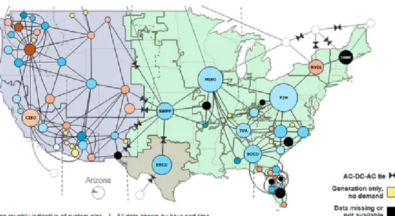
The problem we will be addressing is training a deep neural network to predict the hourly energy load of a given load balancing area. A load balancing area is governed by a load balancing authority that ensures that power system demand and supply are finely balanced. The load balancing areas for the United States are seen in Figure 2.1 as the small dots. The balance is needed for safety, cost saving, and reliability. These load balancing authorities ensure that there are no blackouts if the supply is too low, and aim to minimize waste if the supply is too high. They may also trade with neighboring load balancing authorities to further ensure that energy is in balance. In this paper we are not concerned with the supply side of this equation, rather, we are concerned with the demand of a given area. We chose a load balancing area because they put out hourly information about load demand and other data-points on www.eia.gov.
We will be focusing on the balancing area known as Tucson Electrical Power Company (TEPC) shown as the peach dot in the very bottom left of Figure 2.1 in Arizona nearest to New Mexico. We chose this for three reasons. First, it is a small load balancing area containing one major city, Tuscon. The localization allows us to only have to consider one
4
Figure 2.1: The Balancing Areas for the United States Source: U.S. Energy Information Administration.
weather station, the Tucson International Airport. This further increases the accuracy of the weather for the whole of the load balancing area which factors into the temperature variable in our model. Second, TEPC has not changed its service area drastically within the time period of the data we will be considering. It is important to consider how this data set has changed over time. Load balancing areas are not static entities, they may change their service area from time to time. Third, the TEPC region has relatively constant weather conditions. Weather is hard to predict due to its complexity, for example, the influence of cloud systems. The theory is that Tuscon does not receive too many cloud systems or unique weather conditions such as hurricanes. Therefore there will be fewer anomalies in the data set allowing for the model to generate a better fit.
2.3
Data Driven and Simulation Approaches
There are two types of models that are prevalent in this space, simulation models and data driven models. Simulation models use thermodynamics to estimate and analyze energy consumption. These can only be applied to physical traits of buildings and the knowledge of the environment that the buildings occupy.
Data driven models rely on historical data to estimate energy consumption. This model is compelling to most because of the new spring of artificial intelligence techniques and the widespread availability of data. Another appealing trait of data driven models is their automated nature. Once a model has been created for one grid, we can train and apply that model on another grid. This is in direct contrast to simulation models since simulation models require more labor to apply it to other buildings.
2.3.1 Data Driven Models
Within data driven models there are two active research areas in load forecasting: short term load forecasting (STLF) and long term load forecasting (LTLF). STLF, the area we are focusing on, is the forecasting of energy demand from several minutes up to one week in the future. LTLF is focused on predicting the future load with the forecast period of a year and above. There are vastly different problems when implementing an STLF versus an LTLF. The problem with STLF is reducing the jitter of a given prediction. The problem with LTLF is that there are not accurate weather reports for its given forecast period, and weather is the biggest driving factor in load demand.
STLF is used by the load balancing authorities to generate a day look-ahead to ensure that the grid has time to react to demand changes. If the outlook is inaccurate, it can lead to power loss due to underestimation and on the other end, it can lead to electricity waste
6
due to overestimation. LTLF is used in the same way. It is used to see if utility companies need to build additional infrastructure to keep up with demand.
2.4
Neural Network Background Knowledge
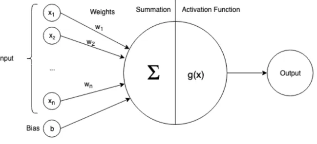
To understand the approaches to the problem we must first understand the basic concepts. The simplest unit of a neural network is a neuron, Figure 2.2. This neuron will consist of many inputs xi and weights wi which will be summed up to one value then fed into an
activation function that generates the output.
Figure 2.2: A simple Neuron.
An activation function is simply a function applied to the summation of inputs. There are many types of activation functions i.e. sigmoid, tanh, etc. The most popular and effective in recent research is the rectified linear unit (ReLU) [5]. This is defined by the
following equation. ReLU(x) = x ifx >0 0 ifx <= 0
2.4.1 Feedforward neural Networks
A Feedforward neural network (FFNN) is what a user with previous knowledge would perceive as a simple neural network. The prominent features are that data is only fed forward through the network and there are multiple hidden layers as illustrated in Figure 2.3. An FFNN contains 3 distinct layers. The input layer which feeds the data, also known as features, into the first hidden layer. A hidden layer contains neurons that receive the input from the previous layer and feed their output into the next layer. For the sake of this paper we will assume that every layer is densely connected, meaning a neuron connects to every other neuron in the adjacent layers. Lastly we have the output layer which outputs a single value for every neuron that exists in it. For a continuous prediction we will have one neuron in the output layer, but for other predictions such as categorical or to predict many continuous variables we would have multiple.
2.4.2 Training
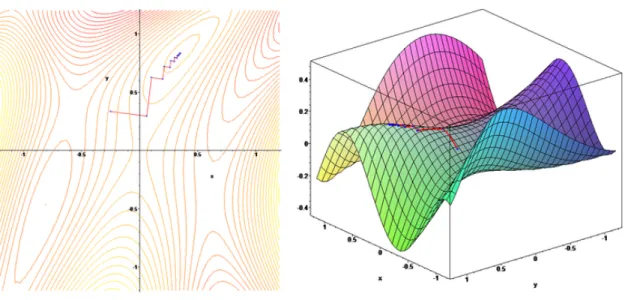
Training the network is the most important part of all. This is where the magic happens. Back-propagation allows for the information from the error of the output to flow backward through the network in order to compute the gradient. This gradient is the direction of the greatest decrease in error, see Figure 2.4. The mission of back-propagation is to find the global minima of the error plane by adjusting the weights of the layers where the error, on some level, is defined as how close the prediction is to the real value. To explain this in depth is outside of the scope of this introduction. In this paper we will be using Adam [9]
8
Figure 2.3: Feedforward Neural Network with 3 hidden layers.
and not delving into the world of training.
Figure 2.4: Gradient Decent where z axis is error, y and x axis are weights. Source: Wikipedia.
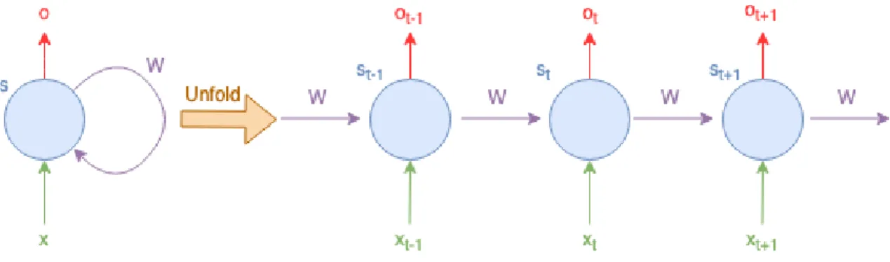
2.4.3 Recurrent Neural Network
A recurrent neural network (RNN) is one where the output of a neuron feeds into its input. We can explain this in much more simple terms. Lets say we have a problem where a document was damaged and some of the words were unreadable. As humans we would approach this problem by reading the document and making an educated guess that aligned with the context of the sentence and document. RNNs solve this problem similarly, they would take in the series of words to understand the context of the sentence, then predict the unreadable word. They do this through self-loops which allow the information to persist from the first to the last word. This structure can be confusing since we self reference, but one can unfold this recurrent network. Once we unfold one can think of it as many copied layers in a normal neural network passing an extra input into their successor as shown in Figure 2.5. There are many variations of an RNN, one of which, long short term memory (LSTM) we will describe later.
10
2.5
Dropout Layer
The simplest way of reducing overfitting is by adding a dropout layer to a model. A dropout layer randomly drops units along with their connections from a neural network during training [12]. This prevents units from relying on one another too much because during training one unit can not always rely on another unit being there. This allows units to reach a value that independently adds value to the prediction rather than relying on each other. The only parameter we will give to the dropout layer is the probability that a unit will be dropped. The original paper cited above finds that the best dropout probability is 30%. We will be using this probability as a starting point for all of our models.
2.6
Previous Approaches
There have been several approaches used in STLF: Autoregressive integrated moving av-erage (ARIMA), recurrent neural network (RNN), feedforward neural network (FFNN), extreme learning, and long short term memory (LSTM).
Din et al. compares the performance of a feedforward neural network and recurrent neural network [4]. They use the New England-ISO data set from 2007 to 2012. The features of this data-set include date, hour, electricity price, dry bulb, dew point, and system load. The features they decide to use are temperature effects, time effects, holiday effects, and lagged load.
They included temperature effects for two reasons. The first is when you have lower or higher temperature, the climate control system in buildings will consume energy to maintain a reasonable temperature. The second reason is humidity. Buildings will also control this factor as well. They address the time effects by adding two inputs, the hour and the weekday. This is particularly interesting due to the lack of yearly data. The holiday effects are simple
- if it is a workday or not. Workdays and non-workdays have different energy consumption profiles due to human actors changing their behavior. Lastly, they consider lagged load to contain vital information about specific patterns of energy consumption. They include previous week and previous day same hour load, and previous 24 hour average load. They also include data distribution effects over the past 24 hours. They use skewness, kurtosis, variance, and periodicity. They find that these features uncover hidden patterns hidden in the data-set. They conclude that weather, time, holidays, lagged load, and data distribution are found to be the most dominant factors. They also show that the RNN has less error than the FFNN on all domains and error calculations.
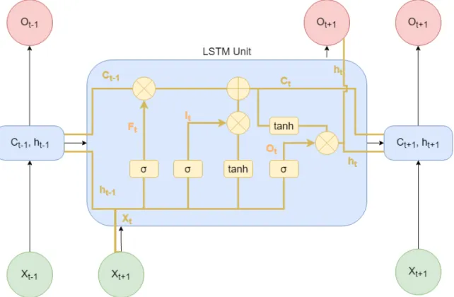
Liu et al. propose a long short term network (LSTM) based on an RNN for STLF [10]. LSTM’s are a type of RNN where some variables from one iteration are fed into the next as illustrated in Figure 2.6.
An LSTM unit is composed of an input gate(It), output gate (Ot), and a forget gate
(Ft). To further understand the figure, σ is an activation function, ct is the remembered
input, and ht is the previous output. The goal is to remember the previous input values
ct and forget some of the values using Ft and to factor the previous input into the output
we see at Ot. LSTMs were proposed to deal with the exploding and vanishing gradient
problems that were encountered with traditional RNNs [8]. An exploding gradient is a problem where the gradient, which is used to change the weights of the model, becomes too big and results in a numeric overflow. A vanishing gradient is one where the gradient gets too small, so much so that all training stops and the weights are not updated. This is the result of the chain rule when back propagating through the unfolded layers of an RNN.
One advantage they propose is that the RNN architecture introduces self-loops where they are able to produce paths that the gradient can flow for a long duration. This means that the model improves its accuracy at a constant rate. This property allows for the
12
model to neglect small local jitters which improves precision and generalizability. They acknowledge the downfall of RNNs, RNNs assume that all input variables are independent of each-other. In STLF and LTLF the previous value is not independent of the subsequent value so a traditional RNN is unsuitable for this task. In their conclusion they state that LSTMs can be used to forecast hour-ahead values with high precision.
Bouktif et al. focuses both on short term and monthly forecasting, proposing an LSTM-RNN [2]. They use a large data set from a metropolitan area from France covering a nine year period at a 30 minute resolution. They use a genetic algorithm to generate models with different time lag intervals, then pick the best lag time of the bunch. A genetic algorithm (GA) generates slight differences in the model, trains them, then picks the most accurate one, then repeats the process. GA works much like evolution. The GA allows for domain specific knowledge, like the amount of lagged load one should have, to be decoded and decided for you. They found that the LSTM-RNN had lower forecasting errors in the medium and short term when compared to the best machine learning algorithms.
Chen et al. finds that an ensemble strategy enhances the generalization capacity of the model [3]. Inspired by the ResNet architecture in [7], they propose a deep residual network. This architecture is used to force the network to preprocess related things before feeding it into the final network, like the temperature and load of a given hour then output that further into the model. During training they take snapshots of the model when the error is relatively low. Then they use those snapshots as an ensemble, meaning their outputs are averaged together when they are making a prediction. To simplify, they take neural networks that think a little bit differently and average their predictions. This leads to a more generalizable result because the weights of a snapshot are different allowing for more inputs to be considered since at each snapshot the impact of the input variables is different. There are several data-driven approaches to forecast LTLF. The biggest change between
14
the STLF and LTLF is the problem of exploding and vanishing gradients and the imprac-ticality of weather forecasts. These problems eliminate many of the techniques used for STLF and one of the biggest factors, weather, from the equation. We include these works because they take the same form of STLF models, forecasting with hourly granularity and encoding time features.
Agrawal et al. focused on generating a long term load forecasting using hourly pre-dictions [1]. They used the New England-ISO hourly data. They forewent weather data because it would require weather predictions for up to 5 years in the future. Errors in these forecasts were found to degrade the models performance. They found that the most important feature was the load demand for the same day and hour of the previous year.
They proposed a model of an RNN with LSTM cells. Due to exploding gradients, simple RNNs do not perform well on long term forecasts. LSTM cells allow for the RNN to remember long term dependencies and short term states. They also mention that FFNN assumes that the training and test data are independent. Since electricity load demand is a time series data - the assumption fails so FFNN is not suitable. Ultimately they find that LSTM-RNNs are suitable for forecasting with a mean absolute percentage error of 6.54. They concede that incorporating weather parameters into the data-set can be beneficial.
Approach
3.1
Introduction
3.2
Data
The data we will be using comes from two sources, the load data and the weather data. The load data for a given load balancing authority can be found atwww.eia.govand the weather data can be found at www.ncdc.noaa.gov. The weather station we will be using is from the Tucson International Airport in Arizona, network id GHCND:USW00023160. Load data from api.eia.gov/series/?api_key=BLANK&series_id=EBA.TEPC-ALL.D.H where one must sign up on the website and replace the API key with your own. This data and the corresponding code and data can also be found at https://github.com/aloder/ Senior-Thesis.
We will be using load and weather data from 2015-07-01 to 2018-06-30. A good amount of data points have been removed due to missing data or malformed data. In total there are 25,018 observations in the final data set as opposed to the total number of possible
16
observations, 26,304 meaning 1,286 (4%) observations have been removed. Further work should be done to clean the data more efficiently. It is important to note that missing data has a big impact on recurrent neural networks since we have to fill that missing data. We fill that missing data with the next available record, this is another error that could drastically affect the training and error rate.
3.3
Features
Feature selection is one of the most important steps in creating any machine learning model. A feature is an individual measurable property or characteristic of a phenomenon being observed [11]. Features are normally numeric but can be strings or other data types. For our purposes we will be encoding every string as a number either by using one hot encoding or by converting it to values using domain knowledge. One hot encoding is a tactic to represent variables that are linked but do not have an ordinal relationship [6]. We use one hot encoding to force the network to treat these values as independent.
3.3.1 Temperature
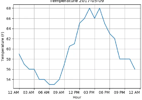
The two most important aspects of this problem is temperature and historical load. The biggest variable in energy consumption is temperature. This is due to climate control sys-tems like heating and air conditioning. Tuscon ranges from very hot during the day and very cool at night due to its climate. We can see this in Figure 3.1. These temperature fluctuations cause the heater to turn on when the temperatures are low and the air condi-tioning to turn on when the temperatures are high. The machine learning algorithm must learn this threshold and understand its correlation to achieve a lower error.
18
3.3.2 Historical
The second important aspect is historical features. The historical load and historical tem-perature can help the model identify trends in the data set [3]. For example comparing the last days temperature to this days temperature. If this days temperature is much hotter, one can assume that the load is going to be higher then the last days load. The network can use these measurements as further context to generate a correct prediction.
The problem with using historical features is that one needs to further condense the data set to support them. For instance, if we would like to have last months load fed into the prediction, one must fold the data set onto itself and remove a month from the entire data set, as we did. One must also interpret or drop the data points that are missing the last month field, further decreasing the size. This trade off is worthwhile since we have a big enough data set to train on and generate these historical data points as well.
3.3.3 User Behavior
Another important feature is user behavior. User behavior is how people interact and use energy in different scenarios. This aspect is one of the hardest ones to predict because there is no correct empirical way to rate user behavior besides their historical energy usage. This is one of the benefits about smart grids, they can better understand and account for individual buildings and users due to the granularity of their measurements. To somewhat account for user behavior we one hot encode whether it is a workday or not. One other thing we implemented was time features, such as hour of day and the day of year. This is included to help identify long term trends of a given hour or day.
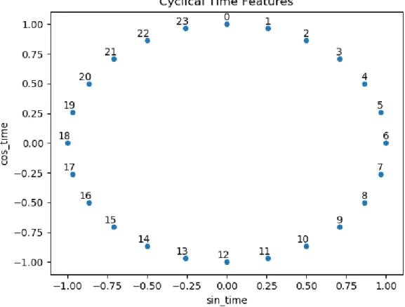
3.3.4 Cyclical Time Features
With time features, we encounter a problem. That problem is that time is cyclical but straight time features like hour or day of year are not. For example take hours of the day. There are 24 hours of the day so one would encode those hours using 0-23. The problem with this approach is that spatially 0 is the far away from 23 even though they are close to each-other, in regards to time.
To solve this problem we need to look at circles. We can transform a time feature into a circle using cosine and sine, see Figure 3.2. This allows for 23 to be right next to 0. The machine learning algorithm will be able to see the correlation which results in faster, more accurate fit. We apply this to day of year, day of week, and hour of day.
3.4
Data Integrity
A popular saying is trash in trash out. The trash in this case is the data. Some of the load data points are corrupted, and the question is how do we deal with that? The way we set up our models hurts us even more. We place a high value on historical load data but if that historical record does not exist, should we just throw out that data point? In time series data it is a little more difficult since we can not replace a missing data point with the average since the average depends on the time of day and other conditions. So our approach was to simply take the values around the corrupted data points and calculate the average between those values. This approach saves only a few of the data points but does improve model accuracy. Multiple predictions depend on the same data points since all predictions look at the same historical data points in all our models.
The biggest problem with this data set is its error. It is not easy to tell if energy usage of an hour just had a random spike in demand or if it was an error. The way we deal with
20
this is by setting a cap value where all the points above it are set to N/A, then we fill those N/As with the neighbor method above. This approach has worked well for our data set. The problem with this approach is consecutive missing data points. If there are consecutive missing data points we remove them from the record since repairing all of them is too labor intensive and will not greatly add to the accuracy of the model.
Another way we deal with this error is through manual observation. We have created a tool on processing to examine data points our model is having the most trouble predicting. If we deem it an error, we remove the points from the data set. This method is very inefficient because there is no empirical standard for dictating if a data point is an error or not. Leaving the user to use their expert knowledge, which has inherent bias since we know that the model is having trouble predicting this data point. We leave it to future work to devise a better system where to detect and replace errors in the data set.
3.5
Approach
Our approach will be threefold. We will look at the performance of three models FFNN, LSTM, and a hybrid model. The reasoning behind this is to see if the combination of the FFNN and the LSTM model will achieve better results since they both have drawbacks.
We used tensorflow v1.12.0 and trained the models on discrete GPU GTX 1080. We primarily used the tensorflow implementation of the Keras API to rapidly test different configurations of the models. We ran each model with a training set of 2016, 2017, and 2018 with the months of 2017 of 1,3,4,6,7,8. We tested the models on 2017 with the months of 2, 5, 9, and 11. We split the data set in such a way so that the model would be tested on each of the seasons all the while having enough training data to fit correctly. We also used a random validation split of 0.2 meaning 20% of the training set would be used to monitor
22
the training. We used the ADAM optimizer to train the model. We normalized the data using a min max scalar. We also tested normalizing using the z-score, but we found that the min max scalar worked better due to some of the variables not being in the form of a normal distribution. Over the course of the training we saved the model with the lowest error on the validation set. After the training is over we tested both the model that went through the entire training and the model that we saved. We then picked the model that performed the best on the testing set and saved their results. Over the course of the testing we found that the best model, determined by the validation set, always had the least error. After testing a model, we upload the results to tensorboard, a web based tool used to analyze results from tensorflow. In total we tested 65 different configurations of the proposed models.
3.6
FFNN Model
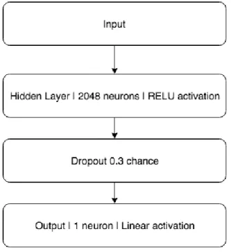
This model is a simple neural network that we found works best with four layers, see Figure 3.3. Through trial and error we found that using more then one dense hidden layer is unnecessary. We also found through trial and error that one of the best configurations is 2048 nodes with ReLU activation. We will detail this more in the results section. The features we use are detailed in Table 3.1.
3.7
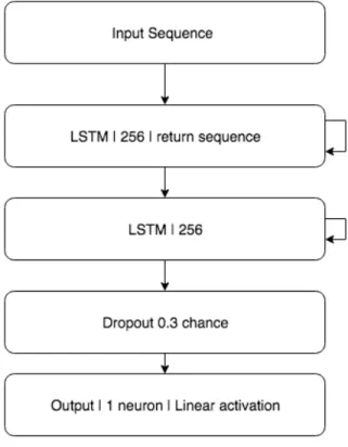
LSTM Model
This is a recurrent neural network implementation laid out in Figure 3.4. The difference is that we feed this network an array of features that are time stepped, and the time step we decided to use hourly. There is future work to be done on considering different time steps. Another consideration is the sequence size which is how many time steps do we want to
Figure 3.3: Feedforward Neural Network Structure.
Feature Note
Temperature (F) Year
Day of year Cyclical
Day of week (F) Cyclical
Time of day (hour) Cyclical
Past 24 hour mean load
Past 24 hour mean temperature Last Hour’s Load
Last Hour’s temperature
Cloud Cover Based on SKC in NOAA data set
Workday One hot encoded
24
include for each prediction. This can be hard to decide but with trial and error we can find the best time step to use [2]. In addition to the time step, we must also consider different features see Table 3.2.
Figure 3.4: Long Short Term Memory Network Structure.
Feature Note
Temperature (F)
Cloud Cover Based on SKC in NOAA data set
Load
Last Week Load Last Day Load
3.8
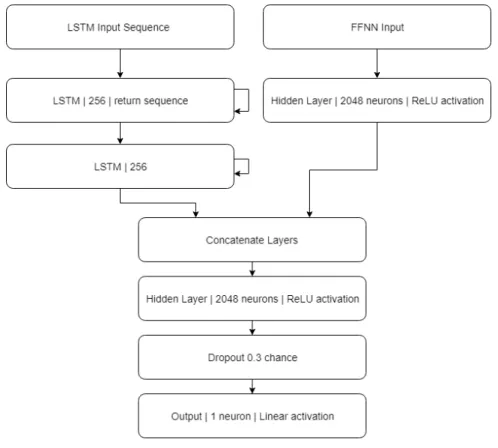
Hybrid Model
The hybrid model relies on the concatenation of the two models previously described. The idea behind this is to get the best traits of both models above. Our FFNN uses just a few historical data points, which is susceptible to errors since we depend on a small sample. LSTM takes in a series of historical data to predict the next data point. The problem with LSTM is that it can not take in the latest input since it can only rely on historical data. The FFNN takes in the most recent data and the LSTM handles the historical data Table 3.3. The layout of this hybrid model is more complicated then the previous models see Figure 3.5.
26
Feature Note Model
Temperature (F) Both
Cloud Cover Based on SKC in NOAA data set Both
Load LSTM
Last Week Load Both
Last Day Load Both
Workday One hot encoded FFNN
Day of week (F) Cyclical FFNN
Time of day (hour) Cyclical FFNN
Results
4.1
Overall
To gauge the results we use mean average percentage error (MAPE) because it is the easier to interpret when compared to, for example, root mean squared error (RMSE). As 4.1 shows FFNN is the model with the lowest percent error followed by the hybrid method, then LSTM. The FFNN performed very well for this situation given its unfavorable credibility in most academic literature. One would assume that the LSTM would have the best error. This could be due to the number of features that we choose for this given task since most research in the field of short term load forecasting with LSTMs only take into consideration the load data. The hybrid model performed in the middle landing a little bit closer to the FFNN than the LSTM network. This is most likely due to the hybrid network favoring the FFNN weights more than the LSTM network, but as we will show below the hybrid approach does beat the FFNN in some cases.
28
Model MAPE
FFNN 0.91
LSTM 1.22
Hybrid 0.95
Table 4.1: The errors of the test set for a given model
4.2
Comparison
To understand how well each model fit, we need to graph them for all four seasons since climate is one of the main causes of energy fluctuation. Each set of graphs is a selected day from the test dataset, meaning these data points were not used to train and the network has never seen these. First, we will explain the graph. The blue lines are the prediction and the orange lines are the actual values. Under the graphs is the error which shows us how off the model was at a given hour. We are going to be using a 24-hour marking scheme. These are in Universal Time and Tucson is in Mountain Standard Time.
4.2.1 Spring
We will first begin with spring as seen in Figure 4.1. As you can see in Figure 4.1 the FFNN has the best fit on the peak at midnight, the LSTM overestimates the peak, and the hybrid underestimated then over corrected. At around hour 15, we can see some models having trouble, with the top performer being the hybrid model. The increase to the peak was steady and no model shows any difficulty fitting to it.
This is due to the spring months being very cold at night, and in this case the low was 54 during the night.
30
4.2.2 Summer
We now look at prediction comparison for the typical summer day, see Figure 4.2. The sine like behavior of power consumption is very typical for the summer months. We can see that FFNN does the best by far almost mimicking the behavior almost exactly. Looking at the error graph we see the similarities of the LSTM and hybrid mistakes.
Figure 4.2: Prediction comparison graph for average day summer.
4.2.3 Fall
Next consider Figure 4.3. We can see that yet again the FFNN comes out with the best fit and the lowest error. The hybrid predictions resemble more of the FFNN predictions than the LSTM predictions. Further examination of the peaks reveals that the hybrid prediction
deviates from the FFNN prediction and resembles more of a flat peak that we see in the LSTM prediction which results in lower error.
Figure 4.3: Prediction comparison graph for a fall day.
4.2.4 Winter
Lastly let us consider a winter day shown in Figure 4.4. This day is particularly noisy which results in less smooth predictions from the models. We can see that the FFNN is the most smooth, followed by hybrid, then LSTM. The FFNN does the best at predicting between the two peaks, but the Hybrid network does the best at predicting the peaks.
32
4.2.5 Overall Error
To further understand how our models are performing given different circumstances we break down the results into seasons shown in Table 4.2. We used our test set with the following months as the seasons, February is winter, May is spring, September is summer, and November is fall. The FFNN performs considerably better in the summer, spring, and fall. The hybrid approach performs better in the winter. This can be due to the hybrid model unintentionally prioritizing winter fit or the LSTM combined with the FFNN reveals a hidden correlation.
Model Winter Spring Summer Fall
FFNN 1.15 0.88 0.83 0.81
LSTM 1.47 1.16 1.10 1.14
Hybrid 1.09 0.94 0.97 0.90
Table 4.2: The errors of the test set for a given model
4.3
FFNN
For the feedforward neural network we tested two factors to find the optimal network structure. First we tested the layer size, the results can be viewed in Table 4.3, and the training error can be viewed in Figure 4.5. We found that the best network structure comprised of a small number of layers an input layer, one hidden layer consisting of 2048 nodes, a dropout layer with a 0.3 chance and lastly a single node for the output layer. There is likely a marginally better network but through our testing, we did not find one. For future work, more conclusive testing must be done to ensure that more layers do not improve the results of the model.
34 Size MAPE 4096 0.96 2048 0.91 1024 0.98 512 0.97
Table 4.3: Size of hidden layer and error.
4.4
LSTM
We ran into problems with the implementation of the CuDNNLSTM on tensorflow. We found that the model would sometimes not be able to find the gradient and stagnate at an error rate. See Figure 4.6. By looking at the predictions we noticed a cap on the prediction value leaving plateaus on the lower and higher loads. This is probably put in place to combat the vanishing and exploding gradients that recurrent neural networks face. It is not clear how to fix this error, so we ignored the result and changed the model until it fits correctly.
Figure 4.6: Not training correctly.
4.5
Hybrid
4.5.1 Activation Functions
With this network we focused on testing the activation functions. The implementation of the CuDNNLSTM on tensorflow is fixed to the tanh activation function since they use some hardware tricks to make the training process faster on a GPU. We tested both tanh and ReLU on all layers with the ability to customize the activation function. We found that
36
ReLU performed better in both training time and MAPE as seen in Table 4.4.
Tanh ReLU
1.11 0.95
Table 4.4: Comparison of the tanh and ReLU error
4.5.2 Sequence Size
Using Bouktif et al. [2] as a guiding piece, we tested multiple sequence sizes under the same conditions to ensure that the best one was chosen as shown in Table 4.5. This shows us that there is an optimal sequence size and one can not keep increasing the sequence size expecting better results.
Sequence Size MAPE
3 1.01
6 0.95
12 2.61
Conclusion
This paper introduces three models for hour ahead energy forecasting, FFNN, LSTM, and Hybrid, then evaluates their accuracy. Contrary to our predispositions and many papers pre-dispositions we found that an FFNN with historical time features performed the marginally better then the hybrid network and significantly better then the LSTM network for pre-dicting the next hour load. In our review of academic literature on FFNN and LSTMs we have failed to find a paper that finds FFNNs performed better. This leads us to believe that this paper is unique in that regard.
We can point to several possible factors as to the poor performance of the proposed LSTM model. The most likely possibility is the importance of temperature in this data set. LSTMs are fed in a sequence of historical data, but not the most current data, leaving them at a disadvantage when compared to our proposed FFNN which has both the most important historical data as well as the current data. The second possibility is the very short term nature of our prediction. Most papers use LSTM architecture to predict longer than our time frame.
We finally propose a hybrid model. The intent was to combine the current data fed 37
38
into the FFNN and the historical data fed into the LSTM. Overall the hybrid approach did not perform better than the FFNN but in some circumstances, we show that the hybrid approach did perform better. To understand these results further, more research should be done on the proposed hybrid approach.
In conclusion, we find ourselves going against recent academic research that LSTMs perform the best compared to other approaches for short term load forecasting. Given the results we recommend the proposed FFNN for hour ahead load forecasting.
[1] Rahul Agrawal, Frankle Muchahary, and Madanmohan Tripathi. Long term load fore-casting with hourly predictions based on long-short-term-memory networks. pages 1–6, 02 2018.
[2] Salah Bouktif, Ali Fiaz, Ali Ouni, and Mohamed Adel Serhani. Optimal deep learning lstm model for electric load forecasting using feature selection and genetic algorithm: Comparison with machine learning approaches . Energies, 11(7), 2018.
[3] Kunjin Chen, Kunlong Chen, Qin Wang, Ziyu He, Jun Hu, and He Jinliang. Short-term load forecasting with deep residual networks. IEEE Transactions on Smart Grid, PP, 05 2018.
[4] G. M. U. Din and A. K. Marnerides. Short term power load forecasting using deep neural networks. In 2017 International Conference on Computing, Networking and Communications (ICNC), pages 594–598, Jan 2017.
[5] Ian Goodfellow, Yoshua Bengio, and Aaron Courville. Deep Learning. MIT Press, 2016. http://www.deeplearningbook.org.
[6] Cheng Guo and Felix Berkhahn. Entity embeddings of categorical variables. CoRR, abs/1604.06737, 2016.
40
[7] Kaiming He, Xiangyu Zhang, Shaoqing Ren, and Jian Sun. Deep residual learning for image recognition. 2016 IEEE Conference on Computer Vision and Pattern Recogni-tion (CVPR), pages 770–778, 2016.
[8] Sepp Hochreiter and Jrgen Schmidhuber. Long short-term memory. Neural computa-tion, 9:1735–80, 12 1997.
[9] Diederik P. Kingma and Jimmy Ba. Adam: A method for stochastic optimization, 2014.
[10] C. Liu, Z. Jin, J. Gu, and C. Qiu. Short-term load forecasting using a long short-term memory network. In2017 IEEE PES Innovative Smart Grid Technologies Conference Europe (ISGT-Europe), pages 1–6, Sep. 2017.
[11] John Maindonald. Pattern recognition and machine learning. Journal of Statistical Software, 17, 03 2007.
[12] Nitish Srivastava, Geoffrey Hinton, Alex Krizhevsky, Ilya Sutskever, and Ruslan Salakhutdinov. Dropout: a simple way to prevent neural networks from overfitting.