Techniques for Analyzing the Relationship between Population Density and Geographical Features of Interest

(1)

Procedia Environmental Sciences 27 ( 2015 ) 89 – 93

Peer-review under responsibility of Spatial Statistics 2015: Emerging Patterns committee doi: 10.1016/j.proenv.2015.07.116

ScienceDirect

Spatial Statistics 2015: Emerging Patterns

Techniques for analyzing the relationship between population

density and geographical features of interest

Amanda Johnson

a

, Colin Arrowsmith

b

*

a_{SAFEVIC, Murdoch Childrens Research Institue, Australia & Department of Paediatrics, Monash University, Australia} b_{RMIT University, School of Mathematical and Geospatial Sciences, 24 La Trobe Street, Melbourne, VIC 3000, Australia}

Abstract

This paper presents a study which explored a range of techniques for analysing the spatial relationship between population density and geographical features of interest at a global scale. Three categories of spatial analysis techniques were explored: traditional methods, spatial autocorrelation statistics and regression analysis. The correlation between the spatial distribution of Australian cinema screens and a global gridded population density dataset were used as the case study for the analysis.

Peer-review under responsibility of Spatial Statistics 2015: Emerging Patterns committee.

Keywords: spatial analysis; Moran’s I; Anselin’s I (LISA); global gridded dataset; regression analysis; cinema and screen studies

1. Introduction

This paper explores three categories of spatial analysis techniques which can be used at a global scale, to investigate the relationship between population density and the spatial distribution of a geographic feature of interest. The correlation between the spatial distribution of Australian cinema screens and a global gridded population density dataset were used as the case study. Category one is traditional analysis techniques and incorporates descriptive statistics and spatial distribution maps. Category two is spatial autocorrelation statistics and incorporates Moran’s Global I [1] and Anselin’s Local I [2]. The final category is regression analysis and

* Amanda Johnson. Tel.: +61 3 8341 6200; fax: +61 3 9348 1391.

E-mail address: [email protected]

(2)

incorporates ordinary least squares (OLS) regression and error residual testing using the global Moran’s I autocorrelation statistic.

2. Materials and Methods

2.1. Study Area

Australia is located in the Southern Hemisphere, between the South Pacific Ocean and the Indian Ocean, at latitudes of 10-45º S and longitudes of 113-153º E.

2.2. Data Collection

Two sources of data were used: cinema screens and population density. The cinema screen location dataset was a shapefile of point features, containing the longitude and latitude values of 501 Australian cinema screen addresses and the number of screens situated at each cinema (2,014 screens in total), as at the start of 2012. The details were obtained from a third party data collector as part of Australian Research Council (ARC) project DP120101940.

Population density data was sourced from the Socioeconomic Data and Applications Centre (SEDAC) at Columbia University. Three Year 2000 Gridded Population of the World version 3 (GPW v3) datasets with a spatial resolution of 2.5 arc-minute grid cells (~5 km² at the equator) were downloaded: Population Count Grid [3], Land and Geographic Unit Area Grids [4] and Population Density Grid [5].

A global gridded population density dataset was selected because they use spatial interpolation to transform native census data of varying resolutions into a consistent gridded format [6]. Therefore they have a spatial resolution which is consistent across nation boundaries, making them applicable for use in global scale studies.

2.3. Data Preparation

The four input datasets were transformed and spatially joined to create a shapefile of integer points, one for each gridded cell in the original SEDAC population density dataset. Attached to each point were six cell attribute values: number of cinema screens, land area in km², population count, population density per km², screen density per km² and screen density per person. The software used to prepare the data and subsequently conduct the spatial analysis was ArcGIS® and ArcMap™ by Esri.

3. Results

Please note: due publication space limitations, only 1 example for each spatial analysis category is presented below.

3.1. Traditional Spatial Analysis Tools

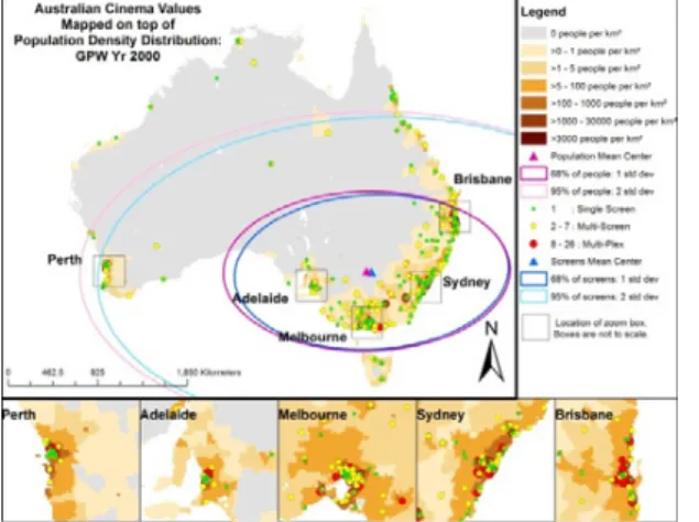
Figure 1 depicts the spatial distribution of Australian cinema screens as a graduated point pattern, mapped on top of the spatial density distribution of Australia’s population as a raster pattern. The one and two standard deviation ellipses and the geographic mean centres of the two datasets are also displayed, screens in blue, population in pink. When these datasets are mapped together there appears be a strong correlation between population density and cinema location. The dark brown more densely populated areas have multiple cinema points mapped on them, in particular the yellow multiscreen cinemas and red multiplex cinemas. Correspondingly, the lighter brown less populated areas of Australia have fewer cinema points mapped on them and they are they are often green one screen cinemas. The triangles representing the geographical mean center of the datasets are located in close proximately in the south-east corner of mainland Australia, as are the standard deviation ellipses.

(3)

3.2. Spatial Autocorrelation Statistics

Figure 2 maps the results of the Anselin local I spatial autocorrelation statistic using a distance threshold of 20 km and a CI of 95%, for the screens per km² and population per km² datasets. Positive spatial autocorrelation (clustering) was found to be present in both datasets, population density clusters are displayed in red and screen density clusters in purple. Cells found to be statistically non-significant are displayed in grey for the population density dataset and yellow for the screen density dataset. No outliers where found in the population density dataset but some were identified in the screen density dataset and are displayed as in pink and blue. The spatial distribution of the clustering varies between the two datasets. Screen density clusters are only found in the four largest metropolitan areas: Brisbane, Sydney, Melbourne and Perth. Population clusters are found in all of these areas but to a larger extent and are also present in Perth, Darwin, Tasmania and along the eastern seaboard.

Figure 1. Spatial distribution of Australian Cinemas mapped on Population Density

Figure 2. Statistically significant Anselin's I cells: Screen density is mapped on top of population density

3.2. Regression Analysis

When outliers were removed from the screens per km² dataset, the Akaike’s Information Criterion (AIC) value of the OLS regression was 157 and the adjusted R² value was 43.41%. The Jarque-Bera (JB) statistic was 235, with a JB p-value of 0.00, indicating that the JB statistic is statistically significant at a >99% CI and therefore the model contains bias.

The OLS regression equation was: Y = 0.1730 + 0.0003X, where Y is the dependent screen density per km² variable and X is the explanatory population density per km² variable. The equation indicates that when population density increases by one person per km², there is a corresponding increase in screen density of 0.0003 screens per km².

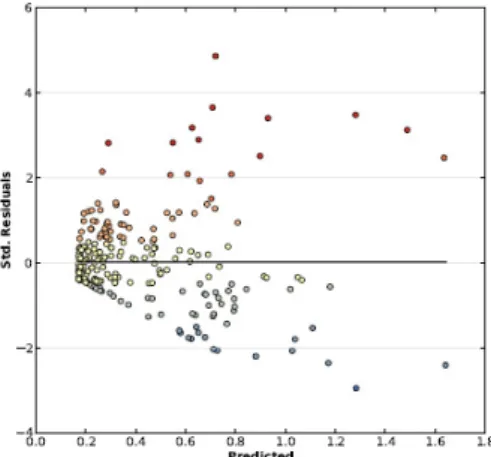
Figure 3 is a scatterplot of standardised error residual values vs. expected screen density values for the OLS model. The cone shape of the dot distribution indicates that the model contains bias due to heteroscedasticity i.e. the relationship between the dependent and the explanatory variables is not consistent in data space. Error residual values are smaller for low screen density values and larger for high screen density values and in general the

(4)

magnitude of under estimation errors (red dots above the line) is greater than the magnitude over estimation errors (blue dots below the line). The colour of the dots matches the legend in Figure 4.

Figure 4 maps the geographic location of the OLS error residuals: over estimations are blue, under estimations are red and yellow indicates small errors. Most error residual cells are shaded yellow and located away from the central CBD zones, indicating the model has predicted screen density relatively accurately in these areas. The strongest coloured red and blue cells are located in central CBD regions, indicating that the model predicts screen density values poorly in these areas. Outlier cells excluded from the screen density dataset are pink and primarily located along the coast line.

Figure 3. Scatterplot of Standard Error Residuals vs. Expected Screen Density Values

Figure 4. Geographical location of Standard Error Residuals

4. Conclusions

All of the spatial analysis tools explored by this study were found to be useful aids when conducting spatial analysis at a global scale, each having its own strengths and weaknesses. Spatial distribution maps allowed the spatial distribution pattern of cinema screen locations and population density to be visualized and facilitated an understanding of the degree to which the two correlated. Spatial autocorrelation statistics provided a statistical measure of the spatial clustering inherent in the screen and population density datasets, particularly Anselin’s local I which indicated both the magnitude and location of clusters and outlier values. Regression analysis was able to numerically assess the correlation between screen and population density, as well as provide an indication of the spatial pattern of the bias present in the model.

A number of limiting factors were identified when conducting this analysis. Boundary misalignments between the cinema and population datasets resulted in the exclusion of some cinemas and the creation of a number of abnormally high outlier values. All cinema screens in the analysis were given an equal weighting, regardless of how many times per day they were viewed and there was a 12 year time misalignment between the SEDAC datasets and the cinema location dataset. Future studies may be able to mitigate these factors using spatial filtering techniques to help smooth boundary misalignments, heteroscedasticity bias may be improved if cinema screens were weighted by their viewing rate and the utilization of a more recent population dataset would address the issue of time misalignment.

In conclusion it was found that a methodology which utilises the above spatial analysis tools in conjunction with a global gridded population dataset, provides a sound framework for investigating the correlation between population distribution and a geographical feature of interest at a global scale. The analysis undertaken was able to visually and

(5)

statistically identify the spatial distribution of cinema screens and population density, as well as establish the degree to which the two features were correlated.

Acknowledgements

This study was conducted as part of Australian Research Council (ARC) project DP120101940.

References

1. Moran, P., The Interpretation of Statistical Maps. Journal of the Royal Statistical Society. 1948. 10(2): p. 9. 2. Anselin, L., Local Indicators of Spatial Association - LISA. Geographical Analysis, 1995. 27(2): p. 23.

3. Center for International Earth Science Information Network - CIESIN - Columbia University, United Nations Food + Agriculture Programme - FAO, and Centro Internacional de Agricultura Tropical - CIAT, Gridded Population of the World, Version 3 (GPWv3): Population Count Grid, 2005, NASA Socioeconomic Data and Applications Center (SEDAC): Palisades, NY.

4.Center for International Earth Science Information Network - CIESIN - Columbia University and Centro Internacional de Agricultura Tropical - CIAT, Gridded Population of the World, Version 3 (GPWv3): Land and Geographic Unit Area Grids, 2005, NASA Socioeconomic Data and Applications Center (SEDAC): Palisades, NY.

5.Center for International Earth Science Information Network - CIESIN - Columbia University and Centro Internacional de Agricultura Tropical - CIAT, Gridded Population of the World, Version 3 (GPWv3): Population Density Grid, 2005, NASA Socioeconomic Data and Applications Center (SEDAC): Palisades, NY.