Nonparametric density estimation: A comparative study
Teruko Takada
Department of Economics, University of Illinois
Abstract
Motivated by finance applications, the objective of this paper is to assess the performance of several important methods for univariate density estimation focusing on the robustness of the methods to heavy tailed target densities. We consider four approaches: a fixed bandwidth kernel estimator, an adaptive bandwidth kernel estimator, the Hermite series (SNP) estimator of Gallant and Nychka, and the logspline estimator of Kooperberg and Stone. We conclude that the logspline and adaptive kernel methods are superior for fitting heavy tailed densities. Evaluation of the convergence rates of the SNP estimator for the family of Student−t densities reveals poor performance, measured by Hellinger error. In contrast, the logspline estimator exhibits good convergence independent of the tail behavior of the target density. These findings are confirmed in a small Monte−Carlo experiment.
A more detailed version of the results described here is available in the first chapter of Takada (2001). I am deeply grateful for many useful comments from Roger Koenker.
Citation: Takada, Teruko, (2001) "Nonparametric density estimation: A comparative study." Economics Bulletin, Vol. 3, No. 16
1. Introduction
The primary objective of this paper is to assess the performance of several univariate density estimators focusing on target densities with heavy tails. Motivated by finance applications, it is particularly important to find methods that perform well for heavy-tailed densities. We consider four approaches: a fixed bandwidth kernel estimator of Sheather and Jones (1991), the adaptive bandwidth kernel estimator of Silverman (1986), the Hermite Series (SNP) method of Gallant and Nychka (1987), and the logspline approach of Kooperberg and Stone (1991, 1992). Primarily, we focus on the simples case of univariate density estimation with i.i.d. observations. In future work we hope to consider extensions to dependent data.
We argue that the logspline and adaptive kernel methods are superior to the other methods for target densities with heavy tails. In particular, the performance of the SNP estimator relative to the logspline estimator becomes significantly worse as the tail of the density becomes heavier. For algebraically tailed densities like the Student-t family the Hellinger error of the logspline estimator with parametric dimension p decreases exponentially in p independent of tail heaviness. On the other hand, the Hellinger error of the SNP estimator decreases algebraically, like p−ν/2, where ν denotes the degrees of freedom of the t-distribution and reflects tail heaviness. These findings are confirmed in a small Monte-Carlo experiment designed to compare the four candidate estimators.
2. The Methods
Given a sample{X1, X2, . . . , Xn}, the classical kernel density estimator with Gaussian kernel has the form
ˆ fF K(x) = 1 nh n i=1 φ x−Xi h , (1)
whereφdenotes the standard Gaussian density, and a fixed bandwidthh controls the degree of smoothing. In selecting h, we use the two-stage direct plug-in bandwidth selection method of Sheather and Jones (1991), which has been shown to perform quite well for many density types by Parkand Turlach (1992) and Wand and Jones (1995).
The adaptive kernel density estimator of Silverman (1986) is defined as ˆ fAK(x) = 1 n n i=1 1 hλiφ x−Xi hλi , (2)
whereλi is a local bandwidth factor which makes the bandwidthλihto narrower near modes and wider in the tails. Based on the pilot estimate by fixed kernel method,
˜
1/2. The bandwidth of the pilot estimate is determined by Silverman’s (1986) rule-of-thumb,h= 0.9An−1/5 whereA= min{standard deviation, interquartile range}/1.34. The Gallant and Nychka (1987) SNP approach is a truncated Hermite series esti-mator which is spanned as
ˆ fSNP(x, θ) = K i=0 θiwi(x) 2 +ε0φ(x), θ = (θ0, . . . , θK), K i=0 θi2+ε0 = 1, (3) where wi(x) is a normalized Hermite polynomial multiplied by the squared root of standard normal density, φ(x) is the standard normal density, and ε0 is a (small) positive number. Estimation is by quasi-maximum likelihood:
ˆ θ = argmaxθ,µ,σ1 n n j=1 log 1 σ ˆf SNP X j −µ σ , θ , (4)
where µ and σ correspond to location and scale. The truncation point is chosen
as either K = n1/5 or according to the AIC or BIC model selection criterion. The parametric dimension is p=K+ 3, due to inclusion of µ,σ, and the θ0 term.
The logspline method of Kooperberg and Stone (1991, 1992) models a log-density function as a cubic spline:
ˆ fLS(x, θ) = exp p i=1 θiBi(x)−c(θ) , x∈ R, (5)
where c(θ) is a normalization factor, and the functions {Bi(x)} denote the standard cubic B-splines. The coefficientsθ are estimated by maximum likelihood; knot selec-tion determining the choice of the B-spline basis is based on the BIC criterion.
3. SNP Convergence Rates for Heavy-Tailed Densities
In this section we consider the change of the SNP (Hermite) approximation error as the number of parameters grows for the family of Student-t densities and derive the rate of convergence of the SNP approximation, as a function of the dimension of SNP model and the degrees of freedom, ν, of the t-density.
3.1 SNP coefficients and Hellinger error
Under certain regularity conditions, a densityf can be represented as an infinite sum of orthonormal Hermite polynomials
f(x, θ) = ∞ i=0 θiwi(x) 2 , θ = (θ0, θ1, . . . .), ∞ i=0 θ2i = 1. (6)
TK(x, λ) = K i=0 λiwi(x), (7)
where λi are arbitrary. The Hellinger error in approximating f(x) by TK(x, λ) is H(f, TK) = ∞ −∞( f(x) − TK(x, λ))2dx. (8)
The coefficients, θi, minimizing Hellinger error can be determined by calculating θi =
∞
−∞
f(x, θ) wi(x)dx. (9)
Using the orthogonality of thewi we have H(f, TK) = 1 + K i=0 (λi −θi)2− K i=0 θi2. (10)
Thus,H(f, TK) is minimized over theλi’s by choosingλi =θi :i= 1, . . . , K. Having chosen the λi in this way we have
H(f, TK) = ∞
i=K+1
θi2, (11)
so ε0 in (3) may be interpreted as the Hellinger error of the SNP estimator with the coefficient determined as in (9).
3.2 Evaluating the approximation error of the SNP estimator.
Let p = K + 3 be the number of parameters of the SNP approximation. We have
computed θp up to p= 200 using (9) for several densities with varying tail behavior: Student-t distributions with degrees of freedom ν = 1, 2, 3, 5, 11, and a bimodal mixture of normal densities.1 In Figure 1, we plot for each of the densities, the logarithm of|θp|as a function ofpon log scale. The plotted curves are asymptotically linear for the Student-t densities, but curved downward for the bimodal density. Moreover, as the degrees of freedom ν decreases, the plotted slope becomes flatter, indicating that the rate of approximation error improvement measured by Hellinger distance becomes slower as the tail of thet-density becomes heavier.
The linearity observation in Figure 1 suggests that for algebraic tailed densities that we have the relation,
θp =Ap−α. (12)
Supposing (12) holds, consider approximating the sum H(f, TK) =∞i=K+1θi2 by the integral h(p) =p∞θ2(v)dv. For (12) we have,
1A mixture of normals such that 1
h(p) = ∞ p θ 2(v)dv=A2 ∞ p v −2αdv=A2(2α−1)p−(2α−1). (13) The value for α corresponds to the slope of the Student-t lines in Figure 1. Based on observations for each of the curves with different degrees of freedom, ν, we esti-mated α for the range of large p by least squares regression. Since the number of observations is limited at largep, estimation is done for several different ranges of p. See Table 1.4 of Takada (2001) for further details. The estimatedα increase exhibit-ing a regular pattern asν increases;α ≈0.75,1.00,1.25,3.25±2ˆσ forν = 1,2,3,5,11, respectively, which relation is summarized as
α ≈(ν+ 2)/4, (14)
over the range of ν studied.
Based on (14), we conclude that Hellinger error decreases like,
h(p)∼p−ν/2, (15)
ifp=nγ is assumed, the Hellinger rate of convergence becomesh∼n−νγ/2. Recently, Coppejans and Gallant (2000) have shown that forp=nγ the best Hellinger error rate for the SNP density estimator ish∼n−kγ/2,wherek is determined by the conditions in the following lemma.
Lemma(Fenton and Gallant, 1996b)Letf be a density such thatf(x) =g2(x)e−x2/2+
0φ(x). If g is k-times differentiable with g(j) ∈ L2(e−x
2/2
) for j = 0,1, . . . , k, then
the Hermite coefficients of g satisfy ∞i=pθ2i =o(p−k).
This result seems to suggest that provided f is sufficiently smooth, as determined by the order of the differentiability,k, the rate of convergence of the SNP approximation is good. While the differentiability of g in the foregoing lemma may be considered quite innocuous, the requirement that thatg(j) ∈L
2(e−x 2/2
), turns out to be surpris-ingly restrictive for the class of heavy tailed f.
Recall that g(j) ∈ L 2(e−x
2/2
) iff −∞∞ (g(j)(x))2 e−x2/2dx < ∞. For the family of Student-tdensities one can verify by straightforward computations that this condition fails for k > ν/2 for even ν and for k >(ν −1)/2 for odd ν. This is easily seen by computing limx→∞g(j)(x) and noting that the integral diverges unless the limit tends to zero. For example, for t(2) we have limg(j)(x) = ∞ for j = 2,3, . . ., so our observation from Figure 2 that Hellinger error declines likep−ν/2, is in perfect accord with the Lemma. For t(3), limx→∞g(2)(x) = √3
π and the limit diverges forj >2, hence
our conclusion from (15) that Hellinger error declines likep−3/2for t(3) is slightly more optimistic than the o(p−1) conclusion of the Lemma. This pattern is sustained for larger ν showing that the failure of the L2 condition is a critical determinant of the performance of the SNP estimator. We note that since our evaluation for whether limx→∞g(j)(x) → ∞ for the Student-t family depends only on the tail behavior of
target densities, the foregoing conclusions may be extended to the general class of densities with algebraic tails.
In this section, we have numerically derived a Hellinger rate of convergence that
depends on the degree of freedom, ν as in equation (15). If we approximate k as
k ∼ν/2 for both even and oddν, ∞i=pθ2
i =o(p−k) in Lemma of Fenton and Gallant
becomes ∞i=pθ2
i = o(p−ν/2) which is consistent with (15) given the relation (11).
Using the connection just established, it is suggested that the convergence of the SNP estimator is highly sensitive to the tail behavior of the target density, with poor performance at heavy tailed densities like the Student-twith low degrees of freedom.
4. Logspline Convergence Rates for Heavy-Tailed Densities
To contrast the SNP results in the previous section with the behavior of the logspline estimator we have computed the Hellinger error of thepdimensional logspline estimator based on artificial observations at equally spaced quantiles of the target density. Modifying the logspline routines of Kooperberg and Stone (1991, 1992), we replace the summation in (5) by integration so that the true density can be ap-proximated, and the effect of knot placement on the rate of convergence is kept to a minimum. The numerically derived Hellinger error of the logspline method in approx-imating the true t(ν) densities is found to decrease faster than p−7, and suggesting an exponential law of the form e−αpβ˜, with parameters independent of tail behavior. For algebraic tailed densities like the Student-t family, this represents a considerable gain over the SNP method.
Figure 2 illustrates our comparison for the case of the t(3) density. The solid line is the Hellinger error for the SNP method in approximating true t(3) density as a function of the number of parameters p as developed in Section 3. The dotted line is the counterpart for the logspline method. The open and filled circles indicate the Monte Carlo simulation results in the next section for the Hellinger error of the logspline method and the SNP method, respectively.
It is seen that the Hellinger approximation error of the logspline method decreases significantly faster than that of the SNP method, and the rate is consistent with the Monte Carlo simulation results.
5. Monte Carlo Simulation Study
This section compares the performance of our four density estimators in fitting heavy-tailed densities in a small Monte Carlo study. In addition to the normal density,t(3) and t(1) densities are chosen to see the effect of tail behavior. The lognormal density is included as different type of heavy tail. All the densities are rescaled so that 99.9% of the mass is included in the range of [−3,3]. We evaluate the performance by the Hellinger error defined as
HM( ˆf , f) = M −M( ˆ f(x)− f(x))2dx. (16)
The Hellinger criterion accentuates the error in the tails. We set M = 3.
The source code used for the Monte-Carlo study for the SNP estimator is that of Fenton and Gallant (1996a), for the logspline method that of Kooperberg and Stone (1991, 1992). The adaptive kernel estimator is based on Silverman (1986). The direct plug-in fixed kernel method is coded by Wand and Jones (1995). In the Monte Carlo, the default settings are used for all the algorithms. The logspline program includes
knot deletion procedure. The numbers of parameters p for the SNP and logspline
estimators are determined to minimize the BIC criterion.2
Table I summarizes the Hellinger performance for each of the densities studied. The sample size is fixed at 500; the error statistics are the average of 500 replications. The errors of the logspline and adaptive kernel methods are quite similar for all the densities. Those of the SNP and fixed kernel methods increase as the tails become heavier. The performance ranking for heavy tailed densities is 1) logspline, 2) adap-tive kernel, 3) fixed kernel, and 4) SNP. In particular, the performance of the SNP estimator relative to that of the logspline estimator becomes significantly worse as the tail of the density becomes heavier.
To assess the qualitative performance in fitting heavy-tailed densities, the t(3) density is estimated using each of the four methods for one realization of a random sample, and the results are illustrated in Figure 3. The dotted lines indicate the true t(3) density while the solid lines denote the estimates. The data range of the particular sample used in Figure 3 is [−3.35,1.23] in the rescaled range where [−3,3] includes 99.9% of the mass. In this particular example, the estimates of right tail diverges for three methods except the SNP since there is no data beyond x > 1.23. It is interesting that the SNP method keeps coming back to the true value with large oscillations where there is no data. Concerning the left tails, the SNP estimate exhibits spurious oscillations, which may be attributed to the effect of the higher order terms in the Hermite expansion. The fixed kernel estimate is also problematic showing a mode in left tail.
6. Empirical Example
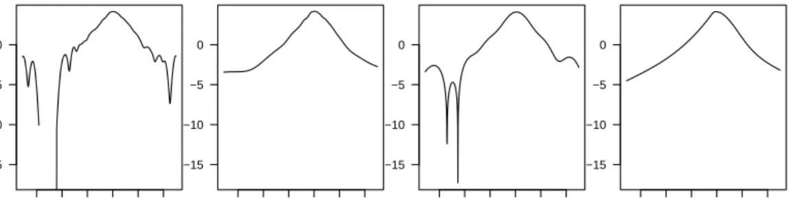
In Figure 4 we compare density estimates for the daily change of S&P500 index. The daily price change is ∆p= logpt−logpt−1. In this figure we observe the same pattern of differences in the tail shape of the estimates exhibited in the previous figure, suggesting that the lobes in the tails of the fixed kernel and SNP estimates are likely to be artifacts of the fitting method rather than real features of the data.
2The upper bound of the Hermite polynomial orderK is set asK =n1/2 to avoid problems of
This observation is relevant to the ongoing dispute over the existence of side lobes in the tails of densities of asset price changes. Based on SNP density estimation of daily pound/dollar exchange rate data from 1974 to 1983, Gallant, Hsieh, and Tauchen (1991) concluded that side lobes existed in the error density of their ARCH specification. Engle and Gonzalez-Rivera (1991) reported similar lobes in the dis-tribution of the standardized residuals from a GARCH(1,1) model. They suggested that the detected side lobes reflect the residual non-linearity which could not be ex-plained by the ARCH/GARCH formulation. In contrast, studies by Bollerslev (1987) and Baillie and Bollerslev (1989) analyzing data on the British pound for 1980-1985, found little evidence against GARCH(1,1) witht-distributed errors. Bollerslev, Chou, and Kroner (1992) suggested that tail oscillations were unduly influenced by a few outliers rather than a feature of the entire sample period. This conclusion seems broadly consistent with the findings reported above.
Note that the price change series are time dependent. Density estimates of weakly dependent data are likely to have larger asymptotic variance than those of i.i.d. data, and thus we need to be more cautious. See, for example, Pagan and Ullah (1999, p43-49).
7. Conclusion
It is clear that for heavy-tailed densities like Student-t, the rate of convergence of the SNP estimator is remarkably slow compared to logspline or even conventional kernel methods. Since financial data are often characterized as heavy-tailed, it seems prudent to consider the logspline methods or adaptive kernel method for financial applications. Extensions and further exploration of these methods for dependent data seem to be promising lines of future research.
References
Baillie, R. T., and T. Bollerslev (1989) ”The Message in Daily Exchange Rates: A Conditional Variance Tale,”Journal of Business and Economic Statistics,7, 297-305. Bollerslev, T. (1987) ”A Conditional Heteroskedastic Time Series Model for Specula-tive Prices and Rates of Return,” Review of Economics and Statistics, 69, 542-547. Bollerslev, T., R.Y.Chou, and K.F.Kroner (1992) ”ARCH Modeling in Finance: A Review of the Theory and Empirical Evidence ”Journal of Econometrics, 52, 5-59. Coppejans, M. and A. R. Gallant (2000) ”Cross Validated SNP Density Estimates,” Manuscript.
Engle, R. F., and G. Gonzalez-Riviera (1991) ”Semiparametric ARCH Models,”
Jour-nal of Business and Economic Statistics, 9, 345-360.
Fenton, V. M. and A. R. Gallant (1996a) ”Qualitative and Asymptotic Performance of SNP Density Estimators,” Journal of Econometrics, 74, 77-118.
Fenton, V. M. and A. R. Gallant (1996b) ”Convergence Rates of SNP Density Esti-mators,” Econometrica,64, 719-127.
Gallant, A. R., D. A. Hsieh, and G. E. Tauchen (1991) ”On Fitting a Recalcitrant
series: The Pound/Dollar Exchange Rate, 1974-1983 ” inNonparametric and
Semi-parametric Methods in Econometrics and Statistics, eds. W. A. Barnett, J. Powell,
and G. E. Tauchen, Cambridge University Press, Cambridge.
Gallant, A. R. and D. W. Nychka (1987) ”Semi-nonparametric Maximum Likelihood Estimation,” Econometrica,55(2), 363-390.
Kooperberg, C. and C. J. Stone (1991) ”A Study of Logspline Density Estimation,”
Computational Statistics & Data Analysis, 12, 327-347.
Kooperberg, C. and C. J. Stone (1992) ”Logspline Density Estimation for Censored Data,” Journal of Computational and Graphical Statistics, 1, 301-328.
Pagan, A. and A. Ullah (1999) Nonparametric Econometrics, Cambridge University
Press.
Park, B. U. and Turlach, B. A. (1992) ”Practical Performance of Several Data Driven Bandwidth Selectors (with Discussion)” Computational Statistics, 7, 251-85.
Sheather, S. J. and M. C. Jones (1991). ”A Reliable Data-Based Bandwidth Selection Method for Kernel Density Estimation,” Journal of the Royal Statistical Society, Series B, 53, 683-690.
Silverman, B.W. (1986) Density Estimation for Statistics and Data Analysis, Chap-man and Hall, London.
Takada, T. (2001) Density Estimation for Robust Financial Econometrics, PhD the-sis, University of Illinois at Urbana-Champaign.
Figure 1: The coefficients of Hermite polynomial terms of the SNP estimates as a function of the number of parameters in approximating true densities.
1 2 5 10 20 50 100 200 500 −15
−10 −5 0
The number of parameters, p (log scale)
log | θ | t(1) t(2) t(3) t(5) t(11) Bimodal
Figure 2: The Hellinger error as a function of the number of parameters.
1 2 5 10 20 50 100 200 −14 −12 −10 −8 −6 −4 −2 0
The number of parameters, p (log scale)
Log Hellinger error
<−− SNP (approx.) Logspline (approx.) −−> Logspline (MC) | | | SNP (MC) n=100 n=500 n=1000
Points labeled as “MC” indicate the Hellinger error results from the Monte Carlo study in Table I. Open circles represent the Monte-Carlo performance of the logspline estimator, filled circles the performance of the SNP estimator. Lines labeled as “approx.” plot the change in the Hellinger error aspgrows in approximating true t(3) density.
Table I: Simulation Results for Densities with Heavy Tails
(Sample size 500, average of 500 simulated samples.)
Normal t(3) t(1) Lognormal
Method mean (s.d.) mean (s.d.) mean (s.d.) mean (s.d.)
F.Kernel 0.0035 (0.0017) 0.0112 (0.0026) 0.1344 (0.0061) 0.0237 (0.0032) Hellinger A.Kernel 0.0035 (0.0016) 0.0049 (0.0020) 0.0247 (0.0038) 0.0121 (0.0022) SNP 0.0010 (0.0010) 0.0111 (0.0069) 0.4242 (0.2946) 0.0383 (0.0168) Logspline 0.0029 (0.0016) 0.0045 (0.0026) 0.0087 (0.0038) 0.0052 (0.0025) p SNP 3.0 (0.0) 10.9 (4.2) 25.3 (1.5) 22.9 (2.9) Logspline 4.2 (0.6) 6.2 (0.5) 9.4 (0.8) 5.8 (1.0)
Figure 3: Estimates of t(3) log densities.
−3 −2 −1 0 1 2 3 −8 −6 −4 −2 0 2 Fixed Kernel
Log density, log f(x)
x −3 −2 −1 0 1 2 3 −8 −6 −4 −2 0 2 Adaptive Kernel x −3 −2 −1 0 1 2 3 −8 −6 −4 −2 0 2 SNP x −3 −2 −1 0 1 2 3 −8 −6 −4 −2 0 2 Logspline x
Dotted lines indicate the truet(3) density; solid lines denote the estimates. Note that they are rescaled so that 99.9% of the mass is included in the range of [−3,3]. The data range for this particular sample is [−3.35,1.23].
Figure 4: Four density estimates for daily changes in S&P500 index.
−0.06 −0.02 0.02
−15 −10 −5 0
Log density, log f(
∆ p) ∆p Fixed Kernel −0.06 −0.02 0.02 −15 −10 −5 0 ∆p Adaptive Kernel −0.06 −0.02 0.02 −15 −10 −5 0 ∆p SNP −0.06 −0.02 0.02 −15 −10 −5 0 ∆p Logspline