S 0025-5718(XX)0000-0
.
CHEBYSHEV ROOTFINDING VIA COMPUTING EIGENVALUES OF COLLEAGUE MATRICES: WHEN IS IT STABLE?
VANNI NOFERINI AND JAVIER P´EREZ
Abstract. Computing the roots of a scalar polynomial, or the eigenvalues of a matrix polynomial, expressed in the Chebyshev basis{Tk(x)} is a fun-damental problem that arises in many applications. In this work, we analyze the backward stability of the polynomial rootfinding problem solved with col-league matrices. In other words, given a scalar polynomialp(x) or a matrix polynomialP(x) expressed in the Chebyshev basis, the question is to deter-mine whether the whole set of computed eigenvalues of the colleague matrix, obtained with a backward stable algorithm, like the QR algorithm, are the set of roots of a nearby polynomial or not. In order to do so, we derive a first order backward error analysis of the polynomial rootfinding algorithm using colleague matrices adapting the geometric arguments in [A. Edelman and H. Murakami,Polynomial roots for companion matrix eigenvalues, Math. Comp. 210, 763–776, 1995] to the Chebyshev basis. We show that, if the absolute value of the coefficients ofp(x) (respectively, the norm of the coeffi-cients ofP(x)) are bounded by a moderate number, computing the roots of
p(x) (respectively, the eigenvalues ofP(x)) via the eigenvalues of its colleague matrix using a backward stable eigenvalue algorithm is backward stable. This backward error analysis also expands on the very recent work [Y. Nakatsukasa and V. Noferini,On the stability of computing polynomial roots via confeder-ate linearizations, To appear in Math. Comp.] that already showed that this algorithm is not backward normwise stable if the coefficients of the polynomial
p(x) do not have moderate norms.
1. Introduction
A popular way to compute the roots of a monic polynomial expressed in the monomial basis is via the eigenvalues of its companion matrix. This is, for in-stance, the way followed by the MATLAB commandroots, that, after balancing the companion matrix, uses the QR algorithm to get its eigenvalues. The numerical properties of this method for computing roots of polynomials have been extensively studied [8, 9, 15, 25], in particular with respect to conditioning and backward errors. It has been shown that, in practice, if the companion matrix is balanced [21], the rootfinding method using companion matrices is numerically stable, in the sense that the computed roots are the exact roots of a nearby polynomial. However,
Received by the editor December 9, 2015.
2010Mathematics Subject Classification. 65H04, 65H17, 65F15, 65G50.
Key words and phrases. polynomial, roots, Chebyshev basis, matrix polynomial, colleague matrix, backward stability, polynomial eigenvalue problem, Arnold transversality theorem.
The work of Vanni Noferini was supported by European Research Council Advanced Grant MATFUN (267526).
The work of Javier P´erez was supported by Engineering and Physical Sciences Research Council grant EP/I005293.
c
XXXX American Mathematical Society
as it was made famous by Wilkinson [22, 26, 27], polynomial roots that lie on a real interval can be highly sensitive to perturbations in the coefficients when the monomial basis is used. So, even perturbations in the coefficients of order of the machine precision may produce a catastrophically large forward error. In practice, rootfinding on a real interval is a very frequent and important situation, and one way to circumvent this problem is to use, instead, a polynomial basis such that the roots of a polynomial expressed in that basis are better conditioned functions of its coefficients, like theChebyshev basis.
Chebyshev polynomials are a family of polynomials, orthogonal with respect to the weight function w(x) = (1−x2)−1/2 on the interval [−1,1], which may be
computed using the following recurrence relation [1, Chapter 22]:
T0(x) = 1, T1(x) =x, and,
Tk(x) = 2xTk−1(x)−Tk−2(x), fork≥2.
(1.1)
Moreover, the Chebyshev polynomialsT0(x), T1(x), . . . , Tn(x) form a basis for the vector space of polynomials of degree at mostnwith real coefficientsRn[x]. Hence, any real polynomialp(x)∈Rn[x] can be written uniquely asp(x) =Pnk=0akTk(x). Chebyshev polynomials are widely used in many areas of numerical analysis, and in particular approximation theory [23]. In fact, a common approach, as done in Chebfun [24], for computing the roots of a nonlinear smooth function f(x) on an interval is to approximate first f(x) by a polynomial p(x) expressed in the Chebyshev basis via Chebyshev interpolation and then compute the roots ofp(x) as the eigenvalues of its colleague matrix [11]. Also, computing the eigenvalues of matrix polynomials in the Chebyshev basis is becoming an important problem [10]. In this paper, we are interested in the backward stability of the rootfinding problem (or of the matrix polynomial eigenvalue problem) solved via colleague matrices and a backward stable eigenvalue algorithm. Our work is motivated by [18], which addresses related issues for confederate matrices (the colleague matrix is a particular example of a confederate matrix [4, 17]). Also, similar backward error analysis may be found in [8, 13, 14]. In [8], the authors study the backward stability of rootfinding methods using Fiedler companion matrices of monic polynomials expressed in the monomial basis; in [13], the authors study the backward stability of rootfinding methods using a suitable companion matrix of polynomials expressed in barycentric form; in [14], several bases are analyzed at once, for nonstandard linearizations of larger size with respect to the colleague or the companion.
Given ap×pmonic matrix polynomial in the Chebyshev basis of degreen
(1.2) P(x) =IpTn(x) + n−1
X k=0
AkTk(x), withAk ∈Rp×p, fork= 0,1, . . . , n−1, where by monic in the Chebyshev basis we mean that the coefficient of Tn(x) is equal toIp (thep×pidentity matrix), thepolynomial eigenvalue problem consists of finding the eigenvalues ofP(x), that is, finding the roots of the scalar polynomial det (P(x)) (note that the monicity ofP(x) implies its regularity, that is, det (P(x)) is not identically zero). For the sake of simplicity of exposition, we focus on poly-nomials with real coefficients, as they are most common in practice when dealing
with the Chebyshev basis; however, the analysis of this paper can be extended to the complex case.
A common approach to solve the polynomial eigenvalue problem forP(x) is to use the block colleague matrix
(1.3) CT = 1 2 −An−1 −An−2+Ip −An−3 · · · −A2 −A1 −A0 Ip 0 Ip 0 · · · 0 0 Ip 0 Ip . .. ... .. . . .. . .. . .. ... . .. ... .. . . .. . .. ... . .. 0 0 · · · 0 Ip 0 Ip 0 · · · 0 2Ip 0 ∈Rnp×np,
since it is known (see [2]) that the eigenvalues of (1.3) coincide with the eigenvalues ofP(x).
The eigenvalues of P(x) may be computed as the eigenvalues of CT using, for instance, the QR algorithm. The QR algorithm is a backward stable algorithm, this means than the computed eigenvalues are the exact eigenvalues of a matrix
CT+E, where Eis a (possibly dense) matrix such that kEk=O(u)kCTk,
for some matrix norm, whereudenotes the machine precision. However, the previ-ous equation does not guarantee that the computed eigenvalues are the eigenvalues of a nearby matrix polynomial of P(x) or, in other words, that this polynomial eigensolver is backward stable. In order for the method to be backward stable (in a normwise sense), the computed eigenvalues should be the exact eigenvalues of a polynomialPe(x) =IpTn(x) +Pkn=0−1AekTk(x),such that
kPe−Pk
kPk =O(u), for some matrix polynomial norm.
In the scalar polynomial case (p= 1), the backward stability of the polynomial rootfinding in degree-graded basis using confederate matrices is studied in [18]. In particular (see [18, Theorem 4.2]), the authors prove that if CT is the colleague matrix of a polynomialp(x) and E∈Rn×n is any matrix, then the eigenvalues of
CT+E are the exact roots of a polynomialpe(x) such that (1.4) pe(x)−p(x) =
n−1
X i=0
δi(p, E)Ti(x) +O(kEk22),
where, for i = 0,1, . . . , n−1, the quantity δi(p, E) is an affine function of the coefficients ofp(x), and, separately, of the entries ofE.
Equation (1.4) implies that if the roots ofp(x) are computed as the eigenvalues of its colleague matrixCT using a backward stable eigenvalue algorithm, then, the computed roots will be the exact roots of a polynomialpe(x) such that
kpe−pk
for some constant k(n). The previous equation shows, first, that this method is not backward stable ifkpk ≫1, and, second, that this method is backward stable if the following two conditions are satisfied: (i) the quantityκ(n) is a low-degree polynomial innwith moderate coefficients; and, (ii) the normkpkis moderate. As it is observed in [18], writingδi(p, E) =Pi,j,ℓβijℓaℓEij, since it is not clear what exactly are the constantsβijℓinvolved, in principle it could happen that|βijℓ| ≫1, implying that κ(n) might not be a polynomial in n with moderate coefficients. However, in this work we show that, in fact,|βijℓ| ≤4, and, so,
kpe−pk
kpk =O(u)kpk,
holds. The previous equation implies that computing the roots of p(x) via the eigenvalues of its colleague matrix using a backward stable eigenvalue algorithm is a backward stable rootfinding algorithm, provided thatkpk.1.
Moreover, using some arguments inspired by [3, 9, 15, 16] we will generalized the previous result to the matrix polynomial case, that is, if the eigenvalues of a matrix polynomial P(x) are computed as the eigenvalues of its colleague matrix using a backward stable eigenvalue algorithm, then, we prove that the computed eigenvalues are the exact eigenvalues of a monic matrix polynomial in the Chebyshev basisPe(x) such that
kPe−Pk
kPk =O(u)kPk.
The previous equation implies that this method is backward stable if kPkis mod-erate.
The paper is organized as follows. At the beginning of Section 2 we present Arnold transversality theorem for colleague matrices, which will be the main tool to study the polynomial backward stability of the rootfinding method using colleague matrices. Then, in Section 2.2 we prove Arnold transversality theorem for colleague matrices, and in Section 2.3 we use this theorem to study the backward stability of the rootfinding method using colleague matrices.
Throughout this paper, for ap×pmatrix polynomialP(x) =Pnk=0AkTk(x), non necessarily monic,kPkF is the norm on the vector space ofp×pmatrix polynomials of degree less than or equal tondefined as
kPkF = v u u t n X k=0 kAkk2F.
Notice that, since we are going to deal with monic polynomials in the Chebyshev basis,An =Ip. Also notice that for a scalar polynomialp(x) =Pnk=0akTk(x), that is, forp= 1, this norm reduces to the usual 2-norm:
kpkF =kpk2= v u u t n X k=0 |ak|2.
2. Arnold transversality theorem for colleague matrices and backward error analysis
Arnold transversality theorem will be the main tool in this section to study what kind of polynomial backward stability is provided by matrix backward stabil-ity when the roots of scalar polynomials or the eigenvalues of matrix polynomials are computed as the eigenvalues of its colleague matrix with a backward stable eigenvalue algorithm. This theorem was first stated in [3] for companion matrices, and later generalized in [18] to confederate matrices of scalar polynomials.
Following [3, 8, 9, 15, 18], we consider the Euclidian matrix spaceRn×n with the usual Frobenius inner product
< A, B >:= tr (ABT),
where MT denotes the transpose of M ∈Rn×n. In this space, the set of matrices similar to a given matrix A ∈ Rn×n is a differentiable manifold in Rn×n. This manifold is called the orbit ofAunder the action of similarity:
O(A) :={SAS−1 : S∈Rn×n and det(S)6= 0}.
A first-order expansion shows that the tangent space ofO(A) atA is the set
TAO(A) :={AX−XA for some X∈Rn×n}.
We also consider the vector subspace of “first block row matrices”, denoted by BFRn,p ⊂ Rnp×np, which is defined as those n×n block matrices [Xij], with
Xij∈Rp×p, whose block rows are all zero except (possibly) the first: BFRn,p:= n X =IP 0 · · · 0 T X1 X2 · · · Xn for some X1, X2, . . . , Xn∈Rp×p o ⊂Rnp×np.
Note that takingp= 1 the spaceBFRn,p reduces to the vector subspaceFRn of “first row matrices” introduced in [18].
Arnold transversality theorem for a block colleague matrixCT of a monic matrix polynomial P(x) in the Chebyshev basis states that any matrixE ∈Rnp×np may be decomposed as
E=F0+T,
where F0 ∈ BFRn,p is a first block row matrix and T ∈TCTO(CT). Notice that
takingp= 1 in the previous decomposition, this “block” version of Arnold transver-sality theorem reduces to a special case of [18, Theorem 4.1].
In Section 2.3 we present a proof of Arnold transversality theorem, different to the one in [18], extending (for the important case of the Chebyshev basis) [18, The-orem 4.1] to the more complicated case of matrix polynomials. The new approach allows us to compute explicitly the matrix F0. Then, using this explicit
expres-sion, we study the polynomial backward stability of the rootfinding method using colleague matrices.
2.1. Clenshaw shifts and Clenshaw matrices. In this section we introduce some matrix polynomials and some matrices, named here as Clenshaw shifts and Clenshaw matrices, respectively, associated with a monic matrix polynomial in the Chebyshev basisP(x), that will be used through Section 2.3 and will be key in the following developments. Clenshaw shifts are the generalization of the Horner shifts (see [7]) when the polynomialP(x) is expressed in the Chebyshev basis.
Associated with thep×pmonic matrix polynomial in the Chebyshev basisP(x) in (1.2), we define the followingp×pmatrix polynomials:
H0(x) = 2Ip,
H1(x) = 2xH0(x) + 2An−1,
Hk(x) = 2xHk−1(x)−Hk−2(x) + 2An−k, fork= 2,3, . . . , n−2,
Hn−1(x) =xHn−2(x)−Hn−3(x)/2 +A1.
(2.1)
We will refer, fork = 1,2, . . . , n, to the matrix polynomialHk(x) as the degree k Clenshaw shift of P(x), since for p= 1 they coincide with the well known Clen-shaw shifts associated with a scalar polynomial expressed in the Chebyshev basis [6]. Clenshaw shifts are related with the polynomial P(x) through the following equation [6]:
(2.2) 2P(x) = 2xHn−1(x)−Hn−2(x) + 2A0.
In Theorem 2.1, given the Chebyshev polynomialTn−i(x) and the Clenshaw shift
Hn−k(x), we show how to expressTn−i(x)Hn−k(x) uniquely asQij(x)+rik(x)P(x), whereQij(x) is ap×pmatrix polynomial of degree less than or equal ton−1 and
rik(x) is a scalar polynomial. The proof of Theorem 2.1 is elementary but rather technical, so we leave it to the appendix. In order to write down a reasonably simple formula forTn−i(x)Hn−k(x), we define the following quantities
Γ2k+1= Γ2k−1+ 2An−2k−1, fork= 1,2, . . . , jn 2 k −1, with Γ0= 2Ip, and Γ2k = Γ2(k−1)+ 2An−2k, fork= 1,2, . . . , ln 2 m −1, with Γ1= 2An−1. (2.3)
Notice that in Γk only appear coefficients ofP(x) with indices of the same parity. Theorem 2.1. LetP(x) =IpTn(x) +Pnk=0−1AkTk(x)be ap×pmonic matrix poly-nomial in the Chebyshev basis of degreen, letTn−i(x)andHn−k(x)be, respectively, the degreen−iChebyshev polynomial and the degreen−kClenshaw shift ofP(x), withi, k∈ {1,2, . . . , n}. Then, there exist a uniquep×pmatrix polynomialQik(x) of degree less than or equal ton−1and a unique scalar polynomialrik(x)such that
Tn−i(x)Hn−k(x) =Qik(x) +rik(x)P(x), where, • ifi≥n−k+ 1 andk≥2, (2.4) Qik(x) = n−Xk−1 ℓ=0 Γℓ(T2n−i−k−ℓ(x) +T|k+ℓ−i|(x)) + Γn−kTn−i(x); • ifi=nandk= 1, (2.5) Qik(x) = nX−2 ℓ=0 ΓℓTn−1−ℓ(x) + Γn−1 2 T0(x);
• if i≤n−kandn−1≥k≥2, Qik(x) = i−2 X ℓ=0 Γℓ(Ti+k−2−ℓ(x) +T|k+ℓ−i|(x)) + Γi−1Tk−1(x) − n−Xk+1−i ℓ=1 k−X1+ℓ r=1 2Ak−1+ℓ−rT|n−i+1−ℓ−r|(x); (2.6) • ifi≤n−kandk= 1 Qik(x) = i−2 X ℓ=0 ΓℓTi−1−ℓ(x) + Γi−1 2 T0(x)− n−i X ℓ=1 ℓ X r=1 Aℓ−rT|n−i+1−ℓ−r|(x); (2.7)
whereΓℓ, for ℓ= 0,1,2, . . ., is defined in (2.3).
From Theorem 2.1, it is clear that there exists a unique n×n block matrix
Mk= [(Mk)ij], with (Mk)ij∈Rp×p, such that, fork= 1,2, . . . , n,
(2.8) Tn−1(x) .. . T1(x) T0(x) ⊗Hn−k(x) =Mk Tn−1(x) .. . T1(x) T0(x) ⊗Ip+ r1k(x) .. . rn−1,k(x) rnk(x) ⊗P(x),
where⊗denotes the Kronecker product, for some scalar polynomialsr1k(x), . . . , rnk(x). We will refer to the matrixMk in (2.8) as thekth Clenshaw matrix ofP(x).
By direct multiplication, it may be easily checked that the block colleague matrix
CT satisfies (2.9) x Tn−1(x) .. . T1(x) T0(x) ⊗Ip=CT Tn−1(x) .. . T1(x) T0(x) ⊗Ip+ 1 2e1⊗P(x).
Equations (2.8) and (2.9) shows that the Clenshaw matrices and the colleague matrix can be interpreted, respectively, as the multiplication-by-Clenshaw shifts and the multiplication-by-x operators in certain quotient modules (see also [19, Sec. 5]).
Using (2.8) and (2.9), in Proposition 2.2 we show that the Clenshaw matrices
M1, M2, . . . , Mn in (2.8) satisfy a simple recurrence relation.
Proposition 2.2. Let P(x) =IpTn(x) +Pnk=0−1AkTk(x)be a p×pmonic matrix polynomial in the Chebyshev basis of degree n, letCT be the block colleague matrix of P(x), and letM1, M2, . . . , Mn be the Clenshaw matrices in (2.8). Then,
Mn=In⊗2Ip,
Mn−1= 2MnCT +In⊗2An−1,
Mk= 2Mk+1CT −Mk+2+In⊗2Ak, for k=n−2, . . . ,3,2, and
M1=M2CT −M3/2 +In⊗A1.
Proof. The proof proceeds backwards fromk=n. First, we prove that the result is true fork=n. From (2.1), we have
Tn−1(x) .. . T1(x) T0(x) ⊗H0(x) = Tn−1(x) .. . T1(x) T0(x) ⊗2Ip= 2Ip . .. 2Ip 2Ip Tn−1(x) .. . T1(x) T0(x) ⊗Ip.
Comparing the previous equation with (2.8), we deduce thatMn=In⊗2Ip. Second, we prove that the result is true fork=n−1. From (2.1), we have Tn−1(x) .. . T1(x) T0(x) ⊗H1(x) = Tn−1(x) .. . T1(x) T0(x) ⊗(2xH0(x) + 2An−1) = 2x Tn−1(x) .. . T1(x) T0(x) ⊗H0(x)+ Tn−1(x) .. . T1(x) T0(x) ⊗2An−1.
Using (2.8) withk=n, together with (2.9), we get Tn−1(x) .. . T1(x) T0(x) ⊗H1(x) = (2MnCT+In⊗2An−1) Tn−1(x) .. . T1(x) T0(x) + r1,n−1(x) .. . rn−1,n−1(x) rn,n−1(x) ⊗P(x),
for some scalar polynomialsr1,n−1(x), . . . , rn,n−1(x). Comparing the previous
equa-tion with (2.8), we deduce thatMn−1= 2MnCT +In⊗2An−1.
Third, we prove that the result is true forn−2≥k≥2. From (2.1), we have Tn−1(x) .. . T1(x) T0(x) ⊗Hn−k(x) = Tn−1(x) .. . T1(x) T0(x) ⊗(2xHn−k−1(x)−Hn−k−2(x) + 2Ak) = 2x Tn−1(x) .. . T1(x) T0(x) ⊗Hn−k−1(x)− Tn−1(x) .. . T1(x) T0(x) ⊗Hn−k−2(x) + Tn−1(x) .. . T1(x) T0(x) ⊗2Ak.
Using (2.8) withk+ 1 andk+ 2, together with (2.9), we get Tn−1(x) .. . T1(x) T0(x) ⊗Hn−k(x) =(2CTMk+1−Mk+2+In⊗2Ak) Tn−1(x) .. . T1(x) T0(x) + r1k(x) .. . rn−1,k(x) rn,k(x) ⊗P(x),
for some scalar polynomials r1k(x), . . . , rnk(x). Comparing the previous equation with (2.8), we deduce thatMk= 2CTMk+1−Mk+2+In⊗2Ak.
Finally, the proof of the last case (k= 1) is similar to the proof for the previous cases (n−2 ≥k ≥2), but using Hn−1(x) =xHn−2(x)−Hn−3(x)/2 +A1, so we
omit it.
Remark 2.3. Clenshaw matrices are closely related with the so called Leverrier’s algorithm for orthogonal polynomial bases[5], which allows the simultaneous deter-mination of the characteristic polynomial of a matrix A and the adjoint matrix of
xI−A. Indeed, if we consider a scalar polynomial p(x) =Tn(x) +Pnk=0−1akTk(x), it may be checked that the adjoint of zI−CT is given by
(2.11) adj (xI−CT) = 1 2n−1 nX−1 k=0 Mk+1Tk(x), whereM1, M2, . . . , Mn are the Clenshaw matrices of p(x).
The Clenshaw matricesM1, M2, . . . , Mnhave a complicated structure. We illus-trate this with an example of moderate size. For n = 6 and k = 3, it is easy to check using (2.10) that the matrixMk is equal to
0 −2A2 −2A3−2A1 2Ip−2A4−2A2−4A0 −2A3−4A1 −2A2−2A0 0 0 2Ip−2A2 2A5−2A3−2A1 2Ip−2A2−4A0 −2A1 0 2Ip 2A5 2Ip+ 2A4−2A2 2A5−2A1 2Ip−2A0 2Ip 2A5 2Ip+ 2A4 2A5+ 2A3 4Ip+ 2A4 2A5 0 2Ip 2A5 4Ip+ 2A4 4A5+ 2A3 2A4+ 2Ip 0 0 4Ip 4A5 4Ip+ 4A4 2A5+ 2A3 .
Two observations about the block matrix above are: (i) its first block column is equal to en−k+1⊗2Ip, where eℓ denotes the ℓth column of the n×n identity matrix; and, (ii) if we setAn :=Ip, each block entry has the formPni=0ciAi, where |ci| ≤4. In Theorem 2.4, we show that the two previous observations are true for anynandk. Property (i) will be key to prove Arnold transversality theorem, and property (ii) will be key to study what kind of backward stability of a linearization-based algorithm for the polynomial eigenvalue problem is provided by the backward stability of an eigensolver for the linearized problem.
Theorem 2.4. Let P(x) = IpTn(x) +Pnk=0−1AkTk(x) be a p×p monic matrix polynomial in the Chebyshev basis of degree n, and letMk, for k = 1,2, . . . , n, be the kth Clenshaw matrix in (2.8). Then, the following statements hold:
(a) The first block column ofMk is equal toen−k+1⊗2Ip, whereeℓdenotes the
ℓth column of then×n identity matrix.
(b) ForP i, j = 1,2, . . . , n, the (i, j)th block entry of Mk satisfies (Mk)ij = n
t=0αt,ijkAtwith |αt,ijk| ≤4, where we set An:=Ip.
Proof. From Theorem 2.1 together with (2.8), we have Hn−k(x)Tn−i(x) = Pnj=1(Mk)ijTn−j(x) +rik(x)P(x). Therefore, to prove part (a) it is enough to show that
(2.12) Tn−i(x)Hn−k(x) = 2IpTn−1(x) +· · ·+rik(x)P(x), ifi=n−k+ 1, and that
(2.13) Tn−i(x)Hn−k(x) = (Mk)iνTν(x) +· · ·+rik(x)P(x),
withν < n−1, ifi6=n−k+1, where the dots correspond to Chebyshev polynomials with lower indices.
First, suppose that i≥n−k+ 1. We will prove thatTn−i(x)Hn−k(x) is of the form (2.12) wheni=n−k+ 1 and it is of the form (2.13) otherwise. We need to distinguish several cases. First, letk=n. From (2.4) we get thatTn−i(x)H0(x) =
Γ0Tn−i(x) = 2IpTn−i(x). Since the indexn−iis equal ton−1 if and only ifi= 1, the result is true in this case. Then, consider the casen−1≥k≥2. There are three kinds of indices of Chebyshev polynomials in (2.4). The first is 2n−i−k−ℓ, which is equal to n−1 if and only if ℓ= 0 and i=n−k+ 1. This gives a contribution Γ0Tn−1(x) = 2IpTn−1(x) only wheni=n−k+ 1. The second one is |k+ℓ−i|.
Taking into account the possible values thatk,ℓ, andican take in (2.4), it may be easily checked that this index is smaller than or equal ton−2. The third index is
n−iwhich necessarily is smaller than or equal to n−2, and, hence, the result is true in this case. Finally, consider the casek= 1 andi=n. There are two kinds on indices of Chebyshev polynomials in (2.5). The first one isn−1−ℓ, which is equal to n−1 if and only ifℓ = 0. This gives a contribution Γ0Tn−1(x) = 2IpTn−1(x).
The second index is 0, which is smaller than n−2. Therefore, the result is also true in this case.
Now suppose that i≤n−k. We will we prove that Tn−i(x)Hn−k(x) is of the form (2.13). Notice that there are four kinds of indices in (2.6) whenk≥2, namely,
i+k−2−ℓ,|k+ℓ−i|,|n−i+ 1−ℓ−r|andk−1, and three kinds on indices in (2.7) whenk= 1, namely,i−1−ℓ,i−1 and|n−i+ 1−ℓ−r|. Taking into account the possible values that k, ℓ,r, andi can take in (2.13), in both cases (k≥2 and
k= 2), it may be checked that these indices do not exceed n−2.
Now, we proceed to prove part (b). Again, we need to distinguish several cases. First, suppose thati≥n−k+ 1 and also assume thatk≥2 (the argument when
k= 1 is similar and simpler, so we omit it), and consider the three kinds of indices of Chebyshev polynomials that appear in (2.4), namely, 2n−i−k−ℓ,|k+ℓ−i|, and n−i. For ℓ = 0,1, . . . , n−k, a careful look at these indices reveals that if
k+ℓ−i≥0, then the three of them are different. Therefore, we can write (2.4) as (2.14) n−1 X ℓ=0 BℓTℓ(x) + −1 X ℓ=−(1−n) BℓT−ℓ(x),
where Bℓ is equal to either 0 or Γt for some t. It follows that (Mk)ij is equal to either 0, Γt for somet, or Γt1+ Γt2 for somet1, t2. Finally, recall from (2.3) that
Γtis equal to 2Ip+ 2An−2+ 2An−4+· · · iftis even, or to 2An−1+ 2An−3+· · · if tis odd. Therefore, (Mk)ij =Pnt=0αt,ijkAt, with |αt,ijk| ≤4.
Then suppose thati≤n−k and also assume thatk≥2 (again, the argument when k= 1 is similar and simpler, so we omit it). First, consider the three kinds of indices of Chebyshev polynomials that appear in the first summand in (2.6), namely, i+k−2−ℓ, |k+ℓ−i|,k−1. Forℓ = 0,1, . . . , i−2, again, it may be checked that if k+ℓ−i ≥ 0, then these three indices are different. Therefore, the first summand in (2.6) is also of the form (2.14). Finally, consider the index of the Chebyshev polynomials and the index of the coefficients Ai that appear in the second summand in (2.6), namely, |n−i+ 1−ℓ−r|, and k+ 1 +ℓ−r. If
n−i+ 1−ℓ−r ≥0, it may be checked that for any two allowed different pairs (ℓ, r) that realize the same value of n−i+ 1−ℓ−r, then the associate indices
k+ 1 +ℓ−rmust be different. Since the same occur whenn−i+ 1−ℓ−r <0, it follows that (2.6) is of the form
nX−2 ℓ=0 CℓTℓ(x) + −1 X ℓ=−(2−n) CℓT−ℓ(x)−2 n−2 X ℓ=0 DℓTℓ(x)−2 −1 X ℓ=2−n DℓT−ℓ(x) +rik(x)P(x) whereCℓ is equal to either 0 or Γt for somet, and Dℓ is equal toPq
ℓ
t=1Ait, where
it16=it2 whenevert16=t2. Then, it follows that (Mk)ij = n X ℓ=0 δℓAℓ− n X ℓ=0 ρℓAℓ,
where δℓ and ρℓ are equal to either 4, or 2 or 0, therefore (Mk)ij =Pnt=0αt,ijkAt
with|αt,ijk| ≤4.
If necessary, explicit expressions of the entries of the Clenshaw matricesM1, M2, . . . , Mn may be obtained from Theorem 2.1. However, since Theorem 2.4 is the only information that we will need about them to prove our main results in the following section, we do not pursue that idea.
2.2. Proof of Arnold transversality theorem for colleague matrices. In this section we prove Arnold transversality theorem for colleague matrices of monic polynomials in the Chebyshev basis. That is, we show that any matrixE∈Rpn×pn
may be decomposed as
(2.15) E=F0+T,
where F0 ∈ BFRn,p is a first block row matrix and T ∈TCTO(CT), constructing
the matrixF0 explicitly.
As in the case of the monomial basis, generically, dim (TCTO(CT))+dim (BFRn,p)
=n2p2−np+np2 ≥n2p2 (see [9, 16]). In words, the tangent space T
CTO(CT)
and the vector space of first block row matrices BFRn,p may have a nontrivial intersection when p > 1. For this reason, following [9, 16] we choose a particular subspace of the tangent space that will give a unique decomposition (2.15). This subspace is denoted by Sub TCTO(CT) and it is given by
SubTCTO(CT) ={X∈TCTO(CT) such that X has 0 first block column}.
In order to get the decomposition (2.15) withT ∈SubTCTO(CT) we will make
use of the Clenshaw matrices M1, M2, . . . , Mn ∈ Rnp×np, defined in (2.8), of the matrix polynomialP(x) in (1.2). Though the only information that we need about
Clenshaw matrices are those stated in Theorem 2.4 together with the recurrence relation (2.10).
Following [9], we also define theblock traceof anp×npblock matrixZ= [Zij], withZij ∈Rp×p, as thep×pmatrix
trp(Z) := n X i=1
Zii.
The block trace is used in Theorem 2.5, which provides a characterization of the subspace SubTCTO(CT), and is a generalization of [9, Theorem 4.1] when the
matrix polynomialP(x) is expressed in the Chebyshev basis.
Theorem 2.5. For any Z∈Rpn×pn,
(2.16) trp(Mk+1Z) = 0, for k= 0,1, . . . , n−1,
if and only if
(2.17) Z=CTX−XCT for someX ∈Rnp×np with 0 first block column. Moreover, either condition determines the first block row of Z uniquely given the remaining block rows.
Proof. From part (a) in Theorem 2.4, the (n−k,1) block entry of Mk+1 is equal
to 2Ip, and the (i,1) block entry ofMk+1, withi6=n−k, is equal to 0. Therefore, Z1,n−k, fork= 0,1, . . . , n−1, is uniquely determined from (2.16). Also, ifX has 0 first block column, it may be easily checked that the map fromX to the lastn−1 block rows ofCTX−XCT has a trivial nullspace. Thus,Z is uniquely determined by (2.17).
To finish the proof we need to prove that (2.17) implies (2.16). That is, we need to show that trp(Mk+1(CTX−XCT)) = 0 for any block matrix X with 0 first block column. In order to do this, first, we show that ifX has 0 first block column, then trp(Mk+1XCT) = trp(CTMk+1X). The proof of the previous equation is not
completely immediate whenp >1 since, in this situation, trp(AB) = trp(BA) does not hold in general. So, consider a block matrixY that has 0 first block column. Then, trp(CTY) = p−2 X i=1 Yi,i+1 2 + Yi+2,i+1 2 +Yp−1,p= trp(Y CT).
Therefore, ifX has 0 first block column, then trp(Mk+1XCT) = trp(CTMk+1X).
Then, we show that trp(CTMk+1X) = trp(Mk+1CTX). To do this, note that the Clenshaw matrixMk+1is of the form 2n−kCTn−k−1+
Pn−k−1
t=1 (In⊗Bk)CTn−k−1−t, for someB1, B2, . . . , Bn−k−1 ∈Rp×p (this can be verified by induction using (2.10)).
So, we only need to show that trp(CT(In ⊗B)CTjX) = trp((I ⊗B)CTjCTX). Indeed, since the matrixCT(In⊗B)−(In⊗B)CT is 0 except the first block row, and since CTX has 0 first block column, it follows that trp(CT(In ⊗B)CTjX− (I⊗B)CTjCTX) = 0. Therefore, trp(CTMk+1X) = trp(Mk+1CTX). Thus, we conclude that trp(Mk+1XCT) = trp(CTMk+1X) = trp(Mk+1CTX). In Theorem 2.6 we present the proof of Arnold transversality theorem for block colleague matrices. Part (a) in Theorem 2.4 will be key here.
Theorem 2.6. Let P(x) = IpTn(x) +Pnk=0−1AkTk(x) be a p×p monic matrix polynomial in the Chebyshev basis of degree n, and let CT be its block colleague matrix. Then, any matrixE∈Rnp×np can be expressed as
(2.18) E=F0+T,
whereF0∈ BFRn,pis a first block row matrix, andT∈SubTCTO(CT). Moreover,
if the first block row ofF0 is written as
h F0(n−1) · · · F (1) 0 F (0) 0 i , then (2.19) F0(k)= 1 2trp(EMk+1), fork= 0,1, . . . , n−1,
where the matrixMk+1 is the (k+ 1)thClenshaw matrix defined in (2.8).
Proof. DefineF0(k)=12trp(EMk+1), fork= 0,1, . . . , n−1, and letF0∈ BFRn,pbe
a first block row matrix such that its first block row ishF0(n−1) · · · F (1) 0 F (0) 0 i . We may write the matrix T := E −F0. Then, we have to check that T ∈
SubTCTO(CT). From Theorem 2.5, we see that it is sufficient to show that
trp(T Mk+1) = 0, fork= 0,1, . . . , n−1. Indeed, using part (a) in Theorem 2.4,
trp(T Mk+1) =trp(EMk+1)−trp(F0Mk+1) = trp(EMk+1)−2F0(k)=
trp(EMk+1)−trp(EMk+1) = 0,
fork= 0,1, . . . , n−1. So, we conclude thatT ∈SubTCTO(CT).
The norm of the matrix X in T =CTX −XCT in (2.18) has the remarkable property that it depends only on the matrix E and not on the coefficients of the matrix polynomialP(x). We prove this fact in the following lemma.
Lemma 2.7. The matrix X in T = CTX −XCT in (2.18) can be bounded as kXkF ≤CkEkF, for some constantC which does not depend on the coefficients of the matrix polynomial P(x).
Proof. Recall that the matrixX with 0 first block column is uniquely determined by (2.20) CTX−XCT = ? · · · ? E21 · · · E2n .. . ... En1 · · · Enn ,
where the “?” blocks are not taken into account. Then, notice that the 0 first block column ofX implies that the block entries of the bottomn−1 block rows of
CTX−XCT are just linear combinations of the block entries ofX. For example, ifn= 5, these block rows are
−X22 X12+X32−X23 X13+X33−X22−X24 X14+X34−X23−2X25 X15+X35−X24 −X32 X22+X42−X33 X23+X43−X32−X34 X24+X44−X33−2X35 X25+X45−X34 −X42 X32+X52−X43 X33+X53−X42−X44 X34+X54−X43−2x45 X35+X55−X44 −X52 2X42−X53 2X43−X52−X54 2X44−X53−2X55 2X45−X54 .
Thus, (2.20) gives rise to a linear system of equations whose solution does not depend on the coefficients ofP(x). This system of equations can be easily solved. For simplicity, we describe the procedure to obtain its solution for n = 5: it is immediate to generalize the procedure to anyn, and this claim correspond to the fact that the matrix of the coefficients of the linear system is permutation equivalent
to a lower triangular invertible matrix. In this case, the block entries of the matrix
X can be obtained in the following order 0 (X12)20 (X13)19 (X14)18 (X15)17 0 (X22)1 (X23)16 (X24)15 (X25)14 0 (X32)2 (X33)5 (X34)13 (X35)12 0 (X42)3 (X43)6 (X44)8 (X45)11 0 (X52)4 (X53)7 (X54)9 (X55)10 ,
where the index outside the parenthesis indicates the order in which each block is obtained while solving the linear system. Each block entry of X is a linear combination of block entries ofE, and thereforekXkF≤CkEkF, for some constant
C independent of the coefficients ofP(x).
2.3. Backward error of the Chebyshev rootfinding method using col-league matrices. An important consequence of the decomposition in Theorem 2.6 and Lemma 2.7, is that if E is a small perturbation of the block colleague matrixCT, then
CT +E=CT +F0+T =CT+F0+ (CTX−XCT) = (I+X)−1(CT +F0+E1)(I+X),
withkE1kF =O(kEk22), where we have used thatT can be written asCTX−XCT, for some X ∈ Rnp×np with 0 first block column and kXkF ≤ CkEkF. Noticing thatCT+F0 is in turn a block colleague matrix of another matrix polynomial, we
deduce that a small perturbation of the block colleague matrix ofP(x) is similar, to first order in the norm of the perturbation, to a block colleague matrix of a perturbed polynomialPe(x). This observation allows us to formulate the following corollary.
Corollary 2.8. Let P(x) = IpTn(x) +Pnk=0−1AkTk(x) be a p×p monic matrix polynomial in the Chebyshev basis of degree n, and let CT be its block colleague matrix. Assume that the eigenvalues of P(x) are computed as the eigenvalues of
CT with a backward stable algorithm, i.e., an algorithm that computes the exact eigenvalues of some matrix CT +E, with kEkF = O(u)kCTkF, where u is the machine precision. Then, to first order inu, the computed roots are the exact roots of a polynomial Pe(x)such that
kPe−PkF
kPkF =O(u)kPkF.
Proof. If a backward stable eigensolver is given CT as an input, the computed eigenvalues are the exact eigenvalues of a matrixCT+E, for someEwithkEkF =
ǫkCTkF, where ǫ = uh(n), for some low degree polynomial hwith moderate co-efficients. In other words, the computed eigenvalues are the exact roots of the polynomial det(xI−CT −E).
Using Theorem 2.6, we can write E =F0+T, where T ∈SubTCTO(CT) and
F0 is a first block row matrix with first block row as in (2.19). Therefore, to first
order in u, we get
CT +E=CT+F0+CTX−XCT = (I+X)−1(CT +F0+O(u2))(I+X)
We now show that we can apply a similarity transformation so that S(CT +
construction of this similarity transformation is constructive and algorithmic, along the same lines as the proof of [18, Lemma 3.1]. For simplicity, we describe the procedure to construct it in a moderate case (n = 5). The general case can be treated similarly. In this situation, let us write CT +F0+O(u2) as
1 2 −A4+Fb0(4) Ip−A3+Fb0(3) −A2+Fb0(2) −A1+Fb0(1) −A0+Fb0(0) b Ip b0 Ibp b0 b0 b0 Ibp b0 Ibp b0 b0 b0 Ibp b0 Ibp b0 b0 b0 2Ibp b0 ,
where, following [18], we adopt the following notation. For any matrix A, the matrixAbdenotes a matrix such thatkAb−AkF =O(u2).
The zeros and identity blocks of the matrix above can be recovered via row scal-ing, and column and row Gaussian operations. The order in which these operations are performed is indicated in the following matrix
1 2 −A4+Fb0(4) Ip−A3+Fb0(3) −A2+Fb0(2) −A1+Fb0(1) −A0+Fb0(0) Ip(1,rs) 0(11,c) Ip(11,c) 0(11,c) 0(11,c) 0(2,r) Ip(3,rs) 0(10,c) Ip(10,c) 0(10,c) 0(2,r) 0(4,r) Ip(5,rs) 0(9,c) Ip(9,c) 0(2,r) 0(4,r) 0(6,r) 2Ip(7,rs) 0(8,c) ,
where the first subscript denotes the order in which theO(u2) perturbations to the zero and identity blocks are annihilate, and the second subscripts denotes whether this is done via a row scaling (rs), or via a row (r) or a column (c) Gaussian opera-tion. Notice that these row and column operations may be obtained, respectively, pre and post multiplying by a matrix of the formI+Si. In order to preserve the eigenvalues, after pre (resp. post) multiplying byI+Siwe need to post (resp. pre) multiply by (I+Si)−1, but notice in addition, that this inverse operation never destroys the already recovered zero and identity blocks.
Finally, writing E as a np×npblock matrixE = [Eij], with Eij ∈Rp×p, and noticing that CT +Fb0 is the colleague matrix of the matrix polynomial Pe(x) = IpTn(x) +Pkn=0−1(Ak −F0(k)+O(u2))Tk(x), we have that, to first order in u, the computed eigenvalues are the exact eigenvalues of a matrix polynomial Pe(x) =
IpTn(x) +Pkn=0−1AekTk(x), with kAek −AkkF = kF0(k)kF = ktrp(EMk+1)kF = kPni,j=1Eij(Mk+1)jikF. Therefore, fork= 0,1, . . . , n−1, we have
kAek−AkkF ≤ n X i,j=1 kEijkFk(Mk+1)jikF ≤ v u u t n X i,j=1 kEijk2F v u u t n X i,j=1 k(Mk+1)ijk2F =kEkFkMk+1kF,
Then, using part (b) of Theorem 2.4, we have kMk+1kF = v u u t n X i,j=1 k(Mk+1)ijk2F = v u u t n X i,j=1 k n X t=0 αt,ij,k+1Atk2F ≤ v u u tXn i,j=1 n X t=0 kαt,ij,k+1AtkF !2 ≤4 v u u tXn i,j=1 n X t=0 kAtkF !2 ≤4n(n+ 1)1/2kPkF,
where we have used Pnt=0kAtkF ≤(n+ 1)1/2kPkF. Finally, using that kEkF =
ǫkCTkF, we get that kEkF ≤ ǫ 2 −An−1 −An−1 · · · −A0 0 0 · · · 0 .. . ... ... .. . ... ... 0 0 · · · 0 F +ǫ 2 Ip Ip Ip . .. . .. Ip 0 Ip 2Ip F ≤ ǫ 2 v u u tnX−1 t=0 kAtk2F+ p 2np ≤ǫ √ 2n 2 v u u tnX−1 t=0 kAtk2F + √p ≤ǫ√2nkPkF. Thus, the computed eigenvalues, to first order inu, are the exact eigenvalues of a monic matrix polynomial in the Chebyshev basisPe(x) such that,
kPe−PkF = v u u tnX−1 k=0 kAek−Akk2F ≤ nX−1 k=0 kAek−AkkF ≤ nX−1 k=0 kMk+1kFkEkF ≤4n2(n+ 1)1/2kPkFkEkF ≤eǫkPk2F,
where ˜ǫ=ubh(n), for some low degree polynomialbhwith moderate coefficients.
Remark 2.9. When the polynomial is scalar (m= 1), Corollary 2.8 can be proved without the use of Arnold transversality theorem, using a different argument that is sketched in the following lines. Let us suppose that the roots of a scalar polynomial
p(x) = Tn(x) + Pnk=0akTk(x) are computed as the eigenvalues of its colleague matrix CT with a backward stable algorithm. Then, the computed roots are the exact eigenvalues of small perturbation of the colleague matrixCT+E, that is, they are the exact roots of pe(x) = det(xI −CT −E). In the spirit of [8], combining (2.11)with Jacobi’s formula for the derivative of a determinant, we get
e p(x) =p(x)−tr (adj (xI−M)E) +O kEk2F = Tn(x) + n−1 X k=0 (ak−tr(Mk+1E))Tk(x) +O kEk2F ,
whereM1, M2, . . . , Mn are the Clenshaw matrices ofp(x). Finally, using the equa-tion above, the norm kep−pk2 may be bounded as we did in the final part of the
proof of Corollary 2.8.
In fact, a similar argument may be used when the roots of a nonmonic scalar polynomialp(x) =Pnk=0akTk(x)are computed as the generalized eigenvalues of its
colleague pencil [18] using, for example, the QZ algorithm, allowing one to recover the results in [18, Theorem 3.3]. Unfortunately, unless the leading coefficient is invertible, this approach does not work in the matrix polynomial case, so we do not pursue these ideas further.
3. Backward error growth with the norm and the degree of the polynomial
In the previous section we have analyzed the backward stability of polynomial eigenvalue algorithms based on the QR algorithm applied to the colleague matrix (1.3), and we have derived the polynomial backward error upper bound (see Corol-lary 2.8)
(3.1) kPe−PkF ≤8ǫn2(n(n+ 1))1/2kPk2F,
where ǫ = O(u) is any theoretical bound for the matrix backward error coming from the QR algorithm. In this section, we provide numerical experiments to show whether or not the upper bound (3.1) correctly predict the dependence of the polynomial backward error on the norm and on the degree of the polynomial. For simplicity we focus on scalar polynomials (m= 1).
Given a scalar polynomial p(x) = Tn(x) + Pkn=0−1akTk−1(x), to examine the
tightness of the bound (3.1) we compute its roots by forming its colleague matrix
CT and computing the eigenvlalues ofCT via the Matlab commandeig(CT). If we
denote by {ex1,xe2, . . . ,exn} the computed eigenvalues ofCT, we then compute the backward error by formingpe(x) =Qkn=1(x−xek) and expanding it in the Chebyshev basis with the help of the Chebfun software [24].
In the first set of numerical experiments we study the dependence of the polyno-mial backward errorkpe−pk2on the normkpk2(recall that according to Corollary
2.8 this dependence should be quadratic). To this end, we proceed as follows. For eachk= 2,3, . . . ,10, we generate 100 random degree-10 polynomials with 2-norm equal to 10k. The coefficients of these polynomials are generated via the Matlab commands p=randn(10) and p=10^k*p/norm(p). Then, for each polynomial we compute the backward errorkpe−pk2 when its roots are computed via the
eigen-values of its colleague matrix.
In Figure 1 we plot the maximum backward error obtained for each of the 9 sam-ples of 100 random polynomials against the norm of the polynomials. In addition, we also compare them with theO(kpk2
2) trend predicted by Corollary 2.8. A linear
fitting of the data gives, more precisely, a growth as kpk1.95
2 , which is consistent
with the theory.
In the second set of numerical experiments we study the dependence of the polynomial backward error kpe−pk2 on the degree ofp(x), when the norm of the
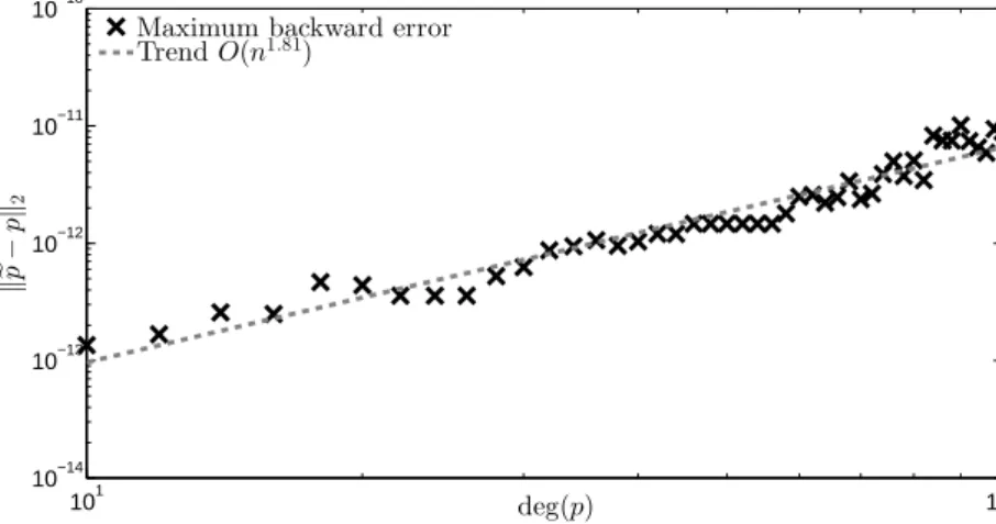
polynomial is fixed to 1. Writingǫ=nτu, whereuis the unit roundoff, notice that (3.1) predicts an upper boundO(n3+τ). To examine the tightness of this bound, for eachn= 10,12,14, . . . ,100, we generate 100 random degree-npolynomials with 2-norm equal to 1. The coefficients of these polynomials are generated via the Matlab commandsp=randn(n)andp=p/norm(p). Then, for each polynomial we compute the backward errorkpe−pk2 when its roots are computed via the eigenvalues of its
2 3 4 5 6 7 8 9 10 −12 −10 −8 −6 −4 −2 0 2 4 6 kpk2 k e p − p k2
Maximum backward error TrendO(kpk2
2)
Figure 1. Maximum backward errors obtained for each of the 9 samples of 100 random degree-10 polynomials with fixed 2-norm equal to 10k, when their roots are computed as the eigenvalues of their colleague matrices.
In Figure 2 we plot the maximum backward error obtained for each of the 46 samples of 100 random polynomials against the degree of the polynomials. In addi-tion, we also compute a linear fitting for the logarithms of the maximum backward errors to get the asymptotic dependence withn. As can be seen in Figure 2, these backward errors behave liken1.81, which means that our bound (which accounts for the worst case scenario) is overestimating the polynomial backward errors in these cases. 101 102 10−14 10−13 10−12 10−11 10−10 deg(p) k e p − p k2
Maximum backward error TrendO(n1.81)
Figure 2. Maximum backward errors obtained for each of the 46 samples of 100 random degree-n polynomials with fixed 2-norm equal to 1, when their roots are computed as the eigenvalues of their colleague matrices.
4. Conclusions
In this paper, we have analyzed the backward stability of a Chebyshev-basis polynomial rootfinder (or matrix polynomial eigensolver) based on the solution of the standard eigenvalue problem for the corresponding colleague matrix. More precisely, given a monic scalar polynomial in the Chebyshev basis p(x), we have proved that if the roots of p(x) are computed as the eigenvalues of a colleague matrix using a backward stable eigenvalue algorithm, like the QR algorithm, then the computed roots are the exact roots of a monic polynomial in the Chebyshev basispe(x) such that
kep−pk2
kpk2
=O(u)kpk2,
Similarly, if the eigenvalues of a monic matrix polynomial in the Chebyshev basis are computed as the eigenvalues of a block colleague matrix using a backward stable eigenvalue algorithm, then the computed eigenvalues are the exact eigenvalues of a monic matrix polynomial in the Chebyshev basisPe(x) such that
kPe−PkF kPkF
=O(u)kPkF,
These backward error analysis show that these methods are backward stable when the normskpk2 andkPkF are moderate.
5. Acknowledgements
We would like to thank two anonymous referees for their careful reading of the manuscript that lead to an improved presentation. We are also grateful to Froil´an Dopico for pointing out a subtlety in our original proof of Corollary 2.8; following his observation, we have filled this gap.
Appendix A. Proof of Theorem 2.1
In this section we present the proof of Theorem 2.1, that is, given the Clen-shaw shift Hn−k(x) associated with the matrix polynomialP(x) in (1.2), and the Chebyshev polynomialTn−i(x), we show that
(A.1) Tn−i(x)Hn−k(x) =Qik(x) +rik(x)P(x),
for some scalar polynomialrik(x), whereQik(x) is the matrix polynomial of degree less than or equal ton−1 in (2.4)–(2.7). Moreover, we show that the decomposition (A.1) is unique.
Along the proof, quite often products of two of Chebyshev polynomials will occur. For this reason, the following formula [1, Chapter 22] is of fundamental importance here:
The first step is to expand the Clenshaw shiftsHk(x), fork= 0,1, . . . , n−1, in the Chebyshev basis. We will prove
Hk(x) = k−1 X ℓ=0 2ΓℓTk−ℓ(x) + ΓkT0(x), fork= 0,1, . . . , n−2, and (A.3) Hn−1(x) = nX−2 ℓ=0 ΓℓTn−1−ℓ(x) + 1 2Γn−1T0(x), (A.4)
where Γℓ is defined in (2.3). The proof proceeds by induction onk. From (2.1) we getH0(x) = 2Ip= Γ0T0(x) and H1(x) = 4Ipx+ 2An−1= 2Γ0T1(x) + Γ1T0(x), so
the result is true for k = 0 and k = 1. Then, assume that the result is true for
H0(x), H1(x), . . . , Hk−1(x), with 2 ≤k ≤n−2. Using the induction hypothesis,
together with (2.1), we have
Hk(x) =2xHk−1(x)−Hk−2(x) + 2An−k =2x k−2 X ℓ=0 2ΓlTk−1−ℓ(x) + Γk−1T0(x) ! − k−3 X ℓ=0 2ΓℓTk−2−ℓ(x)−Γk−2T0(x)+ 2An−k.
Using T0(x) = 1, T1(x) = x, and (A.2) with m= 1 andn=k, from the previous
equation we get Hk(x) = k−2 X ℓ=0 2Γℓ(Tk−ℓ(x) +Tk−2−ℓ(x)) + 2Γk−1T1(x) − k−3 X ℓ=0 2ΓℓTk−2−ℓ(x)−Γk−2T0(x) + 2An−kT0(x) = k−2 X ℓ=0 2ΓℓTk−ℓ(x) + 2Γk−2T0(x) + 2Γk−1T1(x)−Γk−2T0(x) + 2An−kT0(x) = k−1 X ℓ=0 2ΓℓTk−ℓ(x) + (Γk−2+ 2An−k)T0(x) = k−1 X ℓ=0 2ΓℓTk−ℓ(x) + ΓkT0(x),
where in the last equality we have used Γk−2+ 2An−k = Γk. Therefore, the result is also true forHk(x). Finally, the proof that (A.4) holds is similar to the previous one, but starting with Hn−1(x) = xHn−2(x)−Hn−3(x)/2 +A1, so we omit the
details.
Now we proceed to show that (A.1) holds withQik(x) as in (2.4)–(2.7). In order to do that, we will proceed in certain order. To help the reader to follow the steps, we depict all the possible products Tn−i(x)Hn−k(x) for n = 10 in the following 10×10 grid.
Ti(x) Hk(x) 0 1 2 3 4 5 6 7 8 9 0 1 2 3 4 5 6 7 8 9 1 2 3 3 3 3 3 3 3 1 2 3 3 3 3 3 3 1 2 3 3 3 3 3 1 2 3 3 3 3 1 2 3 3 3 1 2 3 3 1 2 3 1 2 1
The vertices with triangular shape in the previous grid represent the cases in which the degree ofTn−i(x)Hn−k(x) does not exceedn−1, that is, wheni≥n−k+1. In this case, the polynomialQik(x) coincide withTn−i(x)Hn−k(x), so we just need to expandTn−i(x)Hn−k(x) in the Chebyshev basis. Indeed, wheni=nandk= 1, from (A.4), we have
T0(x)Hn−1(x) =Hn−1(x) = nX−2 ℓ=0 ΓℓTn−1−ℓ(x) + 1 2Γn−1T0(x), and whenn−1≥i≥n−k+ 1, from (A.2) and (A.3), we have
Tn−i(x)Hn−k(x) = n−Xk−1 ℓ=0 2ΓℓTn−i(x)Tn−k−ℓ(x) + Γn−kTn−i(x)T0(x) = n−Xk−1 ℓ=0 Γℓ(T2n−i−k−ℓ(x) +T|k+ℓ−i|(x)) + Γn−kTn−i(x).
As can be checked, the two previous equations correspond to (2.4) and (2.5), re-spectively.
Next, we consider the productsTn−i(x)Hn−k(x) withi < n−k+ 1, represented in the grid by vertices with circular shape. This case is much more involved, since the degree ofTn−i(x)Hn−k(x) is larger than or equal ton. We will prove that (A.1) holds, withQik(x) as in (2.4)–(2.7), each diagonal in the grid at a time (from left to right), showing that each productTn−i(x)Hn−k(x) can be computed using, at most, a product represented by a vertex in the same diagonal and two products represented by vertices in the diagonal on its left.
The first step is to consider the productsTk(x)Hn−k(x), fork= 1,2, . . . , n−1, that is, products represented by the diagonal with white circular vertices in the grid. We show that Theorem 2.1 holds for those products from top to bottom. We start with the white circular vertex labeled with 1 in the grid, that is, with the
productT1(x)Hn−1(x). From (2.2) and (A.3), together withT1(x) =x, we have T1(x)Hn−1(x) =xHn−1(x) = 1 2Hn−2(x)−A0T0(x) +· · · = nX−3 ℓ=0 ΓℓTn−2−ℓ(x) +1 2Γn−2T0(x)−A0T0(x) +· · ·,
where the dots correspond to something of the form r(x)P(x), with r(x) a scalar polynomial. As can be easily checked, the previous equation corresponds to (2.7) withi=n−1.
Then, we consider the white circular vertex labeled with 2 in the grid, that is, the productT2(x)Hn−2(x). From (1.1) and (2.1), we have
Hn−2(x)T2(x) =Hn−2(x) (2xT1(x)−T0(x)) = 2xT1(x)Hn−2(x)−T0(x)Hn−2(x)
=T1(x) (2Hn−1(x) +Hn−3(x)−2A1)−T0(x)Hn−2(x)
= 2T1(x)Hn−1(x) +T1(x)Hn−3(x)−T0(x)Hn−2(x)−2A1T1(x).
As can be seen from the previous equation, the product Hn−2(x)T2(x) may be
computed from products represented by two triangular vertices: T1(x)Hn−3(x) and T0(x)Hn−2(x), and the productT1(x)Hn−1(x). Then, using (A.3), (A.4), and the
result previously obtained forT1(x)Hn−1(x), we get
T2(x)Hn−2(x) =
nX−4
ℓ=0
Γℓ(Tn−2−ℓ(x) +T|ℓ+4−n|(x))+ Γn−3T1(x)−2A0T0(x)−2A1T1(x) +· · ·,
where the dots correspond to something of the form r(x)P(x), with r(x) a scalar polynomial. The previous equation corresponds to (2.6) withi=n−2 andk= 2. Finally, we consider the white circular vertices labeled with 3, that is, the prod-uctsTk(x)Hn−k(x), fork= 3,4, . . . , n. From (1.1) and (2.1), we have
Tk(x)Hn−k(x) =(2xTk−1(x)−Tk−2(x))Hn−k(x) =2xTk−1(x)Hn−k(x)−Tk−2(x)Hn−k(x)
=Tk−1(x)(Hn−k+1(x) +Hn−k−1(x)−2Ak−1)−Tk−2(x)Hn−k(x) =Tk−1(x)Hn−k+1(x) +Tk−1(x)Hn−k−1(x)−Tk−2(x)Hn−k(x)
−2Ak−1Tk−1(x).
As can be seen from the previous equation,Tk(x)Hn−k(x) may be computed from
Tk−1(x)Hn−k−1(x) andTk−2(x)Hn−k(x), represented in the grid by triangular ver-tices, andTk−1(x)Hn−k+1(x), represented in the grid by the white circular vertex
above the white circular vertex corresponding to Tk(x)Hn−k(x). Since we have previously seen that Theorem 2.1 holds forT1(x)Hn−1(x) and T2(x)Hn−2(x), and
for products represented by triangular vertices, this shows how to prove induc-tively (from top to bottom) that Theorem 2.1 holds for products represented by white circular vertices labeled with 3. Indeed, assuming that the result holds for
Tk−1(x)Hn−k+1(x) and using (2.4), we get Tk(x)Hn−k(x) =Tk−1(x)Hn−k−1+ k X r=2 (−2Ak−r)Tk−r(x)− 2Ak−1Tk−1(x) +· · ·= n−Xk−2 ℓ=0 Γℓ(Tn−2−ℓ(x) +T|ℓ+2k−n|(x))+ Γn−k−1Tk−1(x) + k X r=1 (−2Ak−r)Tk−r(x) +· · · ,
where the dots correspond to something of the form r(x)P(x), with r(x) a scalar polynomial. It is immediate to check that the previous equation corresponds to (2.6) wheni=n−k.
The second step is to consider the productsTk+1(x)Hn−k(x), fork= 2,3, . . . , n− 2, that is, the diagonal with black circular vertices in the grid. This step is very similar to the previous one, so we will only sketch the main ideas. We have to distinguish the casesk= 2, k= 3 andk >3. Whenk= 2, using (1.1), (2.1) and (2.2), it may be proved
T2(x)Hn−1(x) =T1(x)Hn−2(x)−T0(x)Hn−1(x)−2A0T1(x) +· · ·,
where the dots correspond to something of the form r(x)P(x), with r(x) a scalar polynomial. The previous equation shows that T2(x)Hn−1(x) may be computed
from two products represented by triangular vertices in the grid: T1(x)Hn−2(x) and T0(x)Hn−1(x). Since we have seen that Theorem 2.1 holds for products represented
by triangular vertices, it may be proved that (2.7) holds forT2(x)Hn−1(x).
Then, from (1.1) and (2.1), it may be proved that, whenk= 2,
T3(x)Hn−2(x) = 2T2(x)Hn−1(x) +T2(x)Hn−3(x)−2A1T2(x),
and, whenk >3,
Tk+1(x)Hn−k(x) =Tk(x)Hn−k+1(x) +Tk(x)Hn−k−1(x)− Tk−1(x)Hn−k(x)−2Ak−1Tk(x).
These two equations show thatTk+1(x)Hn−k(x) may be computed from two prod-ucts represented by triangular vertices, and the product represented by the black circular vertex above the black circular vertex corresponding to Tk+1(x)Hn−k(x). Assuming that Theorem 2.1 holds forT2(x)Hn−1(x), the previous observation shows
how to prove inductively (from top to bottom) that Theorem 2.1 holds for products corresponding to black circular vertices labeled with 2 and 3.
Now, we address the products represented by circular vertices colored with differ-ent shades of grey, that is, the products Tk+r−1(x)Hn−k(x), forr= 3,4, . . . , n−2 and k = 1,2, . . . , n−1−r. We will show that Theorem 2.1 holds for products represented by vertices in the same diagonal (same shade of grey) assuming that it holds for products represented by (non-triangular) vertices in the diagonal on its left. Since we have previously proved that Theorem 2.1 holds for products repre-sented by the white and black diagonals, this will imply that Theorem 2.1 holds for all products represented by grey vertices. For each grey diagonal, we have to distinguish the products represented by vertices labeled with 1, 2, and 3.
First, we consider the productTr(x)Hn−1(x), withr≥3, represented by a grey
vertex labeled with 1. From (1.1) and (2.2), we get
Tr(x)Hn−1(x) =(2xTr−1(x)−Tr−2(x))Hn−1(x) = 2xTr−1(x)Hn−1(x)− Tr−2(x)Hn−1(x)
=Tr−1(x)Hn−2(x)−Tr−2(x)Hn−1(x)−2A0Tr−1(x) +· · ·,
where the dots correspond to something of the form r(x)P(x), with r(x) a scalar polynomial. The previous equation shows that Tr(x)Hn−1(x) may be computed
from two products represented by vertices in the diagonal on its left: Tr−1(x)Hn−2(x)
and Tr−2(x)Hn−1(x). Assuming that (2.6) and (2.7) hold for those products, we
have Tr−1(x)Hn−2(x) = n−Xr−1 ℓ=0 Γℓ Tn−r+1−ℓ(x) +T|ℓ−n+r+1|(x) + Γn−rT1(x) − r−2 X ℓ=1 ℓ+1 X s=1 2Aℓ+1−sT|r−ℓ−s|(x) +· · ·, and Tr−2(x)Hn−1(x) = nX−r ℓ=0 ΓℓTn−r+1−ℓ(x) +1 2Γn−r+1T0(x)− r−2 X ℓ=1 ℓ X s=1 Aℓ−sT|r−ℓ−s−1|(x) +· · ·,
where the dots correspond to something of the form r(x)P(x), with r(x) a scalar polynomial. Using n−Xr−1 ℓ=0 Γℓ Tn−r+1−ℓ(x) +T|ℓ−n+r+1|(x) + Γn−rT1(x)− n−r X ℓ=0 ΓℓTn−r+1−ℓ(x) −12Γn−r+1T0(x) = n−Xr−2 ℓ=0 ΓℓTn−r−1−ℓ(x) + 1 2Γn−r−1T0(x)−Ar−1T0(x), where we have used (Γn−r+1−Γn−r−1)/2 =Ar−1, and
− r−2 X ℓ=1 ℓ+1 X s=1 2Aℓ+1−sT|r−ℓ−s|(x) + r−2 X ℓ=1 ℓ X s=1 Aℓ−sT|r−ℓ−s−1|(x) =− r−2 X ℓ=1 ℓ+1 X s=1 Aℓ+1−sT|r−ℓ−s|(x)− r−2 X ℓ=1 AℓT|r−ℓ−1|(x) =− r−2 X ℓ=1 ℓ+1 X s=1 Aℓ+1−sT|r−ℓ−s|(x)− r X s=1 Ar−sT|s−1|(x) +Ar−1T0(x) +A0Tr−1(x) =− r−1 X ℓ=0 ℓ+1 X s=1 Aℓ+1−sT|r−ℓ−s|(x) +Ar−1T0(x) + 2A0Tr−1(x) =− r X ℓ=1 ℓ X s=1 Aℓ−sT|r+1−ℓ−s|(x) +Ar−1T0(x) + 2A0Tr−1(x),
we get Tr−1(x)Hn−2(x) = n−Xr−2 ℓ=0 ΓℓTn−r−1−ℓ(x) + 1 2Γn−r−1T0(x)− r X ℓ=1 ℓ X s=1 2Aℓ−sT|r+1−ℓ−s|(x) +· · ·,
where the dots correspond to something of the form r(x)P(x), with r(x) a scalar polynomial. As can be checked, the previous equation corresponds to (2.7) with
k= 1 and i=n−r.
The proof that Theorem 2.1 holds for products represented by grey vertices labeled with 2 is very similar to the previous one, so we omit it.
Finally, consider a productTn−i(x)Hn−k(x) represented by a grey vertex labeled with 3. From (1.1) and (2.1), we have
Tn−i(x)Hn−k(x) =(2xTn−i−1(x)−Tn−i−2(x))Hn−k(x) =Tn−i−1(x)Hn−k+1(x)
+Tn−i−1(x)Hn−k−1(x)−Tn−i−2(x)Hn−k(x)−2Ak−1Tn−i−1(x)
The previous equation shows that Tn−i(x)Hn−k(x) may be computed from two products represented by (non-triangular) vertices in the diagonal on its left:
Tn−i−1(x)Hn−k−1(x) andTn−i−2(x)Hn−k(x), and a product represented by a ver-tex in the same diagonal, above the verver-tex corresponding toTn−i(x)Hn−k(x), that is, the productTn−i−1(x)Hn−k+1(x). This observation shows how to prove
induc-tively (from top to bottom) that Theorem 2.1 holds for the grey vertices labeled with 3 in the same diagonal. Assuming that (2.6) holds for Tn−i−1(x)Hn−k−1(x), Tn−i−2(x)Hn−k(x) andTn−i−2(x)Hn−k(x), and using Γi+1−Γi−1= 2An−i−1,
i−1 X ℓ=0 Γℓ(Ti+k−2−ℓ(x) +T|k+ℓ−i−2|(x)) + ΓiTk−2(x)+ i−1 X ℓ=0 Γℓ(Ti+k−ℓ(x) +T|k+ℓ−i|(x)) + ΓiTk(x)− i X ℓ=0 Γℓ(Ti+k−ℓ(x) +T|k+ℓ−i−2|(x))−Γi+1Tk−1(x) = i−2 X ℓ=0 Γℓ(Ti+k−2−ℓ(x) +T|k+ℓ−i|(x)) + Γi−1Tk−1(x)−2An−i−1Tk−1, and − n−Xk+1−i ℓ=1 k−X2+ℓ r=1 2Ak−2+ℓ−rT|n−i−ℓ−r|(x)− n−Xk−1−i ℓ=1 k+ℓ X r=1 2Ak+ℓ−rT|n−i−ℓ−r|(x) + n−Xk−1−i ℓ=1 k−X1+ℓ r=1 2Ak−1+ℓ−rT|n−i−1−ℓ−r|(x) =− n−Xk+1−i ℓ=1 k−X1+ℓ r=1 2Ak−1+ℓ−rT|n−i+1−ℓ−r|(x) + 2Ak−1Tn−i−1(x) + 2An−i−1Tk−1(x).
we get Tn−i(x)Hn−k(x) =Tn−i−1(x)Hn−k+1(x) +Tn−i−1(x)Hn−k−1(x)− Tn−i−2(x)Hn−k(x)−2Ak−1Tn−i−1(x) = i−2 X ℓ=0 Γℓ(Ti+k−2−ℓ(x) +T|k+ℓ−i|(x)) + Γi−1Tk−1(x)− n−Xk+1−i ℓ=1 k−X1+ℓ r=1 2Ak−1+ℓ−rT|n−i+1−ℓ−r|(x) +· · · ,
where the dots correspond to something of the form r(x)P(x), with r(x) a scalar polynomial, which shows that (2.6) holds also forTn−i(x)Hn−k(x).
The final step of the proof consists in proving the uniqueness ofrik(x) andQik(x) in (A.1). For this purpose, assume that there exist two scalar polynomials rik(x) anderik(x), and two matrix polynomialsQik(x) andQeik(x) of degree at mostn−1 such that Tn−i(x)Hn−k(x) = Qik(x) +rik(x)P(x) =Qeik(x) +reik(x)P(x). Then,
Qik(x)−Qeik(x) = (erik(x)−rik(x))P(x) is a matrix polynomial of degree at most
n−1, but, if rik(x) 6= erik(x), the matrix polynomial (erik(x)−rik(x))P(x) has degree larger than or equal ton, hencerik(x) =erik(x) andQik(x) =Qeik(x).
References
1. M. Abramowitz and I. A. Stegun, Handbook of Mathematical Functions: with Formulas, Graphs, and Mathematical Tables. Number 55. Courier Dover Publications, 1972.
2. A. Amiraslami, R. M. Corless, and P. Lancaster,Linearization of matrix polynomials expressed in polynomial bases. IMA. J. Numer. Anal.29(2009), no. 1, 141–157.
3. V. I. Arnold,On matrices depending on parameters, Russian Matehmatical Surveys26(1971), no. 2, 29–43.
4. S. Barnett,Polynomials and Linear Control Systems. Marcel Dekker Inc., 1983.
5. S. Barnett.Leverrier’s Algorithm for Orthogonal Polynomial Bases. Linear Algebra Appl.236 (1996), 245–263, 1996.
6. C. W. Clenshaw,A note on the summation of Chebyshev series. Math. Comp.9(1955), 118– 120.
7. F. De Ter´an, F. M. Dopico, and D. S. Mackey, Fiedler companion linearizations and the recovery of minimal indices. SIAM J. Matrix Anal. Appl.31(2009/2010), no. 4, 2181–2204. 8. F. De Ter´an, F. M. Dopico, and J. P´erez,Backward stability of polynomial root-finding using
Fiedler companion matrices. IMA J. Numer. Anal., in press, DOI 10.1093/imanum/dru057. 9. A. Edelman and H. Murakami,Polynomial roots from companion matrix eigenvalues. Math.
Comp.64(1995), 763–776.
10. C. Effenberger and D. Kressner,Chebyshev interpolation for nonlinear eigenvalue problems. BIT52(2012), 933–951.
11. I. J. Good,The colleague matrix, a Chebyshev analogue of the companion matrix. Q. J. Math. 12(1961), 61–68.
12. P. Lancaster and M. Tismenetsky,The Theory of Matrices.Second Ed., Academic Press, San Diego, 1985.
13. P. W. Lawrence and R. M. Corless, Stability of rootfinding for barycentric Lagrange inter-polants. Numer. Algorithms65(2014), 447–464.
14. P. W. Lawrence, M. Van Barel, and P. Van Dooren, Structured backward error analysis of polynomial eigenvalue problems solved by linearizations. Preprint, submitted.
15. D. Lemmonier and P. Van Dooren,Optimal scaling of companion pencils for the QZ-algorithm. Proceedings SIAM Appl. Lin. Alg. Conference, Paper CP7-4, 2003
16. D. Lemmonier and P. Van Dooren,Optimal scaling of block companion pencils. Proceedings of the International Symposium on Mathematical Theory of Networks and Systems, Leuven, Belgium, 2004.
17. J. Maroulas and S. Barnett,Polynomials with respect to a general basis. I. Theory. J. Math. Anal. Appl.72(1979), no. 1, 177–194.
18. Y. Nakatsukasa and V. Noferini,On the stability of computing polynomial roots via confederate linearizations. To appear in Math. Comp.
19. Y. Nakatsukasa, V. Noferini, and A. Townsend, Vector spaces of linearizations for matrix polynomials: a bivariate polynomial approach. Preprint, submitted.
20. V. Noferini and F. Poloni,Duality of matrix pencils, Wong chains and linearizations. Linear Algebra Appl.471(2015), 730–767.
21. B. N. Parlett and C. Reinsch, Balancing a matrix for calculation of eigenvalues and eigen-vectors. Numer. Math.13(1963), 293–304.
22. G. Peters and J. H. Wilkinson,Practical problems arising in the solution of polynomial equa-tions. J. Inst. Maths. Appl.8(1971), 16–35.
23. L. N. Trefethen,Approximation theory and approximation practice. SIAM, 2013.
24. L. N. Trefethen et al, Chebfun Version 5. The Chebfun Development Team, 2014.
http://www.maths.ox.ac.uk/chebfun/.
25. K. -C. Toh and L. N. Trefethen,Pseudozeros of polynomials and pseudospectra of companion matrices. Numer. Math.68(1994), 403–425.
26. J. H. Wilkinson, Rounding Errors in Algebraic Processes. Prentice-Hall, Englewood Cliffs, 1963.
27. J. H. Wilkinson,The Algebraic Eigenvalue Problem. Clarendon Press, Oxford, 1965.
School of Mathematics, The University of Manchester, Manchester, England, M13 9PL
E-mail address: [email protected]
School of Mathematics, The University of Manchester, Manchester, England, M13 9PL