(will be inserted by the editor)
Maximum Margin Hashing with Supervised Information
Haichuan Yang, Xiao Bai, Yanzhen Liu, Yanyang Wang, Lu Bai, Jun Zhou, Wenzhong Tang
Received: date / Accepted: date
Abstract Binary code is a kind of special representation of data. With the binary format, hashing framework can be built and a large amount of data can be indexed to achieve fast research and retrieval. Many supervised hash-ing approaches learn hash functions from data with supervised information to retrieve semantically similar samples. This kind of supervised information can be generated from external data other than pixels. Conventional supervised
H. Yang
School of Computer Science and Engineering, Beihang University, 37 Xueyuan Road, Haid-ian District, Beijing, China
X. Bai
School of Computer Science and Engineering, Beihang University, 37 Xueyuan Road, Haid-ian District, Beijing, China
E-mail: [email protected] Y. Liu
School of Computer Science and Engineering, Beihang University, 37 Xueyuan Road, Haid-ian District, Beijing, China
Y. Wang
School of Aeronautic Science and Engineering, Beihang University, 37 Xueyuan Road, Haid-ian District, Beijing, China
E-mail: [email protected] L. Bai
School of Information, Central University of Finance and Economics, 100081, Beijing, China J. Zhou
School of Information and Communication Technology, Griffith University, Nathan, QLD 4111, Australia
W. Tang
School of Computer Science and Engineering, Beihang University, 37 Xueyuan Road, Haid-ian District, Beijing, China
hashing methods assume a fixed relationship between the Hamming distance and the similar (dissimilar) labels. This assumption leads to too rigid require-ment in learning and makes the similar and dissimilar pairs not distinguish-able. In this paper, we adopt a large margin principle and define a Hamming margin to formulate such relationship. At the same time, inspired by support vector machine which achieves strong generalization capability by maximiz-ing the margin of its decision surface, we propose a binary hash function in the same manner. A loss function is constructed corresponding to these two kinds of margins and is minimized by a block coordinate descent method. The experiments show that our method can achieve better performance than the state-of-the-art hashing methods.
1 Introduction
Nearest neighbor (NN) search plays an important role in machine learning and information retrieval. It can be used to recognize patterns [7] or as a procedure in other algorithms. A large number of information retrieval frameworks query the most relevant instances through NN search. However, NN search is ineffi-cient for large scale applications, and its time complexityO(n) can not meets the realtime requirement. Because of this defect, hashing was introduced [12] to retrieve the approximate nearest neighbors (ANN) by mapping the data to binary embeddings. Compared with other indexing methods, hashing needs little storage and attains constant or sublinear time complexity. Early hashing methods were proposed based on certain mathematical properties to generate hash functions without any training data. These methods are called data-independent methods, in which locality sensitive hashing (LSH) [5, 8] is the most representative example.
Using training data to learn hash functions can improve the hashing per-formance and generate compact codes [36]. This leads to the development of data-dependent hashing. Based on the training strategy, data-dependent hash-ing methods can be divided into unsupervised hashhash-ing [36, 43, 15, 11, 35, 18, 40, 10, 41, 24, 21] and supervised hashing [19, 32, 27–29, 23, 37, 42]. In addition, some methods are considered as semi-supervised hashing [34, 33] because they do not require all training data to be labeled. Severa methods can adapt to both un-supervised and un-supervised scenario by incorporating different similarities [17, 34, 25, 1] or dimensionality reduction methods [9].
Unsupervised hashing methodis the most basic prototype of this area. In fact, data-independent method,i.e.locality sensitive hashing[8] is also under the unsupervised settings. Unsupervised hashing is based on the requirement of approximate similarity search,i.e.,finding the nearest neighbors according to a given metric. The objective of unsupervised hashing is defined by certain similarity function,e.g., the Euclidean distance. Their performance is usually evaluated based on Euclidean neighbor search. K-means hashing [10] extends the idea of product quantization to using clustering methods to generate hash functions. Spherical hashing [11] uses sphere to model hash function. In [39,
0 4 8 12 16 20 24 28 32
Data with binary code -1 for h(k)
(·)
Data with binary code +1 for h(k) (·) Hyp erpl ane mar gin dH( , ) dH( , ) Decision surface of h(k) (·) ts td
Hamming margin dH(·,·) of similar pair
dH(·,·) of dissimilar pair
Simultaneously maximize their margins
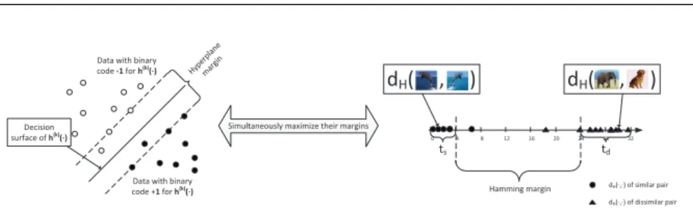
Fig. 1 Hamming margin and hyperplane margin. They are the optimization targets in our method.
38], the authors proposed a feature aggregating hashing method to achieve image copy detection on large scale data. If we can represent each image as a feature vector,e.g.,GIST feature [30], we can do efficient content based image retrieval by directly applying unsupervised hashing.
Recently, researchers also develop product quantization methods [13, 45] to get more accurate Euclidean neighbors than using hashing, sacrificing not much efficiency. However, the performance of using unsupervised indexing methods in image retrieval system largely relies on the image feature, which is usually cannot be optimally extracted. On the other hand, if we take use of the external data besides pixel information, we do not have this limitation any more.
Supervised hashingjust follows this strategy and it aims at training hash functions which output similar binary codes for data which are labeled similar. One can use many external information to label the data, e.g., the human handed annotation, the distance under other features. This kind of information is widely used in computer vision problems [44]. Therefore, supervised hashing is not only an indexing method for boosting the retrieval speed, but also can be treated as a special representation learning method [2]. Recently, by using multiple features or involving multi-view application, there are lots of hashing methods are proposed with the multimedia background [22, 14, 25, 3, 20].
This paper focuses on learning hash functions in supervised manner. Re-cently, some methods incorporate the specific representation into hashing frame-work,e.g., multimodal [42] and deep convolutional network feature [37]. How-ever, we aim at learning hash functions with any vectorized data. For super-vised hashing, the supersuper-vised information is often provided as a similar set
S and a dissimilar set D. Each set contains a number of pairs (i, j) which indicate instances i and j are similar or dissimilar. Although the supervised information can be given in other formats (e.g., class labels), they can be eas-ily transformed to this form. If there are ninstances in the training set, let
Y be an n×rmatrix whose i-th row is the binary code of thei-th instance, and dH(i, j) be the Hamming distance between the binary codes ofi and j, then the objective is thatdH(i, j) should be small for (i, j)∈ S, and dH(i, j) should be large for (i, j)∈ D. However, this objective is not definite, because it
does not define explicitly on how small (large) the Hamming distancedH(i, j) should be.
In [23], the defined objective forces the similar pairs to have the smallest Hamming distance 0 and the dissimilar pairs to have the largest Hamming dis-tancer(the code length). In [28], Norouzi and Fleet proposed a loss function with an additional parameterρ. It requires that the similar pairs have Ham-ming distance no more thanρand the dissimilar pairs have Hamming distance no less than ρ. Nevertheless, the first definition is too strict to comply with and the second one is so slack that could make the Hamming distances of the similar pairs and dissimilar pairs not discriminative. Since each hash function maps the data to a binary code in{−1,+1}, the binary classifier is suitable for the modeling. Furthermore, because support vector machine (SVM) [6] shows high generalization capability by maximizing the margin of its decision sur-face, an intrinsic idea is using the similar model as the hash function. In [43], SVM is used to train hash functions, but the binary codes and hash functions are learned in two separate stages.
In this paper, we propose a novel hashing method to overcome the problems mentioned above. To well formulate the consistency of the Hamming distance and supervised affinity between each pair (i, j), we define a Hamming margin
which equals the lower bound of dH(i0, j0) for all (i0, j0)∈ D minus the upper bound ofdH(i, j) for all (i, j)∈ S. Instead of splitting into two separate stages, our method simultaneously learns the binary codes and hash function so as to maximize the margin of the hash function. For discriminating this margin from the Hamming margin mentioned before, we refer to it as thehyperplane margin, and illustrate these two margins in Figure 1. Because our key idea is based on these two kinds of margin maximization, we name our method maximum margin hashing (MMH).
2 Formulation
The goal of our method is simultaneously maximizing the Hamming margin and the hyperplane margin. In this section, we formulate the loss functions to maximize these two margins respectively, and concatenate them into an integrated loss function.
2.1 Hamming Margin Loss
We first define two tolerance variables ts and td. As shown in Figure 1, they control the thresholds of Hamming distance of pairs inSandD. Specifically, if the code length isr, we requiredH(i, j)≤tsfor all (i, j)∈ Sandr−dH(i0, j0)≤
td for all (i0, j0)∈ D. To prevent the Hamming distances of pairs in S andD from intersecting, we force the Hamming marginr−(ts+td) to be positive,
i.e., ts+td < r. Considering this constraint may be too rigid, we adopt the soft margin concept in the proposed Hamming margin. For the instance pair
(i, j), the penalization is lij(ts, td) = ( [dH(i, j)−ts]+ for (i, j)∈ S; [(r−dH(i, j))−td]+ for (i, j)∈ D. (1)
where [α]+ is the same as max(0, α). The Hamming margin loss is defined as:
L1= (td+ts)2+η
n
X
i<j
lij(ts, td)2 (2)
whereηis a positive number for tuning the weight of the penalization. Because the supervised information is symmetric, we only count the i < j pairs in. The first term (td+ts)2 corresponds to Hamming margin maximization. The increase of tm or td will enlarge the first term and reduce the second term, and the parameterη makes a trade off between them. What should be noted is thatdH(i, j) is a function of the rows inY, and matrixY is also variables in our problem.
2.2 Hyperplane Margin Loss
As mentioned in the introduction section, we use the hyperplane based decision surface to model the hash function, so thek-th hash functionh(k)(·) is defined
as:
h(k)(xi) = sign(w(k)Txi+b(k)) (3) where w(k) and b(k) are the variables in h(k)(·), and xi is the representation vector of instance i. This definition is the same as in the kernel-based SVM. The hyperplane margin loss is analogous to the loss function used in SVM:
L2= r X k=1 (1 2kw (k)k2+C n X i=1 [1−Yik(w(k)Txi+b(k))]+) (4)
where C is a positive parameter used to penalize the violation caused by using the soft margin, Yik is the element in i-th row,k-th column ofY, and
H ={h(k)(·)}r
k=1 is the set of r hash functions. The difference between our
objective in equation (4) and the objective in SVM is that for i= 1,2, ..., n,
Yik are also variables that need to be optimized, so our objective is a more complex problem.
Finally, our integrated objective is minimizing the Hamming margin loss in equation (2) and the hyperplane margin loss in equation (4) simultaneously. We combines them as a weighted sum:
min H,Y,ts,td λL1+L2 subject to Y ∈ {−1,+1}n×r, ts, td∈ {0,1, ..., r}, ts+td < r (5)
3 Optimization
In Section 2, we have presented the objective (5). It is not differentiable because of the [·]+ operator. Moreover, it has a large number of variables including
real-valued numbers, nonnegative integers, and binary numbers. This leads to a complex and discontinuous feasible set. It is difficult to find an efficient method that can solve it directly. In this section, we propose to use the block coordinate descent (BCD) approach and enable some relaxation to get a good solution. The principle of BCD is separating the variables into several groups, and optimizing the problem with respect to each group of variables iteratively.
3.1 Optimizing with Fixed Tolerance Variables
Firstly, we assume the tolerance variables ts and td are constant, i.e., ts = ˆ
ts, td= ˆtd. Lety(k) corresponds to thek-th column ofY. Since the structure of each hash function and hash bit is the same, we group them to use the BCD. After removing the constant terms, the subproblem is:
min w(k),b(k),y(k)λ·η n X i<j lij(ˆts,ˆtd)2+ 1 2kw (k)k2+C n X i=1 [1−y(ik)(w(k)Txi+b(k))]+ (6)
Then we can iteratively optimize the subproblems with k= 1,2, ..., r untilY
converges. This is also a difficult problem, so we simplify it by using BCD again.
Fix y(k)and update w(k), b(k),i.e.,y(k) i = ˆy
(k)
i . After fixingy
(k), solving
the optimalw(k), b(k) is just the same problem in SVM:
argmin w(k),b(k) 1 2kw (k)k2+C n X i=1 [1−yˆi(k)(w(k)Txi+b(k))]+ (7)
There are many SVM solvers that can be used to solve this optimization problem. Here we use its subgradient and L-BFGS method for efficiency.
Fix w(k), b(k) and update y(k),i.e., w(k)= ˆw(k), b(k)= ˆb(k). This situa-tion is more complex. We first simplify the terms with the following proposi-tions.
Proposition 1 Let l(¯ijk)(ˆts,ˆtd) = l(d (¯k)
H (i, j); ˆts,ˆtd)denote the penalization in equation (1) between i and j excluding the k-th bit, where d(¯Hk)(i, j) is the Hamming distance excluding thek-th bit, then we have:
n X i<j lij(ˆts,ˆtd)2= n X i<j (l(¯ijk)(ˆts,ˆtd)2+ 1 2Wij(1−y (k) i y (k) j )) (8)
whereW is ann×nmatrix andWij=l(d (¯k)
H (i, j)+1; ˆts,ˆtd)2−l(d (¯k)
Proof It is obvious thatl(dH(i, j); ˆts,ˆtd)2= ( l(d(¯Hk)(i, j); ˆts,ˆtd)2+Wij·0, y (k) i =y (k) j ; l(d(¯Hk)(i, j); ˆts,ˆtd)2+Wij·1, y (k) i 6=y (k) j .
Merging these two situations into one expression, we get equation (8).
Proposition 2 Letγi= ˆw(k)Txi+ˆb(k), thenP n i=1[1−y (k) i ( ˆw(k)Txi+ˆb(k))]+ = − X |γi|<1 γiy (k) i − 1 2 X |γi|≥1 (sign(γi) +γi)y (k) i + X |γi|<1 1 +1 2 X |γi|≥1 (1 +|γi|) (9)
Proof It is easy to get the piecewise formulation that [1−y(ik)( ˆw(k)Tx i+ ˆb(k))] += 1 +|γi| for|γi|<1, andy (k) i sign(γi) =−1; 1− |γi| for|γi|<1, andy (k) i sign(γi) = 1; 1 +|γi| for|γi| ≥1, andy (k) i sign(γi) =−1; 0 for|γi| ≥1, andy (k) i sign(γi) = 1. Merge it as: ( 1−sign(γi)y (k) i |γi| for|γi|<1; 1 2(1 +|γi|)(1−sign(γi)y (k) i ) for|γi| ≥1. Using the above equation for summing, we get the equation (9).
With the Propositions 1, 2 and the fact thatl(¯ijk)(ˆts,ˆtd) andγiare constants here, the subproblem defined in equation (6) with fixedw(k), b(k)becomes:
min y(k){λ·η n X i<j 1 2Wij(1−y (k) i y (k) j ) +C(− X |γi|<1 γiy (k) i −1 2 X |γi|≥1 (sign(γi) +γi)y (k) i )}
Furthermore, we can represent this problem as an unconstrained binary quadratic programming (BQP): min y(k) 1 2y (k)TLy(k)+aTy(k) subject to y(k)∈ {−1,+1}n (10)
with then×nmatrixLandndimensional vectora: L=1 2λ·η(Diag(We)−W), ai= ( −Cγi for|γi|<1; −C(sign(γi) +γi)/2 for|γi| ≥1. (11)
where Diag(We) is a diagonal matrix with thei-th diagonal element being the sum of thei-th row inW.
Although equation (10) has a very compact form, it is an NP-hard problem [31]. Some relaxation solutions have been proposed for it [31]. To optimize our integrated objective, we need to solve this kind of BQP many times, so the efficiency of the BQP solver is crucial. In this paper, we use a simple approximation: min z 1 2tanh(z T)Ltanh(z) +aTtanh(z) (12) where tanh(·) is used as a smooth approximation of sign(·).
Equation (12) is an unconstrained optimization problem, so we use its gra-dient and the L-BFGS method to optimize it. The binary variables can be obtained by sign(z∗), wherez∗ is the minimum point. Our solution iteratively updatesw(k), b(k) and{y(k)
i }ni=1 until they converge, then goes on to the
op-timization with the (k+ 1)-th hash function and bit.
3.2 Updating the Tolerance Variables
Following the above procedures, we can getHandY in equation (5) with fixed
tsandtd. Here we use the BCD principle again to update these two variables. If the binary code matrixY is given, the Hamming distances are constant,
i.e., dH(i, j) = ˆdH(i, j). It should be noted that the variables ts and td only appear inL1, so the subproblem becomes nonlinear integer programming:
min ts,td (td+ts)2+η( X (i,j)∈S [ ˆdH(i, j)−ts]2++ X (i,j)∈D [r−dˆH(i, j)−td]2+) subject to ts, td∈ {0,1, ..., r}, ts+td < r (13)
The objective function is a nonnegative weighted sum of several convex func-tions, so it is also a convex function. However, its feasible set is a triangular lattice which is discrete. Here we propose a steepest direction search method which is analogous to gradient descent, but is applicable to discrete optimiza-tion.
Let f denote the objective function in (13), the steepest direction search method consists of following steps:
1. Select four points (ts±1, td) and (ts, td±1), and choose the feasible points (maintain the constraint in equation (13)) in them as candidates;
2. Compute the value of f on the candidates, and choose the minimal point (t∗s, t∗d);
3. Iff(t∗
s, t∗d)< f(ts, td), update (ts, td) with (t∗s, t∗d) and go to step 1. Other-wise stop and return (ts, td).
With the above procedure, we can get the point (ts, td) which has the minimal
f in its adjacencies (ts±1, td) and (ts, td±1). Furthermore, because of the con-vexity of functionf, we havef(ts, td)≤f(ts±t, td) andf(ts, td)≤f(ts, td±t), wheretis an arbitrary integer. Although this is not a global optimal solution, it is usually good enough for our problem. After updatingts, td, we can opti-mize H, Y according to Section 3.1. Finally, the whole procedure for solving our objective in equation (5) is shown in Algorithm 1.
Algorithm 1: Maximum Margin Hashing
Data: Representation vectors{xi}ni=1, similar setS, dissimilar setD, code lengthr
and parametersλ, η, C.
Result: Hash function setH.
Initializets, tdand binary code matrixY ∈ {−1,+1}n×r.
repeat // Iteration 1
k←1.
repeat // Iteration 2
Construct matrixL∈Rn×nas equation (11);
repeat // Iteration 3
Construct vectora∈Rnas equation (11) or initiateaas0in the first
round;
Solve the local minimaz∗of the unconstrained problem (12);
y(ik)←sign(z∗
i), fori= 1,2,3, ..., n;
Solve the optimalw(k), b(k)of the SVM problem (7) with datax
iand labelsy(ik); until{yi(k)}n i=1,w(k), b(k) are converged; Yik←y (k) i , i= 1,2,3, ..., n; k←k+ 1; if k > rthen k←1 end untilY is converged;
Updatets, tdaccording to the steepest direction search in Section 3.2.
untilts, tdare converged;
H ← {h(k)(·)}r
k=1. // h(k)(x) =sign(w(k)Tx+b(k))
4 Implementation Details
Initialization. Some variables in Algorithm 1 need to be initialized. At the beginning of the whole process, we initialize ts = 0, td = 0 so as to start with the largest Hamming margin. The matrix Y is initialized with random
projections of {xi}ni=1. In the first round, since w
(k), b(k) are not given, we
can initiatea=0. To proceed the L-BFGS method for equation (12), we also need an initial pointz. Here we set it as√n·uwhere uis the eigenvector of
Lcorresponding to the least eigenvalue and aTu<0. At the end of iteration 1, we use the previoustsandtd to start the steepest direction search.
Convergency. In Algorithm 1, all stop criteria are the variables to be converged. For the BCD method, the value of objective function will decrease after each iteration if the global minima of the subproblem is attained. In our method, we usually can not get the global minima, but we can guarantee that the value of objective function does not increase after each iteration. In practice, if the solved variables for the subproblem will increase the overall loss, we do not update the corresponding variables. Therefore, the variables will be converged when the loss is small enough.
Parameters. The main parameters in our method are the tradeoff param-etersλ, ηandC.λcontrols the balance betweenL1andL2, andCis similar to
the soft margin weight in SVM. As in many algorithms, these parameters need to be tuned on different datasets. In our experiments, we setη =n(n−1)/2, and tunedλandC.
5 Experiments
5.1 Experiments Set up
Datasets. We evaluated the performance of the proposed method on two popular image datasets, MNIST1, CIFAR-10 [16] and one multi-modal dataset Wiki2. They are widely used in hashing evaluations [17, 34, 27, 28, 33, 23, 9].
MNIST dataset consists of 70,000 28×28 gray scale images of handwritten digits. This dataset has 10 classes corresponding to the 0∼9 digits, with all images being labeled. The digit in each image is well aligned, so the pixel values can be treated as a 784-dimension feature vector. Because a large portion of pixels are clean background pixels in each image, each feature vector is sparse. CIFAR-10 dataset consists of 60,000 32×32 color images in 10 classes in-cluding airplane, automobile, bird, cat, deer, dog, frog, horse, ship, and truck. Each class has 6,000 images. For CIFAR-10, the images are too small to ex-tract adequate local features such as SIFT [26]. Since they have the same size, we use a 512-dimensional GIST descriptor [30] to represent each image.
Wiki dataset contains images and texts from Wikipedia. The size of whole dataset is 2,886, and every sample is a image-text pair. In our experiment, we use the 128-dimensional SIFT based bag-of-visual word representation for the image, and 10-dimensional topic vector for the text content.
For the two image datasets, the image label is actually the supervised information which can be seen as the external data for pixel data of images. For dataset Wiki, we compute the Euclidean distance between the texts’ features
1 http://yann.lecun.com/exdb/mnist/
0 0.2 0.4 0.6 0.8 1 0.1 0.2 0.3 0.4 0.5 0.6 0.7 0.8 0.9 1 Recall Precision MMH−kernel MMH−linear KSH MLH BRE S3PLH CCA−ITQ (a) 16 bits 0 0.2 0.4 0.6 0.8 1 0.1 0.2 0.3 0.4 0.5 0.6 0.7 0.8 0.9 1 Recall Precision MMH−kernel MMH−linear KSH MLH BRE S3PLH CCA−ITQ (b) 32 bits 0 0.2 0.4 0.6 0.8 1 0.1 0.2 0.3 0.4 0.5 0.6 0.7 0.8 0.9 1 Recall Precision MMH−kernel MMH−linear KSH MLH BRE S3PLH CCA−ITQ (c) 48 bits
Fig. 2 Precision-recall curves on MNIST.
and set an threshold τ to decide whether two images are similar(< τ) or dissimilar(≥τ).
Evaluation Protocols and Baseline Methods. In the experiments, we assess the proposed maximum margin hashing (MMH) method. Each image has a single class label in MNIST and CIFAR-10. Images in the same class are considered as the semantic neighbors to each other. For fair comparison, we compare our methods with some state-of-the-art supervised hashing methods, which include kernel-based supervised hashing (KSH) [23], minimal loss hash-ing (MLH) [28], binary reconstructive embeddhash-ing (BRE) [17], semi-supervised sequential projection learning hashing (S3PLH) [34], and iterative quantiza-tion based on CCA (CCA-ITQ) [9]. In the end of the training procedure, we can learn the kernelized hash function by LIBSVM [4] with labels inY. We denote the linear version and kernelized version as linear and MMH-kernel, respectively. For the methods which use kernel-based hash functions, we adopt the same Gaussian RBF kernel exp(−kxi−xjk2/σ), whereσis set as the mean of squared Euclidean distances of the training set. For MNIST and CIFAR-10, we randomly choose 1,000 samples as the query images, and use the rest of the dataset as the target of the search, and for Wiki, the number of query is 100. For MMH,KSH,MLH, and BRE, the scale of the training set can not be too large because they are based on pairwise supervised information, we randomly choose 1,000 instances for training. S3PLH is a semi-supervised method, we choose 1,000 labeled images and take the rest images in training set as unlabeled for training. CCA-ITQ can be trained on large scale dataset since its training time is mainly dependent on the dimensionality of the data, so we randomly choose 50,000 instances for training. All the other parameters are set according to the original papers reporting these methods.
5.2 Evaluation of Retireval Performance
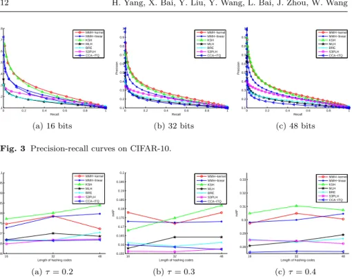
Evaluation with the Overall Measure. To demonstrate the overall per-formance, the precision-recall curves are shown in Figures 2 and 3. For the given queries, we increase the Hamming radius from 0 tor, and compute the precision and recall values of the retrieved instances, then the precision-recall
0 0.2 0.4 0.6 0.8 1 0.1 0.2 0.3 0.4 0.5 0.6 0.7 0.8 Recall Precision MMH−kernel MMH−linear KSH MLH BRE S3PLH CCA−ITQ (a) 16 bits 0 0.2 0.4 0.6 0.8 1 0.1 0.2 0.3 0.4 0.5 0.6 0.7 0.8 0.9 1 Recall Precision MMH−kernel MMH−linear KSH MLH BRE S3PLH CCA−ITQ (b) 32 bits 0 0.2 0.4 0.6 0.8 1 0.1 0.2 0.3 0.4 0.5 0.6 0.7 0.8 0.9 1 Recall Precision MMH−kernel MMH−linear KSH MLH BRE S3PLH CCA−ITQ (c) 48 bits
Fig. 3 Precision-recall curves on CIFAR-10.
16 32 48 0.06 0.065 0.07 0.075 0.08 0.085 0.09 0.095 0.1
Length of hashing codes
mAP MMH−kernel MMH−linear KSH MLH BRE S3PLH CCA−ITQ (a)τ= 0.2 16 32 48 0.155 0.16 0.165 0.17 0.175 0.18 0.185 0.19 0.195 0.2
Length of hashing codes
mAP MMH−kernel MMH−linear KSH MLH BRE S3PLH CCA−ITQ (b)τ= 0.3 16 32 48 0.28 0.29 0.3 0.31 0.32 0.33
Length of hashing codes
mAP MMH−kernel MMH−linear KSH MLH BRE S3PLH CCA−ITQ (c)τ= 0.4
Fig. 4 Mean Average Precision with different parameterτ on Wiki.
curve is plotted according to ther+ 1 points. It can be seen that our method MMH-kernel achieves the best results on both datasets, while the superiority on MNIST is more significant. Using the linear hash functions, our method MMH-linear has a lower performance compared with MMH-kernel and another kernel-based method KSH, but outperforms the others. Almost all methods get better results when using longer hash codes, except for CCA-ITQ. The reason is that CCA-ITQ is based on the Canonical Correlation Analysis which is for generating low dimensional output, so the useful information will be diluted if too long hash codes are used. For all the methods, the performances on MNIST are better than on CIFAR-10. We think this is due to the differ-ences on low level representations and the difficulty of the retrieval tasks. For dataset Wiki, we show the mean average precision (mAP) in Figure 4, which is the area under the precision-recall curve, with different value ofτ.
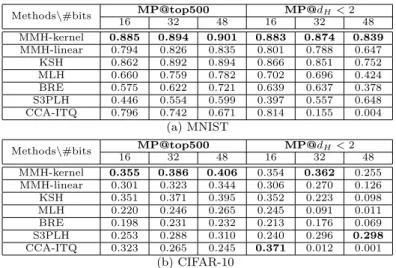
Evaluation for the Practical Usage. In practice, there are two major applications for the hash codes,i.e.Hamming ranking and hash lookup. Ham-ming ranking compares the hash code of the query with all samples in the database, which leads to linear complexity but can be efficient thanks to the efficiency of comparison between binary codes. Hash lookup retrieves samples that fall in the buckets within a given Hamming radius. In Table 1, we show the mean precisions (MP) for the top 500 Hamming neighbors (for Hamming ranking) and samples whose Hamming distances to the query is less than 2 (for hash lookup). In most situations, our method MMH-kernel has the highest
Table 1 Mean precisions and on MNIST and CIFAR-10.
Methods\#bits MP@top500 MP@dH<2
16 32 48 16 32 48 MMH-kernel 0.885 0.894 0.901 0.883 0.874 0.839 MMH-linear 0.794 0.826 0.835 0.801 0.788 0.647 KSH 0.862 0.892 0.894 0.866 0.851 0.752 MLH 0.660 0.759 0.782 0.702 0.696 0.424 BRE 0.575 0.622 0.721 0.639 0.637 0.378 S3PLH 0.446 0.554 0.599 0.397 0.557 0.648 CCA-ITQ 0.796 0.742 0.671 0.814 0.155 0.004 (a) MNIST
Methods\#bits MP@top500 MP@dH<2
16 32 48 16 32 48 MMH-kernel 0.355 0.386 0.406 0.354 0.362 0.255 MMH-linear 0.301 0.323 0.344 0.306 0.270 0.126 KSH 0.351 0.371 0.395 0.352 0.223 0.098 MLH 0.220 0.246 0.265 0.245 0.091 0.011 BRE 0.198 0.231 0.232 0.213 0.176 0.069 S3PLH 0.253 0.288 0.310 0.240 0.296 0.298 CCA-ITQ 0.323 0.265 0.245 0.371 0.012 0.001 (b) CIFAR-10
precision. When the hash code lengthris too large, the performance of hash lookup may be worse with longer codes because the hash table becomes too sparse in this situation.
Table 2 Training times (seconds) on MNIST and CIFAR-10.
Methods\#bits Training time on MNIST Training time on CIFAR-10
16 32 48 16 32 48 MMH-kernel 17.62 41.81 58.62 21.61 36.26 41.66 MMH-linear 15.44 34.21 47.08 20.15 35.33 38.41 KSH 32.07 67.61 105.6 32.95 64.98 104.84 MLH 438.1 2279 3545 465.7 2184 3476 BRE 34.29 65.96 158.1 48.58 114.4 270.4 S3PLH 18.24 35.50 53.36 9.389 18.17 28.47 CCA-ITQ 2.507 3.392 4.326 1.719 2.628 3.554
5.3 Time Efficiency Comparison
Since the specific number of iterations is not determined, the theoretical train-ing complexity of our method is not definite. In Algorithm 1, we can see there are three kinds of iterations. Usually, iteration 1 and 3 only repeat less than ten times. Iteration 2 usually repeats less than 2r times. In our implemen-tation, we limit the maximal number of iteration of solving problem 12 and 7. The elapsed time for training are shown in Tables 2. All the experiments are conducted on a PC with Core-i7 3.4GHz CPU and 16GB RAM. We can see that our methods MMH-kernel and MMH-linear consume less time than most methods, and only longer than CCA-ITQ and S3PLH whose retrieval performances are much lower.
In the indexing procedure, for the methods using linear hash function,
i.e., MMH-linear, MLH, S3PLH, and CCA-ITQ, the time complexity of each hash function isO(d), wheredis the dimensionality of data. Methods MMH-kernel, KSH, and BRE use kernelized hash function and the time complexity of Gaussian kernel is O(d), so the time complexity of their hash function is
O(µd+µ), whereµis the number of the support vectors.
6 Conclusion
In this paper, we present a supervised hashing based on two kinds of margins,
i.e. the Hamming margin and the hyperplane margin. Our Hamming margin loss is a more general definition of the requirement on the relationship between Hamming distance and the supervised labels, whereas many other methods only use a fixed Hamming margin. At the same time, we require the decision surface of hash function having a large margin to enhance the generalization capability as SVM. Experiments have shown the superiority of our approach.
7 Acknowledge
This work was supported by NSFC projects (No. 61370123 and 61503422), and the Australian Research Councils DECRA Projects funding scheme (project ID 522 DE120102948).
References
1. Bai, X., Yang, H., Zhou, J., Ren, P., Cheng, J.: Data-dependent hashing based on
p-stable distribution. Image Processing, IEEE Transactions on23(12), 5033–5046 (2014)
2. Bengio, Y., Courville, A., Vincent, P.: Representation learning: A review and new
per-spectives. IEEE Transactions on Pattern Analysis and Machine Intelligence 35(8),
1798–1828 (2013)
3. Bronstein, M.M., Bronstein, A.M., Michel, F., Paragios, N.: Data fusion through cross-modality metric learning using similarity-sensitive hashing. In: Computer Vision and Pattern Recognition (CVPR), 2010 IEEE Conference on, pp. 3594–3601. IEEE (2010) 4. Chang, C.C., Lin, C.J.: LIBSVM: A library for support vector machines. ACM
Trans-actions on Intelligent Systems and Technology2, 27:1–27:27 (2011)
5. Charikar, M.S.: Similarity estimation techniques from rounding algorithms. In: Proceed-ings of the thiry-fourth annual ACM symposium on Theory of computing, pp. 380–388. ACM (2002)
6. Cortes, C., Vapnik, V.: Support-vector networks. Machine learning 20(3), 273–297
(1995)
7. Cover, T., Hart, P.: Nearest neighbor pattern classification. IEEE Transactions on
Information Theory13(1), 21–27 (1967)
8. Datar, M., Immorlica, N., Indyk, P., Mirrokni, V.: Locality-sensitive hashing scheme based on p-stable distributions. In: Proceedings of the Annual Symposium on Compu-tational Geometry, pp. 253–262 (2004)
9. Gong, Y., Lazebnik, S., Gordo, A., Perronnin, F.: Iterative quantization: A procrustean approach to learning binary codes for large-scale image retrieval. IEEE Transactions on
10. He, K., Wen, F., Sun, J.: K-means hashing: an affinity-preserving quantization method for learning binary compact codes. In: Proceedings of the IEEE Conference on Computer Vision and Pattern Recognition, pp. 2938–2945 (2013)
11. Heo, J.P., Lee, Y., He, J., Chang, S.F., Yoon, S.E.: Spherical hashing. In: Proceedings of the IEEE Conference on Computer Vision and Pattern Recognition, pp. 2957–2964 (2012)
12. Indyk, P., Motwani, R.: Approximate nearest neighbors: towards removing the curse of dimensionality. In: Proceedings of the Annual ACM symposium on Theory of comput-ing, pp. 604–613 (1998)
13. Jegou, H., Douze, M., Schmid, C.: Product quantization for nearest neighbor search.
Pattern Analysis and Machine Intelligence, IEEE Transactions on33(1), 117–128 (2011)
14. Jiang, Y.G., Wang, J., Xue, X., Chang, S.F.: Query-adaptive image search with hash
codes. Multimedia, IEEE Transactions on15(2), 442–453 (2013)
15. Kong, W., Li, W.J.: Isotropic hashing. In: Proceedings of the Neural Information Pro-cessing Systems Conference, pp. 1655–1663 (2012)
16. Krizhevsky, A., Hinton, G.: Learning multiple layers of features from tiny images. Mas-ter’s thesis, Department of Computer Science, University of Toronto (2009)
17. Kulis, B., Darrell, T.: Learning to hash with binary reconstructive embeddings.
Proceed-ings of the Neural Information Processing Systems Conference22, 1042–1050 (2009)
18. Kulis, B., Grauman, K.: Kernelized locality-sensitive hashing. IEEE Transactions on
Pattern Analysis and Machine Intelligence34(6), 1092–1104 (2012)
19. Kulis, B., Jain, P., Grauman, K.: Fast similarity search for learned metrics. IEEE
Transactions on Pattern Analysis and Machine Intelligence31(12), 2143–2157 (2009)
20. Kumar, S., Udupa, R.: Learning hash functions for cross-view similarity search. In: IJCAI Proceedings-International Joint Conference on Artificial Intelligence, vol. 22, p. 1360 (2011)
21. Leng, C., Wu, J., Cheng, J., Bai, X., Lu, H.: Online sketching hashing. In: Proceedings of the IEEE Conference on Computer Vision and Pattern Recognition, pp. 2503–2511 (2015)
22. Li, P., Wang, M., Cheng, J., Xu, C., Lu, H.: Spectral hashing with semantically
con-sistent graph for image indexing. IEEE Transactions on Multimedia15(1), 141–152
(2013)
23. Liu, W., Wang, J., Ji, R., Jiang, Y., Chang, S.: Supervised hashing with kernels. In: Proceedings of the IEEE Conference on Computer Vision and Pattern Recognition, pp. 2074–2081 (2012)
24. Liu, X., Du, B., Deng, C., Liu, M., Lang, B.: Structure sensitive hashing with adaptive
product quantization. IEEE Transactions on CyberneticsPP(0), 1–12 (2015)
25. Liu, X., He, J., Lang, B.: Multiple feature kernel hashing for large-scale visual search.
Pattern Recognition47(2), 748–757 (2014)
26. Lowe, D.: Distinctive image features from scale-invariant keypoints. International
Jour-nal of Computer Vision60(2), 91–110 (2004)
27. Mu, Y., Shen, J., Yan, S.: Weakly-supervised hashing in kernel space. In: Proceedings of the IEEE Conference on Computer Vision and Pattern Recognition, pp. 3344–3351 (2010)
28. Norouzi, M., Fleet, D.J.: Minimal loss hashing for compact binary codes. In: Proceedings of the International Conference on Machine Learning, pp. 353–360 (2011)
29. Norouzi, M., Fleet, D.J., Salakhutdinov, R.: Hamming distance metric learning. In: Proceedings of the Neural Information Processing Systems Conference, pp. 1070–1078 (2012)
30. Oliva, A., Torralba, A.: Modeling the shape of the scene: A holistic representation of
the spatial envelope. International Journal of Computer Vision42(3), 145–175 (2001)
31. Olsson, C., Eriksson, A.P., Kahl, F.: Solving large scale binary quadratic problems: Spectral methods vs. semidefinite programming. In: Proceedings of the IEEE Conference on Computer Vision and Pattern Recognition, pp. 1–8. IEEE (2007)
32. Salakhutdinov, R., Hinton, G.: Semantic hashing. International Journal of Approximate
Reasoning50(7), 969–978 (2009)
33. Wang, J., Kumar, S., Chang, S.: Semi-supervised hashing for large scale search. IEEE
34. Wang, J., Kumar, S., Chang, S.F.: Sequential projection learning for hashing with com-pact codes. In: Proceedings of the International Conference on Machine Learning, pp. 1127–1134 (2010)
35. Weiss, Y., Fergus, R., Torralba, A.: Multidimensional spectral hashing. In: Proceedings of the European Conference on Computer Vision, pp. 340–353 (2012)
36. Weiss, Y., Torralba, A., Fergus, R.: Spectral hashing. In: Proceedings of the Neural Information Processing Systems Conference, pp. 1753–1760 (2008)
37. Xia, R., Pan, Y., Lai, H., Liu, C., Yan, S.: Supervised hashing for image retrieval via image representation learning. In: Twenty-Eighth AAAI Conference on Artificial Intelligence (2014)
38. Yan, L., Ling, H., Ye, D., Wang, C., Ye, Z., Chen, H.: Feature fusion based hashing for large scale image copy detection. International Journal of Computational Intelligence
Systems8(4), 725–734 (2015)
39. Yan, L., Zou, F., Guo, R., Gao, L., Zhou, K., Wang, C.: Feature aggregating hashing for image copy detection. World Wide Web pp. 1–13 (2015)
40. Yang, H., Bai, X., Liu, C., Zhou, J.: Label propagation hashing based on p-stable distribution and coordinate descent. In: Proceedings of the International Conference on Image Processing (2013)
41. Yang, H., Bai, X., Zhou, J., Ren, P., Zhang, Z., Cheng, J.: Adaptive object retrieval with kernel reconstructive hashing. In: Computer Vision and Pattern Recognition (CVPR), 2014 IEEE Conference on, pp. 1955–1962. IEEE (2014)
42. Zhang, D., Li, W.J.: Large-scale supervised multimodal hashing with semantic correla-tion maximizacorrela-tion. In: Proceedings of the AAAI Conference on Artificial Intelligence (2014)
43. Zhang, D., Wang, J., Cai, D., Lu, J.: Self-taught hashing for fast similarity search. In: Proceedings of the International ACM SIGIR Conference on Research and Development in Information Retrieval, pp. 18–25 (2010)
44. Zhang, H., Bai, X., Zhou, J., Cheng, J., Zhao, H.: Object detection via structural feature
selection and shape model. Image Processing, IEEE Transactions on22(12), 4984–4995
(2013)
45. Zhang, T., Du, C., Wang, J.: Composite quantization for approximate nearest neigh-bor search. In: Proceedings of the 31st International Conference on Machine Learning (ICML-14), pp. 838–846 (2014)