2
VSB — TECHNICAL UNIVERSITY OF OSTRAVA
FACULTY OF ECONOMICS
DEPARTMENT OF FINANCE
Modelling the Volatility of Stock Markets
Modelování volatility akciových trhů
Student: ZHUO ZHANG
Supervisor of this diploma thesis: Ing. Petr Seďa, Ph.D.
3
5
CONTENTS
1. Introduction ... 6
2. High Frequency Data in Finance ... 9
2.1 Characteristic Features of Financial Time Series ... 9
2.1.1 Leptokurtic Distribution ...10
2.1.2 Volatility Clustering ...13
2.1.3 Leverage Effect of Volatility ...14
2.2 Assumptions of Financial Time Series ...15
2.2.1 Linearity ...17
2.2.2 Normality ...19
2.2.3 Stationarity ...21
2.3 Microstructure of Financial Markets ...23
3. Volatility Modeling ...25
3.1 ARCH Model ...25
3.2 GARCH Model ...29
3.3 FIGARCH Model ...31
3.4 Modeling Estimation Procedures ...32
3.5 Criteria for the Model Selection...33
3.6 Iterative Cumulative Sum of Squares (ICSS) and Modification ...35
4. Empirical Applications ...41
4.1 Description of Investigated Stock Markets ...41
4.1.1 Features of Chinese Stock Market ...42
4.1.2 Features of American Stock Market ...44
4.2 Statistic Analysis Shenzhen Component Index and DJIA Index ...46
4.2.1 General Overview of Selected Indexes and Related Stock Exchange ...47
4.2.2 Indexes Returns and Statistical Analysis ...51
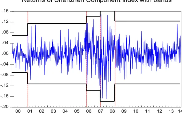
4.3 Identification of Sudden Breaks in Volatility ...54
4.4 Estimation of Conditional Volatility Models ...57
4.5 In-sample Forecast of GARCH(1,1) Model ...61
5. Summary ...66
6. Conclusions ...70
Bibliography ...72
List of Abbreviations ...76
Declaration of Utilization of Results from this Diploma Thesis List of Annexes
6
1. Introduction
Recently years, financial model of time series take a significant role in plenty of financial industrial, even in decision making and economic forecast. One of the popular models is created for volatility, which has been developed by an extensive literature. At the same time, volatility model is widely applied in analyzing the characteristics of financial market, and testing some specific financial situations.
Especially in liquid stock market, volatility is considered a symptom. Generally increase stock market volatility brings a large stock price change of advances or declines. And then the raise of volatility is usually interpreted as an increase of risk in stock investment, which force investors shift their capital to less risky assts. Thus analysis of volatility in stock market makes some important sense, as our purpose of writing this diploma thesis. Absolutely, not only in stock market, volatility modeling is important for many issues, including leverage ratios, credit spreads, derivative pricing and portfolio decisions.
The traditional econometrics assumes that the volatility or variance of time series variables is constant, which is not practical. As an example, people recognized that the volatility of stock price return is not stable as time changing. It means that traditional econometrics cannot explain the fact well. In addition, according to the perspective of econometric inference, the loss in asymptotic efficiency from neglected heteroskedasticity may be extreme large. Therefore some of conditional heteroskedastic variance models are created for volatility measuring, such as ARCH GARCH, FIGARCH, IGARCH, EGARCH and so on.
In times of low market volatility, it is relatively easy to understand volatility dynamics and modeling volatility. But in some of times, volatility of financial time series is affected by infrequent market structural breaks, corresponding to economic turmoil. Examples include the 1997 Asian currency crisis, the IT dot com bubbles, and the recent global crisis in 2007 ~ 2010. During such periods, apparent spikes in volatility and large movements in asset prices complicate estimation and forecasting of volatility and understanding tis dynamics. These crises or political events dramatically influenced market volatility and diversification
7
opportunities for investors.
The most conditional heteroskedastic variance models do not consider the shift or sudden break in volatility. However, there may be lots of potentially shock in volatility in fact, especially in emerging market. Thus, it is important to take account of these break events, when we estimate volatility persistence.
The main goal of this thesis is to identify sudden breaks in volatility and determine an impact of these breaks on the volatility of stock market. For the propose of this thesis, we use weekly time series of Chinese and U.S. stock markets, covering the period of 2000 ~2014 years. And then, the primary aim will be fulfilled by 3 steps.
In first stage, in order to detecting sudden breaks in both stock markets, we will utilize data samples with a help of the Iterated Cumulative Sums of Squares or ICSS algorithm. In this thesis, Chinese stock market is represented by Shenzhen Component Index, while American stock market is approximated by Dow Jones Industrial Average or DJIA Index.
Next step, we will evaluate an impact of sudden breaks on volatility persistence or long memory, by using General Autoregressive Conditional Heteroskedasticity (GARCH) mdoel and Fractional Integrated General Autoregressive Conditional Heteroskedasticity (FIGARCH) models.
Finally, there will be an in-sample test for fitting degree. And the forecasting ability would be presented as the performance of comparison between actual variances and expected variances, which is created by above-mentioned conditional heteroskedastic variance models.
This paper is divided into 6 chapters, and organised as follows:
The first chapter was the introduction of this thesis, and the main goal was presented as previous mentions.
Chapter 2 will describe some features and application of high frequency financial data. Firstly, there will introduce some characteristics of financial time series, including leptokurtic distribution, volatility clustering and leverage effect of volatility, which features will be observed in empirical application. And then, some important assumptions of financial time
8
series are necessary to be mentioned and considered in our thesis, in order to construct conditional variance model. Finally, the microstructure of financial market will be presented.
Chapter 3 is about the methodologies of volatility model with and without shifts. Initially, we should know what kinds of conditional variance model will be used in this thesis. Afterwards, this chapter will provide the modeling estimation procedures and the criteria of model selection. Last stage, not only Iterative cumulative sum of squares or ICSS algorithm, which is the most significant method, but also models with dummy variables will be introduced.
Chapter 4 will provide the empirical application for achieving our goals. In this chapter, mentioned methods in Chapter 3 and important description of frequency financial data in Chapter 2 will be used. First and foremost, the investigated stock markets will be described. And then some analysis of statistical features will be presented about selected stock index. Furthermore, the main goal, identification of shock breaks and analysis of volatility persistence, will be discussed. In the final step, in-sample analysis will be present for testing the quality of GARCH(1,1) model with and without dummy variables.
Chapter 5 is the summaries for results of Chapter 4. All of the results of Chapter 4 will be listed and described specifically.
In the last chapter, there will be the conclusions of this thesis.
Ultimately, it must be claimed that all original data are received from public sources, and all of tables and figures are made by own calculations in EViews and R software.
9
2. High Frequency Data in Finance
High frequency data in finance are observations on financial variables taken daily or at a finer time scale. In addition, there is often irregularly interval over time. The excellent applications of high-frequency financial data sets in financial econometrics are provided by Andersen (2000), Campbell, Lo and MacKinlay (1997), Dacarogna et. al. (2001), Ghysels (2000), Goodhart and O‘Hara (1997), Gouri´eroux and Jasiak (2001), Lyons (2001), Tsay (2001), and Wood (2000).
These high-frequency financial data sets have been widely used to study various market microstructure related issues, including price discovery, competition among related markets, strategic behavior of market participants, and modeling of real time market dynamics. Moreover, high-frequency data are also useful for studying the statistical properties, volatility in particular, of asset returns at lower frequencies by Ruey S (2005).
In this chapter, we will introduce some features and application of high frequency financial data.
2.1 Characteristic Features of Financial Time Series
In this subchapter, we will provide some characteristic features of financial time series, which include definition and some important parts like Leptokurtic distribution, volatility clustering and leverage effect, as defined by Jürgen and Christian M (2011).
In the first place, there are some descriptions of time series. A time series is that ordering and forming each numerical statistical indicator of a phenomenon according to time sequence, typically consisting of successive measurements made over a time interval. Time series method is a quantitative prediction method, also called simple extension method. Besides time series method is widely used as a common forecast method in statistics.
10
Furthermore, time series analysis is a kind of dynamic data processing method of statistics. The method is based on random process theory and mathematical statistical methods. At the most important point, time series analysis try to find some statistics law for selection random data sequence, then used for solving practical problems. If we use a model to predict future values based on previously observed values, this method can be call time series forecasting by Bauwens (2012).
When it comes to financial time series analysis, there are 2 key features for distinguishing financial time series analysis from other time series analysis.
Financial time series analysis is more concerned with the theory and practice of asset valuation than others.
Financial time series analysis is a highly empirical discipline, but like other scientific fields theory structures the foundation for making inference.
Last but not least, both financial theory and its empirical time series contain a few of uncertainty. For example, there are various definitions of asset volatility, and for a stock return series, the volatility is not directly observable. Due to a result of the added uncertainty, statistical theory and methods play an important role in financial time series analysis.
2.1.1 Leptokurtic Distribution
First and foremost, we must provide some descriptions of central moment measurement for understanding leptokurtic distribution. It is necessary to think about leptokurtic distribution, because most financial time series are not normal distribution and present a fat tails and excess kurtosis. And then let us look at this example:
The ξ th moment of a continuous random variable X is defined as:
𝐸(𝑋𝜉) = ∫+∞𝑥𝜉𝑓(𝑥)𝑑𝑥
11
Where E stands for expectation and f(x) is the probability density function of X. There are 4 measurements of central moment:
The first central moment: mean (𝑥̅) or expectation of X. It measures the central location of the distribution.
The second central moment: variance of X (𝜎𝑥2) or standard deviation of X (𝜎𝑥). This
central moment measures the variability of X.
The first two moments of a random variable uniquely determine a normal distribution. For determination of other distributions, we should consider third and fourth central moment.
The third central moment: skewness. Commonly we use skewness to measure the symmetry of X with respect to its mean, as followed:
𝑆𝑘𝑒𝑤𝑛𝑒𝑠𝑠 (𝑥) = 𝐸 0(𝑋−𝜇𝑥)3
𝜎𝑥3 1 . (2.2)
The fourth central moment: kurtosis. It used to measures the tail behavior of X usually, as followed:
𝐾𝑢𝑟𝑡𝑜𝑠𝑖𝑠 (𝑥) = 𝐸 0(𝑋−𝜇𝑥)4
𝜎𝑥4 1 . (2.3) The amount of K(x) − 3 is called the excess kurtosis because kurtosis of normal distribution is 3. Thus, the excess kurtosis of a normal random variable is zero. According to the value of K(x), we can find 2 types distribution with different unusual kurtosis shape:
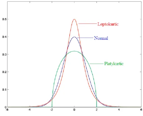
a) Leptokurtic distribution: A distribution with positive excess kurtosis would have heavy tails, implying that there are more mass of its support on the distribution tails than a normal distribution tails. In practice, this means that a random sample from such a distribution tends to contain more extreme values and mean value. For equity investment, leptokurtic distribution means most investors get profit in bull market and most investors experience loss in bear market. Besides fat tails imply volatility with long time-horizon.
12
b) Platykurtic distribution: A distribution with negative excess kurtosis has short tails (e.g., a uniform distribution over a finite interval). It means that there are less mass of its elements on the tails than a normal distribution.
The amount of K(x) − 3 is called the excess kurtosis because kurtosis of normal distribution is 3. Thus, the excess kurtosis of a normal random variable is zero. According to the value of K(x), we can find 2 types distribution with different unusual kurtosis shape:
There is a clearly presentation about the difference between leptokurtic, normal and platykurtic distribution in Figure 2.1.
Figure 2.1: Distribution comparison among leptokurtic, normal and platykurtic
13
2.1.2 Volatility Clustering
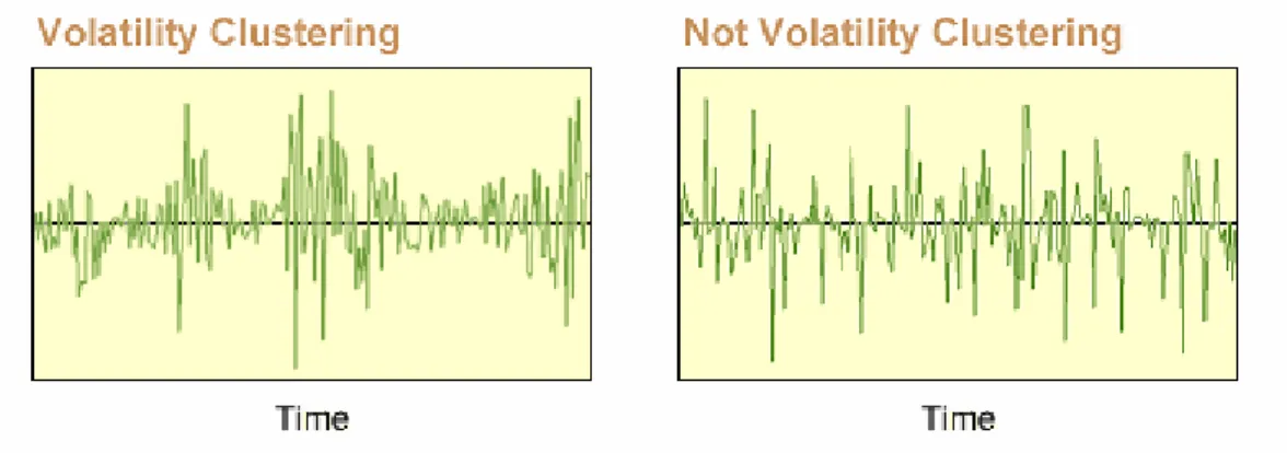
Market prices tend to exhibit periods of high and low volatility. This sort of behavior is called volatility clustering. In finance area, volatility clustering is observed by Mandelbrot(1963), which say "large changes tend to be followed by large changes, of either sign, and small changes tend to be followed by small changes."
There is an example that situation of volatility clustering and non-clustering, which is presented in Figure 2.2, as followed:
Figure 2.2: Phenomenon of volatility clustering and non-clustering
Source form: http://www.riskglossary.com/link/volatility_clustering.htm
Moreover, there is a quantitative manifestation of this fact: while returns are uncorrelated each other, absolute returns |𝑟𝑡| or their squares display a positive, significant and slowly
decaying autocorrelation function corr(|𝑟𝑡|, |𝑟𝑡+ 𝜏|) > 0 for τ ranging from a few minutes
to several weeks, by Tsay, Ruey S (2005). It means that the slow decay behavior in autocorrelation functions of absolute returns is actually directly related to the degree of clustering of large fluctuations within the financial time series.
Since phenomenon of volatility clustering has intrigued many researchers and development in finance such as financial forecasting and derivatives pricing, GARCH models and stochastic volatility models are used primarily to model this phenomenon. In addition, the ARCH by Engle (1982) and GARCH by Bollerslev (1986) models aim to more accurately describe the phenomenon of volatility clustering and related effects such as kurtosis.
14
2.1.3 Leverage Effect of Volatility
One main theory that considers the relationship between volatility and equity price is the leverage effect by Black (1976) and Christie (1982). With the leverage effect, a negative return (declining price) increases financial leverage, making the stock riskier and increasing its volatility. The presence of the leverage effect would imply that the negative innovation (news) has a greater influence on volatility than a positive innovation (news).
Since the leverage effect is a phrase that describes the asymmetric response of volatility to shocks of differing signs, ‗‗leverage effects‘‘ have become synonymous with asymmetric volatility. Black (1976) and Christie (1982) were among the first to document and explain a negative relationship between current individual stock return and future volatility in the US equity markets.
Black (1976) showed that if the price on day t fell then the volatility on day t + 1 would, on average, be higher than if the price rose by the same amount. Black's explanation of this phenomenon stated that a price fall would reduce the value of equity and hence increases the debt-to-equity ratio. Because this increase in leverage that raises the riskiness of the firm, we can observe an increase in volatility.
Christie (1982) tested Black's explanation by looking at the relationship between the asymmetry in equity volatility and the debt-to-equity ratio of firms. At the beginning he demonstrates that stock price changes and volatility are inversely related. For example, the elasticity of volatility with respect to the value of equity is negative. In addition, he also finds that volatility is an increasing function of financial leverage suggesting that this may be the cause of the negative elasticity of volatility with respect to the value of equity. He found a strong relationship between the leverage effect and the debt-to-equity ratio, but claimed that the debt-to-equity ratio cannot fully explain the effect. If such asymmetries volatility exist in individual stocks returns, it is natural to expect that in a cross sectional analysis the size of the asymmetry will be positively related to the degree of financial leverage. For example, the higher the leverage will lead to the more asymmetric the response of volatility to innovations.
15
Otherwise the asymmetric impact of innovations on volatility has to be explained by factors other than the financial leverage.
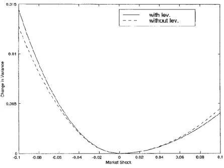
Figure 2.3: Asymmetric volatility
Source form: GeertBekaert(2000) and GuojunWu (2000)
This Figure 2.3 shows the market shock impact on market variance with or without incorporating the change in leverage level. The shocks are at the firm, not equity, level. Leverage ratios are evaluated at the sample mean except when leverage effects are taken into account.
2.2 Assumptions of Financial Time Series
According to our mention in 2.1, we know that the financial time series is a set of financial observations for a variable over successive periods of time. Here we simply discuss the most application in financial time series analysis. That is linear regression analysis, also called ordinary least squares (OLS) regression analysis.
16
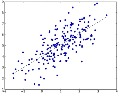
In statistics, ordinary least squares (OLS) or linear least squares is a method for estimating the unknown parameters in a linear regression model, with the goal of minimizing the differences between the observations in some arbitrary dataset and the responses of prediction by the linear approximation of the data (visually this is seen as the sum of the vertical distances between each data point in the set and the corresponding point on the regression line - the smaller the differences, the better the model fits the data).
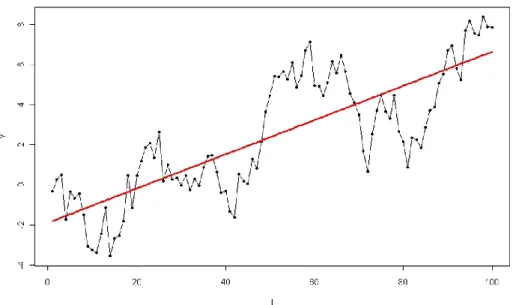
There is a Figure 2.4, which presents an example of linear regression model by using ordinary least squares, as followed:
Figure 2.4: Linear regression model by ordinary least squares
Source from: http://mlpy.sourceforge.net/docs/3.3/lin_regr.html
For analyzing financial time series correctly, we must apply some assumption of linear regression. To ensure unbiased estimation and correct p-value, the main assumptions include:
A linear relationship exists between the dependent and the independent variable.
The independent variable is uncorrelated with the residuals and each other.
The expected value of the residual term is zero. It means make a zero conditional mean assumption.
17
The variance of the residual term is constant for all observations. It is known as homoscedasticity.
The residual term is independently distributed; that is, the residual for one observation is not correlated with that of another observation. It is a statistical description as no autocorrelation.
The residual term is normally distributed.
Then we divided previous 6 assumptions into 3 classifications, included normality, linearity and stationarity.
2.2.1 Linearity
That a linear relationship exists between the dependent and the independent variable is the assumption of linearity. In common application, linearity is referred to a mathematical relationship or function that can be graphically represented as a straight line, as in two quantities that are directly proportional to each other, such as the mass and weight of an object.
In financial time series, we need assume there is linearity between the object values (dependence) and time series (independence). This relationship can be presented as followed formula and Figure 2.5:
𝑦𝑡 = + 𝑡 + 𝑡 , (2.4)
: Coefficient of constant (intercept at the vertical axis),
: Slope coefficient,
18
Figure 2.5: Linearity time series model
Source from: Rabett (2010)
Comparing with linearity time series model, we can present a non-linearity time series model as followed formula:
𝑦𝑡 = 𝑒 + 𝑡+
𝑡 . (2.5)
and the Figure 2.6:
Figure 2.6: Non-linearity time series model
19
2.2.2 Normality
The next assumption can be called normality, which is important assumption for the autocorrelation test. In addition, normality is the precondition for construction of point forecasts and interpretation of the estimated parameters.
It means the residual term must follow normal distribution. The residual can be presented as:
𝑡 = 𝑦𝑡 𝑦̂𝑡 , (2.5)
𝑦𝑡: The value of the time series or the dependent variable at time t,
𝑦̂𝑡: The predicated value of y, which is the dependent variable at time t.
In probability theory, the normal or Gaussian distribution is a very commonly occurring continuous probability distribution—a function that tells the probability that any real observation will fall between any two real limits or real numbers, as the curve approaches zero on either side. Normal distributions are extremely important in statistics and are often used in the natural and social sciences for real-valued random variables whose distributions are not known.
We can simply compare the difference between normal distribution and non-normal distribution by the Figure 2.7.
20
Figure 2.7: Comparing between normal distribution and non-normal distribution
Source from: Hun Myoung Park (2009)
Besides, we must discuss the application of Jarque-Bera statistic, which is often used to test the null of whether the standardized residuals are normal distribution. Jarque-Bera test give us the result of probability of normally distributed instead of leptokurtic distribution, by testing skewness and kurtosis simultaneously.
The assumption of Jarque-Bera is that the third moment of skewness in normal distribution is zero and forth moment of kurtosis in normal distribution is 3. So the JB statistic is be defied as:
= (𝑆𝐾2+ 𝐾𝑈2) , (2.6)
where the SK is the test reiteria of skewness, it can be expressed as:
𝑆𝐾 = ( ) (̂3
̂3) , (2.7)
and the KU of kurtosis test criteria is descripted as follows:
𝐾𝑈 = (2 ) (̂4
̂ ) , (2.8)
while
21
Under the assumption of normality of unsystematic component, both statistics SK and KU have normal distribution N(0,1). However JB statistic has the distribution of 2( ). In fact, not only non-normality of unsystematic component but also the heteroskedastic unsystematic component can result in refusing the null hypothesis.
2.2.3 Stationarity
The rest 4 assumptions are about stationarity assumption.
In mathematics and statistics, a stationary process is a stochastic process whose joint probability distribution does not change as the shift of time. Ultimately, if parameters such as the mean and variance are presented, would also do not change over time and do not follow any trends.
Stationarity is used as a tool for time series analysis, where the raw data is often transformed to become stationary; for example, economic data are often seasonal and/or dependent on a non-stationary price level.
According to previous description, we can see some difference between stationarity and non-stationarity in Figure 2.7 as follows:
22
Figure 2.7: Comparing between stationarity and non-stationarity
Source from: Nils Bohr, Thomson and Box
The foundation of time series analysis is stationarity. A time series *𝑟𝑡+ is said to be strictly stationary if the joint distribution of (𝑟𝑡 , , 𝑟𝑡 ) is identical to that of
(𝑟𝑡 +𝑡, , 𝑟𝑡 +𝑡) for all t, where k is an arbitrary positive integer and (𝑡 , , 𝑡 ) is a
collection of k positive integers. In other words, strict stationarity requires that the joint distribution of (𝑟𝑡 , , 𝑟𝑡 ) is invariant under time shift. This is a very strong condition that
is hard to verify empirically.
A weaker version of stationarity is often assumed. A time series *𝑟𝑡+ is weakly stationary
if both the mean of 𝑟𝑡 and the covariance between 𝑟𝑡 and 𝑟𝑡− are time-invariant, where
is an arbitrary integer. More specifically, *𝑟𝑡+ is weakly stationary if:
a) (𝑟𝑡) = , which is a constant, and
23 T data points *𝑟𝑡|𝑡 = , , 𝑇+.
The weak stationarity implies that the time plot of the data would show that the T values fluctuate with constant variation around a fixed level. In applications, weak stationarity enables one to make inferences concerning future observations (e.g., prediction).
The covariance = o (𝑟𝑡, 𝑟𝑡− ) is called the lag- autocovariance of 𝑟𝑡. It has two
important properties: (a) = r(𝑟𝑡) and (b) = . The second property holds
because o (𝑟𝑡, 𝑟𝑡−(− )) = o (𝑟𝑡−(− ), 𝑟𝑡) = o (𝑟𝑡+ , 𝑟𝑡) = o (𝑟𝑡 , 𝑟𝑡 − ) , where
𝑡 = 𝑡 + .
In the finance literature, it is usual to assume that an asset return series is weakly stationary. This assumption can be checked empirically provided that an enough number of historical returns are available.
2.3 Microstructure of Financial Markets
It is important to know microstructure of financial markets, when us try to price financial assets value and understand their internal design concept. There is a common definition of market microstructure, ―It is the study of the trading mechanisms used for financial securities‖, which is defined by Maureen O‘Hara (1995) of Cornell University. She is an authority on market microstructure, describes market microstructure as ―the study of the process and outcomes of exchanging assets under a specific set of rules.‖
In addition, National Bureau of Economic Research (NBER) defines market microstructure as a field of study, which is devoted to theoretical, empirical, and experimental research on the economics of security markets. This study includes the role of information in the price discovery process, the definition, measurement and control of liquidity, and transaction costs and their implication for efficiency, welfare, and regulation of alternate trading mechanisms and market structures.
24
superficial level. But market microstructure is much more than that. Market microstructure has broader interest among financial economists, since it has implications for asset pricing, international finance and corporate finance. A basic assumption of market microstructure theory is that asset prices need not reflect information expectations value fully due to a variety of frictions. Thus, market microstructure is related to the field of investments, which is care about the equilibrium value of financial assets. Market microstructure is also linked to traditional corporate finance, since difference between price and value has the potential to affect financing and capital structure decisions. The relationship between market microstructure and other areas of finance is relatively new and is continuing to evolve.
Furthermore market microstructure is a branch of finance concerned with the details of how exchange happens in financial markets. While the theory of market microstructure applies to the exchange of real or financial assets, more evidence is available on the microstructure of financial markets due to the availability of transactions data from them. The major thrust of market microstructure research examines the ways in which the working processes of a market affects determinants of transaction costs, prices, quotes, volume, and trading behavior. Recently innovations have allowed an expansion into the study of the impact of market microstructure on the incidence of market abuse, such as insider trading, market manipulation and broker-client conflict.
The most application of market microstructure can be summarize into 4 parts:
Market structure and design issues: it focuses on the relationship between price determination and trading rules.
Price formation and discovery: it concentrates on the process by which the price for an asset is determined.
Transaction cost and timing cost: it pays attention to transaction cost and timing cost and the impact of transaction cost on investment returns and execution methods.
Information and disclosure: it cares about the market information and transparency and the impact of the information on the behavior of the market participants.
25
3. Volatility Modeling
In recent years, volatility modeling became a popular studying in analyze the characteristics of financial market. And then an extensive literature has been developed for volatility analysis.
There is a traditional econometrics assumption that the volatility or variance of time series variables is constant, which is not practical. As an example, people recognized that the volatility of stock price return is not stable as time changing. It means that traditional econometrics cannot explain the fact well.
Understanding the accurate relationship between volatility and time, is crucial for many issues in macroeconomics and finance, such as irreversible investments, option pricing, the term structure of interest rates, and general dynamic asset pricing relationships. In addition, according to the perspective of econometric inference, the loss in asymptotic efficiency from neglected heteroskedasticity may be extreme large.
When evaluating economic forecasts, a much more accurate estimate of the forecast error uncertainty is generally available by conditioning on the current information set. It is the basic methodology of variance analysis.
In this chapter, we will describe some of volatility analysis models, which will be applied in empirical analysis of financial time series. There will be some of models, which can capture both long memory and nonlinear dynamics jointly in volatility process. They include ARCH model, GARCH model, FIGARCH model and the ICSS algorithm.
3.1 ARCH Model
For giving up this shortcoming and getting more accurate estimate of error, Autoregressive conditional heteroskedasticity model or ARCH model is presented by Robert F. Engle (1982). Engle obtained the 2003‘s Nobel Prize of economy by ARCH model.
26
ARCH models are used to descript and model observations. They are used whenever there is reason to believe that, the error terms will have a characteristic size or variance at any point in a series. In particular ARCH models assume the variance of the current error term to be a function of the actual sizes of the previous time periods' error terms. Furthermore, the variance is often related to the squares of the previous error term.
ARCH models are used commonly in modeling financial time series for exhibiting time-varying volatility clustering. ARCH-type models are sometimes considered to be part of the family of stochastic volatility models, but strictly this is incorrect. Because we can get a completely pre-determined volatility at time t by given previous values.
For construction of ARCH model, firstly we need understand the equation of linear regression model, which is the workhorse of economic modeling. A univariate linear regression represents a proportionality relationship between two variables:
𝑦𝑖 = 𝛼 + 𝑥 + 𝑖 . (3.1)
The preceding linear regression model presents that the expectation of the variable y is times the expectation of the variable x plus a constant 𝛼. The proportionality relationship between y and x is not exact but subject to an error . In standard regression theory, the error is assumed to have a zero mean and a constant standard deviation 𝜎. The standard deviation is the square root of the variance, which is the expectation of the squared error:
𝜎2 = 𝐸( 2) . (3.2)
It is a positive number that measures the size of the error. We call the assumption is homoscedasticity, when the expected size of the error is constant and does not depend on the size of the variable x. If the expected size of the error term is not constant, we call it as heteroskedasticity.
In describing ARCH/GARCH behavior, we focus on the error process. In particular, we assume that the errors are an innovation process, that is, we assume that the conditional mean of the errors is zero. We write the error process as:
27
where 𝜎𝑡is the conditional standard deviation and the 𝑧 terms are a sequence of independent,
zero-mean, unit-variance, normally distributed variables. Under this assumption, the unconditional variance of the error process is the unconditional mean of the conditional variance. However the unconditional variance of the process variable does not coincide with the unconditional variance of the error terms in general.
Secondly, when we discuss financial and economic models, conditioning is often stated as regressions of the future values of the variables on the present and past values of the same variable. For example, if we assume that time is discrete, we can express conditioning as an autoregressive model:
𝑥𝑡+ = 𝛼 + 𝑥𝑡+ ⋯ ⋯ + 𝑛𝑥𝑡−𝑛+ 𝑡+ . (3.4)
The error term 𝑖 is conditional on the information 𝐼𝑖 that, in this example, is represented by the present and the past n values of the variable 𝑥.
Besides the simplest autoregressive model is:
𝑥𝑡+ = 𝛼 + 𝑥𝑡+ 𝑡+ . (3.5)
Thirdly, we can construct the simplest autoregressive conditional heteroskedasiticity model as Robert F. Engle invented in 1982:
𝑡2 = 𝛼 + 𝛼 𝑡− 2 + 𝑢𝑡 , (3.6)
where 𝑡is the error term of 𝑥𝑡 In addition, 𝑢𝑡 is the error term of 𝑡. Furthermore this formula is called ARCH(1) model, since in t time is correlated with in only t-1 time or one lagged value. Under an ARCH model, if the residual return is large in magnitude, there is a high probability that next period‘s conditional volatility 𝜎𝑡2 will be large in our forecast.
According to formula 3.2, we can improve the formula 3.6 in:
𝜎𝑡2 = 𝑣𝑎𝑟(
𝑡| 𝑡− ) = 𝐸( 𝑡2) = 𝛼 + 𝛼 𝑡− 2 . (3.7)
In formula 3.7, there is no implication that ARCH(1) is non-stationary. It is just stating, that 𝜎𝑡2 and
t− 2 are correlated. Due to 𝜎𝑡2 ≥ 0, 𝛼 ≥ 0 and 𝛼 ≥ 0 must to be ensured
28
1. If 𝛼 = 0, the conditional variance must equal with 𝛼 . And then this time series is covariance stationary.
2. If 𝛼 = 0, the conditional variance will change with fluctuation of t− 2 . So this time series can not be said that meet the requirement of covariance stationary.
Moreover, when 𝛼 meets the condition of 0 < 𝛼 < , we can get the mean-reverting level according to mean reversion of ARCH(1) model by formula:
𝜎2 = 2 = 𝛼
− 𝛼 . (3.8)
According to this formula 3.8, we know the more 𝛼 close to 1, the more probability that this time series model is not covariance stationary or heteroskedasticity. On contrary, there is high probability to say it is covariance stationary or homoscedastic by Husek (2007).
Last but not least, since the ARCH(1) states that the conditional variance depends only on 1 lagged value, ARCH(1) is a simplest autoregressive conditional heteroskedasticity model and not practical. In fact, we should consider more lagged value, which have significant influence. Generally we consider that the ARCH(1) model is the ARCH(q) model‘ 1 order. So we can extend ARCH model to q order and express it as:
𝑡2 = 𝛼 + 𝛼 𝑡− 2 + 𝛼2 𝑡−22 + ⋯ ⋯ + 𝛼𝑞 𝑡−𝑞2 + 𝑢𝑡 . (3.9)
Same as formula 3.7, we can get the expectation formula as:
𝜎𝑡2 = 𝑣𝑎𝑟( 𝑡) = 𝐸( 𝑡2) = 𝛼 + 𝛼 𝑡− 2 + 𝛼2 𝑡−22 + ⋯ ⋯ + 𝛼𝑞 𝑡−𝑞2 . (3.10)
As the result of formula 3.10, the conditional variance 𝜎𝑡2 depends on q lagged values.
Only the effect of a shock happen between time q and time t that will be expressed by their coefficient 𝛼. But there will be no a influence for 𝜎𝑡2, if the periods older than q.
And then we can construct the mean-reverting level for ARCH(q):
𝜎2 = 2 = 𝛼
− ∑𝑞𝑖= 𝛼𝑖 . (3.11) Same as the analysis of covariance stationary in ARCH(1), we can get the same conclusion.
29
If 𝛼𝑖 = 0, we can conclude that the ARCH(q) model fulfill the conditions of covariance
stationary. So the long term conditional variances 𝜎𝑡−𝑖2 are consistent and equal to
unconditional variance 𝜎2.
There are some shortcomings about the application of ARCH model in volatility analysis:
1. The first problem is the strict condition of non-negativity for all coefficients in the conditional variance equation.
2. And then the most important problem is the parameters estimation and significant test. As the amount of q orders increase, the restrict condition will be much more complicated. In most actual regression analysis, these conditions can not be fulfilled easily.
3. Last, there is also a problem to determine the length of delay squares residuals q. It means we should know how many order will be used in ARCH(q) model.
3.2 GARCH Model
In order to improve these shortcomings of ARCH(q), autoregressive conditional heteroskedasticity model were generalized by many ways. And the most popular way is generalized ARCH, or GARCH model by Bollerslev (1986) and Taylor (1986). The GARCH process is often preferred by financial modeling professionals. It provides a more practical context than other forms, when trying to predict the prices and rates of financial instruments.
This model is also a weighted average of past squared residuals, but it has declining weights that never go completely to zero. In its most general form, it is not a Markovian model, as all past errors contribute to forecast volatility. It gives parsimonious models that are easy to estimate and, even in its simplest form, has proven surprisingly successful in predicting conditional variances especially in case of small selections. The GARCH model specified the conditional variance to be a function of lagged squared errors and past conditional variance, which replace the infinite length of delay q and expectation parameters in ARCH(q) model.
30
The most widely used GARCH specification asserts that the best predictor of the variance in the next period is a weighted average of the long-run average variance, the variance predicted for this period, and the new information in this period that is captured by the most recent squared residual. Such an updating rule is a simple description of adaptive or learning behavior and can be thought of as Bayesian updating.
Firstly we should understand the simplest GARCH model, which can be presented as:
𝑡2 = 𝛼 + 𝛼 𝑡− 2 + 𝜎𝑡− 2 + 𝑢𝑡 , (3.12)
where the 𝑢𝑡 is the white noise followed random distribution in time t and defined as
𝑡2 𝜎𝑡2. In addition, the 𝜎𝑡− 2 is the past conditional variance, which is most use the
weighted average of the long-run average variance.
And then if we improve the formula 3.12 as we do in ARCH model, we can get:
𝜎𝑡2 = 𝑣𝑎𝑟( 𝑡| 𝑡− ) = 𝐸( t2) = 𝛼 + 𝛼 𝑡− 2 + 𝜎𝑡− 2 . (3.13)
GARCH model described in formula 3.13 and typically referred to as the GARCH(1,1) model, which is widely used. This name derives from the fact that the 1,1 in parentheses is a standard notation, in which the first number refers to the number of autoregressive lags or ARCH terms and the second number refers to the number of moving average lags specified or often called the number of GARCH terms.
GARCH(1,1) model is better to explain volatility clusters than ARCH model. And then there is a same requirement for ensure non-negativity conditional variance 𝜎𝑡2, which means
all these three parameters must be non-negativity, like 𝛼 ≥ 0, 𝛼 ≥ 0 and ≥ 0.
Furthermore similarly to ARCH model, if 𝛼 and are between 0 and 1, we can also get the mean-reverting level by:
𝜎2 = 2 = 𝛼
− (𝛼 + ) . (3.14)
When this GARCH(1,1) model is covariance stationary, the value of 𝛼 + must be close to 0. Absolutely if the value of 𝛼 + is close to 1, GARCH(1,1) is not covariance stationary. In addition, when we analyze the long memories effect of market shock, we can
31
conclude that the more close to 1, the more persistence influence of shock will be.
Secondly if we expend GARCH(1,1) model to GARCH(p,q) model, it can be processed as:
𝜎𝑡2 = 𝛼 + ∑ 𝛼 𝑖 𝑡−𝑖2 𝑝
𝑖= + ∑𝑞 = 𝜎𝑡− 2 , (3.15)
where the p is the length of delay 𝑡2and q represents the maximal length of delay 𝜎 𝑡2.
Besides the conditional variance should meet the requirement of non-negativity, which means
𝛼 ≥ 0, 𝛼𝑖 ≥ 0 and ≥ 0.
Same as the GARCH(1,1), when (𝛼 + ) (𝛼2+ 2) ⋯ (𝛼 + ) ≤ is fulfilled, there is also a mean-reverting level in GARCH(p,q):
𝜎2 = 𝛼
−, (𝛼 + )−(𝛼 + )−⋯⋯−(𝛼𝑚+ 𝑚)- . (3.16) Even though the GARCH(p,q) is widely useful and popular way in construction of model, there are still some limitations for application by Husek (2007):
1. In practical application, some of the estimated parameters can not meet the requirement of non-negativity.
2. The GARCH models are not able to explain the leverage effect, which means the asymmetric volatility mentioned in chapter 2.
3. It is hard to get the feedback between conditional variance and conditional average of regression model directly.
3.3 FIGARCH Model
In this subchapter, we consider another modification of ARCH family models to avoid some shortcoming of ARCH model. This model is Fractional Integrated GARCH morel or FIGARCH model by Baillie, Bollerslev, and Mikkelsen (1996).
32
The importance of introducing FIGARCH model was, this model provided a greater flexibility process for modeling the conditional variance. In addition, FIGARCH model is able to explain and represent the observed temporal dependencies in financial market volatility. Particularly the FIGARCH model allows only a slow hyperbolic rate of decay for the lagged squared or absolute innovations in the conditional variance function. What is more, this model can accommodate the time dependence of the variance and a leptokurtic unconditional distribution for the returns with some structure shifts on long memory of volatility.
By Baillie, Bollerslev, and Mikkelsen (1996) description, we can improve the GARCH(1,1) model and define the FIGARCH(1,d,1) model for a conditional variance as:
𝜎𝑡2 = 𝛼 ( )− + , ( 𝐿)− ( 𝛼 𝐿)− ( 𝐿)𝑑- 𝑡2 , (3.17)
where d is the fractional difference parameter, which fulfill the condition of 0 ≤ 𝑑 ≤ . Besides L means the lag operator, and ( 𝐿)𝑑 present the first difference operator with the
fractional difference parameter d.
When we use FIGARCH model to estimate volatility of persistence shocks, either the conditional variance or the level of long memory will be measured by the fractional differencing parameter d, which is estimated by quasi-maximum likelihood estimation technique.
3.4 Modeling Estimation Procedures
As we mentioned in previous sub-chapter, we should also develop an idea to establish the procedures of volatility models. Generally, the procedures can be divided into the following steps:
1. Determine a suitable linear or nonlinear model, based on the specified time series.
2. Test the hypothesis of conditional homoskedasticity against the alternative hypothesis of conditional heteroskedasticity for linear and nonlinear type.
33
3. Estimate the parameters of selected model for conditional heteroskedasticity.
4. Make a verification of suitability in the given model.
5. Make some modification for the model, if necessary.
6. Use the model for descriptive or predictive purposes.
3.5 Criteria for the Model Selection
There can be more than one acceptable estimated model, when analyzing the same time series. There are some methods available to choose the optimal one. The idea for choosing the optimal estimated model is to compare the residuals of each estimated model by the summary statistics.
Firstly, the best suitable estimation model can be chosen by the order of differentiation. The criteria are Akaike or AIC and Schwartz-Bayes or SBC by Arlt (2003).
Akaike information criterion can be expressed as:
𝐴𝐼𝐶(𝑀) = 𝑇 𝑙𝑛 𝜎̂𝜀2+ 𝑀 , (3.18)
where the 𝑀 = 𝑝 + 𝑞 is the number of parameters in ARMA(p,q) model and 𝜎̂𝜀2 is the
residual variance of this model. The result of minimum value of this criterion should be chosen.
And then, the Schwartz-Bayes criteria can be described as followed:
𝑆 𝐶(𝑀) = 𝑇 𝑙𝑛 𝜎̂𝜀2+ 𝑀 𝑙𝑛 𝑇 . (3.19)
The difference between formula 3.17 and formula 3.18 is that in equation formula 3.18, T represents the number of observations. This T is equal to the number of residuals obtained from the model. The choose principal of Schwartz-Bayes criteria is same as formula 3.18, which means that the model with the minimum value of statistic will be optimal.
34
Secondly, in order to verify whether the model we have established is accurate enough for prediction, in other ward whether the estimation model can explain the real situation well, we can also use loss functions to make estimation about the size of differences between the theoretical result and actual result.
Root mean square error or RMSE is frequently used for measuring for differences between estimated data and the actual observed data. Basically, the RMSE represents the sample standard deviation of the differences between predicted values and observed values. Formula of RMSE is expressed as:
𝑅𝑀𝑆𝐸 = √∑𝑛𝑡= (𝜎̂𝑡−𝜎𝑡)
𝑛 . (3.20)
Besides, there are also other ways to measure the difference between estimation data and actual data, such as Mean Absolute Errors or MAE, Mean Absolute Percentage Errors or MAPE, Theil‘s Coefficient and so on. These criteria can be defined as follow:
𝑀𝐴𝐸 = ∑𝑡= |𝜎̂𝑡 𝜎𝑡| , (3.21) 𝑀𝐴𝑃𝐸 = ∑ |𝜎̂𝑡−𝜎𝑡| 𝜎𝑡 𝑡= , (3.22) 𝑇h𝑒𝑖𝑙’𝑠 𝑈 = √𝑇 ∑ |𝜎̂𝑡−𝜎𝑡| 𝑇 𝑡= √𝑇 ∑𝑇𝑡= 𝜎𝑡 +√𝑇 ∑𝑇𝑡= 𝜎̂𝑡 . (3.23)
The choice of a loss function is not arbitrary. It is very restrictive and sometimes loss function may be characterized by its desirable properties. In general, the loss function with lower value is the better estimation model, which has higher fitting degree.
Sound economical prediction practice requires selecting an estimator consistent with the actual acceptable variation experienced in the context of a particular applied problem. As a result, in the applied use of loss functions, we should be careful when deciding which statistical method to use to model an applied problem.
35
3.6 Iterative Cumulative Sum of Squares (ICSS) and Modification
In this subchapter, we will discuss the Iterative cumulative sum of squares or ICSS algorithm by Inclán and Tiao (1994) and its modification by Sanso (2004), because this quantitative method is an important algorithm in volatility analysis. Absolutely it will be used in chapter 4 about practical application.
Volatility of stock returns is affected substantially by infrequent sudden changes or regime shifts, corresponding to domestic and global economic events, such as financial crisis.
There will be some systematic effect on the whole market or might only affect a particular sector, when sudden events happen. For achieve efficient portfolios, the most of individual investors prefers to hold mutual funds or sector index funds rather than holding individual securities with some sudden event risk.
Furthermore, the investors and managers of index funds need to determine whether these major events cause shifts in volatility in the whole market or a particular sector, in order to create much better diversified portfolios, predict the future volatility of some index funds properly and get the accurate valuation of them.
However, if we only use the GARCH and FIGARCH approach to analyze the volatility, it is not enough since that GARCH and FIGARCH model are incapable of responding sudden changes. In addition, they are also inappropriate for examinations of volatility persistence.
In order to overcome this problem, the most popular approach is cumulative sums of squares (ICSS) algorithms, which was be stated by Inclán and Tiao (1994). ICSS algorithm is implemented to detect break point in the variance of a stock return series each sub-period.
There is the assumption of ICSS algorithm, which can be divided into 4 paths:
Firstly, financial time series displays a stationary variance over an initial time period.
And then there is a sudden shock that alters the variance when the certain event generates a break point.
36
This process is repeating over the time.
Firstly we should focus on formula 3.4, which is the autoregressive model presented previous subchapter, when we start to explain the ICSS algorithm.
And then Let us assume that * 𝑡+ denote an independent time series with a zero mean and
an unconditional variance, 𝜎2. In addition, the variances of each interval are given by
= 0, , ⋯ , 𝑁 , where 𝑁 is the total number of variance changes in T observations and
< 𝐾 < 𝐾2 < ⋯ < 𝐾𝑁𝑇 < 𝑇 are the set of change points.
To summarize, the unconditional variance 𝜎2 over 𝑁 intervals can be defined as follow:
𝜎𝑡2 = { 𝜎2, < 𝑡 < 𝐾 𝜎2, 𝐾 < 𝑡 < 𝐾 2 ⋮ 𝜎𝑁2𝑇, 𝐾 𝑁𝑇 < 𝑡 < 𝑇 . (3.24)
Secondly a cumulative sum of squares is utilized to for determining the total number of sudden changes in volatility and the time point when each variance break or shift occurs. As the result, the cumulative sum of squares from the first observation to the Kth time point can be expressed as below:
𝐶𝐾 = ∑𝐾𝑡= 𝑡2 , (3.25)
where 𝐾 = 0, , ⋯ , 𝑇.
Thirdly ICSS algorithm is based on DK statistics and tests the null hypothesis of constant unconditional variance. And then DK statistics is computed as follows:
𝐷𝐾 = .𝐶𝐶𝐾
𝑇/
𝐾
, (3.26)
where 𝐷 = 𝐷 = 0. In which 𝐶 is the sum of the squared residuals from the whole sample period. And then we can discuss 2 scenarios by variance stationary analysis as:
a) If there is no changes in variance occur, the 𝐷𝐾 statistic will oscillate around zero. In addition, if 𝐷𝐾 is plotted against K, it will resemble a horizontal line.
37
b) On the other hand, if there are one or more changes in variance occur, then the statistic values are not stable. 𝐷𝐾 will be drift up or down from zero.
In this context, structure changes in variance are detected by the critical values obtained from the distribution of 𝐷𝐾 assuming the null hypothesis of constant variance. Therefore, If
the maximum absolute value of 𝐷𝐾 is greater than the critical value, the null hypothesis of homogeneity can be rejected.
Last, the test proposed by Inclán and Tiao (1994) can be written as follows:
𝐼𝑇 = 𝑠𝑢𝑝𝐾|√𝑇/ 𝐷𝐾| , (3.27)
where √𝑇/ is used to standardise the distribution. And then let us define K* as a value,
which is the point of K when 𝑠𝑢𝑝𝐾|𝐷𝐾| is obtained. If 𝑠𝑢𝑝𝐾|√𝑇/ 𝐷𝐾| exceeds the critical
value, then the parameter K* means the time point when a volatility suddenly changed.
In accordance with the study of Inclán and Tiao (1994), the critical value of 1.358 is the
95th percentile of 𝑠𝑢𝑝𝐾|√𝑇/ 𝐷𝐾| assuming that follow asymptotic distribution. Therefore,
the upper and lower boundaries can be established at ±1.358 in the 𝐷𝐾 plot. So that a
change point in variance is identified, when the value of 𝐷𝐾 exceeds these boundaries.
The ICSS algorithm works by evaluating the 𝐷𝐾 function over different time periods, and those different periods are determined by break points, which are themselves identified by the
𝐷𝐾 plot. This algorithm was widely evidenced that financial data have time-varying variance
and excess kurtosis
However, if the series harbors multiple change points, the 𝐷𝐾 function alone will not be
sufficiently powerful to detect the change points at different intervals. In this regard, Inclán and Tiao (1994) modified an algorithm that employs the 𝐷𝐾 function to search
38
Specifically, recent literature has shown that the ICSS algorithm tends to overstate the number of actual structural breaks in variance. Especially in the behavior of the ICSS algorithm is questionable under the presence of conditional heteroskedasticity, which is point out by Bacmann and Dubois (2002). They show that one way to circumvent this problem is by filtering the return series by a GARCH(1,1) model, and applying the ICSS algorithm to the standardized residuals. Bacmann and Dubois conclude that structural breaks in unconditional variance are less frequent than it was shown previously.
In order to overcome the problem that the size distortions are more extreme for heteroskedastic conditional variance processes, which make ICSS test invalidate in empirical application of financial time series. There are 2 modifications, which are proposed by Sanso et al (2004).
The first statistic k1 is defined as follow:
𝑘 = 𝑠𝑢𝑝𝐾|√ 𝐾| , (3.28) where 𝐾 = 𝐶𝐾−𝐾𝑇𝐶𝑇 √𝜂̂4−𝜎̂4 , (3.29) 𝜂̂ = ∑𝑖= 𝑡 , (3.30) and 𝜎̂2 = 𝐶 . (3.31)
The second statistic k2 is defined as follow:
𝑘2 = 𝑠𝑢𝑝𝐾|
√ 𝐺𝐾| , (3.32)
where assuming that
𝐺𝐾 =
√𝜔̂4.𝐶𝐾
𝐾
39
For estimating 𝜔̂ consistently, there are two possible ways given by Sanso et al (2004). The one ways is a nonparametric estimator, which is defined as:
𝜔̂ = ∑ ( 𝑡2 𝜎̂2)
𝑡= +2∑𝑡= 𝑤(𝑙, 𝑚)∑𝑡=𝑙+ ( 𝑡2 𝜎̂2)( 𝑡−𝑙2 𝜎̂2) . (3.34)
And another ways is parametric estimator, which can be described as:
𝜔̃ = ( ∑𝑝 = 𝜆 )−2𝑇− ∑ 𝑒 𝑡2
𝑡= , (3.35)
where 𝜆 and 𝑒𝑡 are from the regression:
𝑢𝑡 = 𝛿̂ + ∑𝑝 = 𝜆̂ 𝑢𝑡− + 𝑒𝑡 , (3.36)
with 𝑢𝑡 = 𝑡2 𝜎̂2.
Using the modified ICSS algorithm denotes that we are calculating test statistics for various sample sizes. Thus, the critical values for each test statistic might be obtained from a response surface as provided by Sanso et al (2004), as long they provide better results when using small samples.
Last, if we consider that sudden changes in volatility, the principal objectives of this study are twofold with a help of the ICSS algorithm:
1. This study detects the sudden changes using the ICSS algorithm, which is already introduced previously.
2. We examines whether the inclusion of sudden breaks in the GARCH model and FIGARCH model reduces the coefficients of volatility asymmetry and persistence or not.
40
Therefore, conditional variance in the GARCH(1,1) with sudden changes can be defined via the ICSS algorithm as follows:
𝜎𝑡2 = 𝛼 + 𝛼
𝑡− 2 + 𝜎𝑡− 2 + 𝑑 𝐷 + ⋯ + 𝑑𝑛𝐷𝑛 . (3.37)
And then the FIGARCH(1,d,1) models with sudden changes will be described via the ICSS algorithm as:
𝜎𝑡2 = 𝛼 ( )− + , ( 𝐿)− ( 𝛼 𝐿)− ( 𝐿)𝑑- 𝑡2
+𝑑 𝐷 + ⋯ + 𝑑𝑛𝐷𝑛 , (3.38)
where 𝐷 + ⋯ + 𝐷𝑛 denote dummy variables that can be equal the value of 1 when sudden shifts in volatility appears, elsewhere take a value of 0.
41
4. Empirical Applications
The previous Chapter 3 of this thesis was focused on the theoretical methodology. In this chapter, we will combine the mentioned methods and the real financial time series. In addition, the main purpose of this chapter is same as the aim of this thesis. We will examine the impact of structural breaks on volatility persistence of not only developed economies represented by American stock market, but also emerging economics represented by Chinese stock market.
The conducted steps in this chapter will be summarized as follow:
In Subchapter 1, the investigated stock markets will be described.
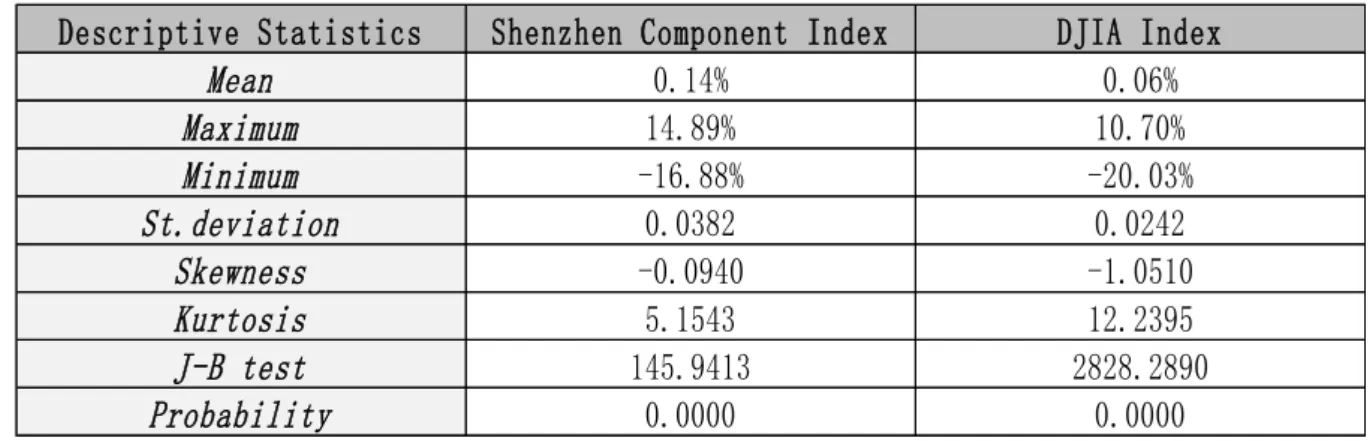
In Subchapter 2, some analysis of statistical features will be presented about selected stock index.
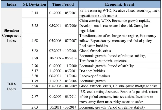
In Subchapter 3, the shock breaks will be identified respectively for returns of selected stock index.
In Subchapter 4, estimation models of conditional volatility will be created, as mention in Chapter 3. And the effect of volatility persistence or long memory will be analyzed.
In the last subchapter, in-sample analysis will be present for testing the quality of GARCH(1,1) model with and without dummy variables.
4.1 Description of Investigated Stock Markets
It is important to understand some information about the selected market, when we make a study for financial time series data. As the more information we know in a market, we can find the more structural break events easily.
In this subchapter, we will introduce the brief information about Chinese stock market and American stock market.
42
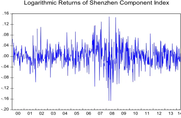
4.1.1 Features of Chinese Stock Market
There was a change in China, from centrally planned economy in 1950s ~ 1960s to more market orientated economy after 1980s. Currently, China is one of most significant participants in the global economy. And then Chinese emerging stock market also experienced a tremendous growth and development.
There are two Stock Exchanges in China, Shanghai Stock Exchange and Shenzhen Stock Exchange, which were established in 11/26/1990 and 12/01/1990 respectively. Generally, Shanghai Exchange is dominated by larger-cap companies, whereas in Shenzhen small joint-ventures and export-oriented company are listed. In addition, both exchanges are supervised by Chinese Securities Regulatory Committee or CRSC, which supervises new stock listing and daily trading activities.
In fact, it is proved that number of listed companies at both of Stock Exchanges grew up more than 100 times since 1990, and total market capitalization is far more than 500 billion USD. However, there was not a boom development in Chinese equity market before 2005. The reasons could be different, but the one main point should be, that Chinese currency was pegged to USD. When the foreign exchange regime was little liberalized, Chinese stock market started to experience a boom. A good example of this is that Shanghai Composite Index went up almost 130% and Shenzhen Composite Index even more as 197% in 2006.
Despite there is an amazing growth and development in Chinese equity market over the period of 20 years since 1990, the growth has been uneven and irregular. Especially in 2007~2008 global financial crisis, there is no denying that Chinese stock market experienced a dramatic decline. Therefore, we can conclude that Chinese stock market still remains in rather early stage of development, and it is necessary to reform and develop this inefficient market.
Furthermore, Chinese stock market has some unique, idiosyncratic features, which can be viewed in 6 aspects:
43
1. There are plenty of different classes of shares in China.
Chinese stock market actually consists of several sub-markets, with limited access and ability to buy stock and shares. Some of equity has limited access to either foreign or domestic investors, such as the restriction between A and B class.
To be more specific, On the one hand investments of A class shares are restricted only to domestic investors with rare exceptions. A class shares go public either on Shanghai or Shenzhen exchange, and they are denominated in not freely exchangeable RMB. On the other hand, foreign investors can trade B class shares, but these shares don‘t carry ownership rights in a company.
As we said about the sub-market in Chinese equity market, we have to mention H, N, L or S class shares, listed respectively in Honk Kong, New York, London and Singapore. What is more, most China‘s blue-chips are listed only on overseas exchanges, restricted only to foreign investors. This situation generates some structural drawbacks of Chinese stock market.
2. China market lacks true blue-chip stocks with high level of profitability. Besides it is dominant that the size gap between Chinese stock and others country‘s.
There are very few stocks that would fit the definition of ―blue-chip‖ trading on China‘s mainland exchanges. While most developed markets are dominated by a limited number of large-cap stocks, China‘s market is cramped by a multitude of small-cap stocks. Chinese companies are not operating on high level of profitability, instead of providing rather poor earnings, and low dividend yields. This feature allows for increased speculation and higher turnover for both investors and indexes, among other problems.
3. Chinese equity market is dominated by retail investors.
Holdings of institutions in China are not more than 20% of total market share, comparing to 40% in U.S.A, U.K or Japan. Moreover, holdings of foreign investors in China are not exceeding 2.5%, while in developed markets of U.S.A and Japan they own respectively 11% and 19%.
44
4. Expansion through the issuance of new shares is rather than the appreciation in value of existing stocks.
Since these existing shares generally do not experience sustained growth, often because of market manipulation, they tend to be smaller size stocks in China‘s market. As the result, the current structure is a major obstacle to the creation of viable index-related products in China.
5. To be honest, there is a serious speculation situation in Chinese equity market.
Speculation is a very widespread phenomenon throughout China‘s stock market in different kind of investors. Most of individual investors are fighting for financial survival in a risky investing environment, also institutional investors frequently engage in speculation. Furthermore, Chinese stock market is not really encouraging long-term investment strategies with stable yield, instead short term speculation strategies are use more.
At the same time, speculation in Chinese stock market provides liquidity and encourages trading activity. For example, the excessive stock market trading can be observed almost every trading day.
6. It is a phenomenon that the stock market is yet to be regulated strictly.
Chinese government strictly regulates initial public offerings. Normally it is desirable to have supervision over fairness of operations, but in China it is even more complicated. Size, allocation and development of stock market in china are fully under control of state. The government controls the quota for new listings that can be issued each year, even selects qualified issuers based on sector allocation.
4.1.2 Features of American Stock Market
The U.S. stock market started from New York Stock Exchange, which was established and began operating in 1811 by agent managers, according to the buttonwood agreement. At present the American stock market is mainly composed of the New York Stock Exchange, the NASDAQ Stock Exchange, American Stock Exchange and Over the Count market.