The Volatility Effect: Lower Risk without Lower Return

The Volatility Effect: Lower Risk without Lower Return

ERIMREPORT SERIES RESEARCH IN MANAGEMENT

ERIM Report Series reference number ERS-2007-044-F&A

Publication July 2007

Number of pages 19

Persistent paper URL

Email address corresponding author [email protected]

Address Erasmus Research Institute of Management (ERIM) RSM Erasmus University / Erasmus School of Economics Erasmus Universiteit Rotterdam

P.O.Box 1738

3000 DR Rotterdam, The Netherlands Phone: + 31 10 408 1182 Fax: + 31 10 408 9640 Email: [email protected] Internet: www.erim.eur.nl

Bibliographic data and classifications of all the ERIM reports are also available on the ERIM website: www.erim.eur.nl

ERASMUS RESEARCH INSTITUTE OF MANAGEMENT

REPORT SERIES

RESEARCH IN MANAGEMENT

A

K

Abstract We present empirical evidence that stocks with low volatility earn high risk-adjusted returns. The annual alpha spread of global low versus high volatility decile portfolios amounts to 12% over the 1986-2006 period. We also observe this volatility effect within the US, European and Japanese markets in isolation. Furthermore, we find that the volatility effect cannot be explained by other well-known effects such as value and size. Our results indicate that equity investors overpay for risky stocks. Possible explanations for this phenomenon include (i) leverage restrictions, (ii) inefficient two-step investment processes, and (iii) behavioral biases of private investors. In order to exploit the volatility effect in practice we argue that investors should include low risk stocks as a separate asset class in the strategic asset allocation phase of their investment process. Free Keywords alpha, strategic asset allocation, volatility, volatility effect, low risk stocks, CAPM, Fama-French

factors, international

Availability _{The ERIM Report Series is distributed through the following platforms:} Academic Repository at Erasmus University (DEAR), DEAR ERIM Series Portal

Social Science Research Network (SSRN), SSRN ERIM Series Webpage

Research Papers in Economics (REPEC), REPEC ERIM Series Webpage

Classifications _{The electronic versions of the papers in the ERIM report Series contain bibliographic metadata} by the following classification systems:

Library of Congress Classification, (LCC) LCC Webpage

Journal of Economic Literature, (JEL), JEL Webpage

ACM Computing Classification System CCS Webpage

The volatility effect: lower risk without lower return

David C. Blitz

Pim van Vliet

Abstract

We present empirical evidence that stocks with low volatility earn high risk-adjusted returns. The annual alpha spread of global low versus high volatility decile portfolios amounts to 12% over the 1986-2006 period. We also observe this volatility effect within the US, European and Japanese markets in isolation. Furthermore, we find that the volatility effect cannot be explained by other well-known effects such as value and size. Our results indicate that equity investors overpay for risky stocks. Possible explanations for this phenomenon include (i) leverage restrictions, (ii) inefficient two-step investment processes, and (iii) behavioral biases of private investors. In order to exploit the volatility effect in practice we argue that investors should include low risk stocks as a separate asset class in the strategic asset allocation phase of their investment process.

[Word count: approx. 5000]

First draft: December 2006 This version: April 2007

∗

David Blitz is Deputy Head of Quantitative Strategies at Robeco Asset Management in the Netherlands. Robeco Asset Management, Coolsingel 120, NL-3011 AG Rotterdam, The Netherlands. Email [email protected] and [email protected]. Pim van Vliet, PhD is Senior Researchers at Quantitative Strategies at Robeco Asset Management in the

Netherlands and is affiliated with the Erasmus School of Economics. We would like to thank Willem Jellema for programming assistance and appreciate the comments of Thierry Post, Gerben de Zwart and Laurens Swinkels. Any remaining errors are the authors’

responsibility.

I. Introduction

Efficient markets theory has been challenged by the finding that relatively simple investment strategies are found to generate statistically significantly higher returns than the market portfolio. Well-known examples are the value, size and momentum strategies, for which return premiums have been documented in US and international stock markets. Market efficiency is also challenged, however, if some simple

investment strategy generates a return similar to that of the market, but at a systematically lower level of risk.

An interesting study in this regard is the empirical analysis of the characteristics of minimum variance portfolios in Clarke, de Silva & Thorley (CST, 2006). These authors find that minimum variance portfolios, based on the 1,000 largest US stocks over the 1968-2005 period, achieve a volatility reduction of about 25%, whilst delivering comparable, or even higher, average returns than the market portfolio. We present a simple alternative approach to constructing portfolios with similar risk and return characteristics. Specifically, we create decile portfolios that are based on a straightforward ranking of stocks on their historical return volatility. Contrary to CST, we effectively only use the diagonal of the historical covariance matrix with this approach. We find that portfolios consisting of stocks with the lowest historical volatility are associated with Sharpe ratio improvements which are even larger than those in CST, and statistically significant positive alpha.

A related study in this regard is Ang, Hodrick, Xing & Zhang (AHXZ, 2006), who report that US stocks with high volatility earn abnormally low returns over the 1963-2000 period. These authors focus on a very short term (1 month) volatility measure, while in our study we concentrate on long-term (past 3 years) volatility, which implies a much lower portfolio turnover. Furthermore, we do not only find that high risk stocks are exceptionally unattractive, but also that low risk stocks are particularly attractive.

Ranking stocks on their historical volatility bears a resemblance to ranking stocks on their historical CAPM beta. Theoretically this follows from the fact that the beta of a stock is equal to its correlation with the market portfolio times its historical volatility and divided by the volatility of the market portfolio. Empirically we also observe that portfolios consisting of stocks with a low (high) volatility exhibit a low (high) beta as well. Since the earliest tests of the CAPM researchers have shown that the empirical relation between risk and return is too flat, e.g. Fama & MacBeth (1973). Similarly, others such as Black, Jensen & Scholes (1972) report that low beta stocks contain positive alpha. In their seminal paper, Fama and French (1992) show that beta does not predict return in the 1963-1990 period, especially after controlling for size. In our

sample we also find alpha for portfolios ranked on beta, but considerably less than for portfolios ranked on volatility.

Our main contributions to the existing literature are as follows. Firstly, we document a clear volatility effect: low risk stocks exhibit significantly higher risk-adjusted returns than the market portfolio, while high risk stocks significantly underperform on a risk-adjusted basis. Secondly, our findings are not restricted to the US stock market, but apply to both the global and regional stock markets. The alpha spread of the top versus bottom decile portfolio amounts to 12% per annum for our universe of global large-cap stocks over the 1986-2006 period. Thirdly, we compare the volatility effect with the classic size, value and momentum strategies and control for these effects. In order to disentangle the volatility effect from those other effects we use global and local Fama and French regressions and apply a double sorting methodology. We find that the volatility effect is in fact a separate effect, and of comparable magnitude. Fourthly, we provide possible explanations for the success of the strategy which include leverage restrictions, inefficient industry practice or behavioral biases among private investors, which all flatten the risk-return relation. Finally, we argue that benefiting from the low volatility effect in reality is not easy, as long as institutional investors do not include low risk stocks as a separate asset class in their strategic asset allocation process.

The remainder of this paper is organized as follows. In the following section we first describe our data and methodology. Our primary focus is on a universe of global large-cap stocks. Subsequently, we present results for the US, European and Japanese markets in isolation. In the next section we control for other cross-sectional effects, again tested on global and regional markets separately. This is followed by a discussion of possible explanations for the superior Sharpe ratios of low risk portfolios. We end with our conclusions and implications for investors.

II. Data and methodology

At the end of every month, starting in December 1985 and ending in January 2006, we identify all constituents of the FTSE World Developed index and take these as our universe for that particular month. This global large-cap universe consists of approximately 2,000 stocks on average; the actual number varying between about 1,500 and 2,400 over time. Many return irregularities are known to disappear or become significantly less pronounced when the universe is restricted to large-caps, which makes our choice of universe conservative.

Our data sources are Factset for FTSE index constituent and return data, Compustat for US fundamental data, Worldscope for non-US fundamental data and Thomson

Financial Datastream for short-term interest rate data. Short-term interest rates are used for converting local stock returns to local stock returns in excess of their local risk free return.i Return are log-transformed in order to make them additive over time. The log-transformed excess returns are used throughout our analysis for all return calculations.

At the end of each month we construct equally weightedii decile portfolios by ranking stocks on the past 3 year volatility of weekly returns. We also rank stocks on their book-to-market ratio (valuation), past 12 minus 1 month total return (momentum) and free float market value (size). For the volatility and size measures, stocks with the lowest scores are assigned to the top decile, while for the valuation and momentum strategies stocks with the highest factor scores are the preferred ones. Factor scores are compared directly across all stocks, without imposing sector or country

restrictions. As a result, the entire Japanese market may be unattractive on valuation at the height of the Japan bubble during the late eighties. We do control for regional effects by presenting results for the US, Europe and Japan markets in isolation. Portfolios are rebalanced with a monthly frequency and transaction costs are ignored throughout our analysis.

For each decile portfolio we calculate the return (in excess of the local risk-free return) over the month following portfolio formation. For the resulting time series of returns we calculate both the average, standard deviation and Sharpe ratio. In order to test for the statistical significance of the difference between two Sharpe ratios, we apply the Jobson & Korkie (1981) test with the Memmel (2003) correction. This test statistic is calculated according to the formula below and asymptotically follows a standard normal distribution.

[

]

Here SRi refers to the Sharpe ratio of portfolio i, ρi,j to the correlation between

portfolios i and j, and T to the number of observations.

We employ both a regression based methodology and a double-sorting methodology in order to disentangle the volatility effect from other effects. We use the portfolios sorted on size and book-to-market in order to construct global and regional Fama-French equivalent hedge factors. We define SMB (small-minus-big) and HML (high-minus-low book-to-market) as the return difference between the top 30% and the bottom 30% ranked stocks. By regressing the return of volatility sorted portfolios on these factors we control for possible systematic exposures to SMB and HML.

or book-to-market and subsequently on volatility within the size or book-to-market buckets. This is an empirically robust way to control for implicit loadings on these factors.

Fama-French adjusted alphas are estimated using the following equation:

Ri = αi + βi Rm + si SMB + hi HML + εi (2)

Here Ri is the return on decile portfolio i, Rm is the excess return on the global market

portfolio defined as the equally weighted average of all stocks, βi, si and hi are the

estimated factor exposures and αi is the Fama-French adjusted alpha. Single factor

CAPM-adjusted alphas are calculated by including only the Rm factor in the

regression. Statistical significance of the alphas is obtained in the straightforward manner from the regression.

III. Global results

Table 1 contains an overview of our main results on the full, global universe, for the decile portfolios ranked on past 3 year volatility. The top decile portfolio, which contains the low risk stocks, can be seen to generate returns which are slightly above average. In general, however, the relation between historical volatility and subsequent return appears to be rather weak, except for a large underperformance of the bottom decile portfolios, i.e. the high risk stocks. The difference in average return between the top and bottom decile portfolio equals 5.9%.

The results become more interesting when we shift to a risk-adjusted performance perspective instead of looking at straight returns. Ex post standard deviations can be seen to increase monotonically for the consecutive decile portfolios. The volatility of the top decile (D1) portfolio is only about two thirds that of the market portfolio. Note that this volatility reduction is even larger than the one found by CST (2006) for (US) minimum variance portfolios. At the other end we have the bottom decile (D10) portfolio, with a standard deviation which is almost double that of the market

portfolio. Combined with its low return, this results in a very low Sharpe ratio for the high risk stock portfolio. Because the other volatility decile portfolios exhibit

relatively small differences in average returns, their Sharpe ratios are driven primarily by the standard deviation in the denominator. One of our key findings is that the top decile of low risk stocks achieves a Sharpe ratios of 0.72, compared to a Sharpe ratio of only 0.40 for the market portfolio. This difference in Sharpe ratios is statistically significant at the 5% level. The Sharpe ratios show a steadily declining pattern across the volatility sorted portfolios, with the Sharpe ratio of the bottom decile portfolio being significantly lower (at the 5% level again) than the Sharpe ratio of the market

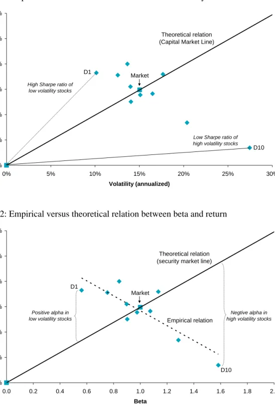
portfolio. Thus, we observe a clear relation between ex ante volatility and ex post risk-adjusted returns. A graphic illustration of these findings is given in Figure 1.

The next two rows contain the estimated beta and alpha from a CAPM style

regression of monthly decile portfolio returns on monthly returns of the market. This analysis shows that the low risk portfolio combines a very low beta of 0.56 with a positive alpha of 4.0% per annum, which is statistically significantly different from zero at the 1% significance level. The betas increase monotonically for the

consecutive decile portfolios, suggesting that volatility and beta are related risk measures. The bottom decile portfolio consisting of the highest risk stocks exhibits an estimated beta of 1.58 and a negative alpha of 8.0% per annum. This finding implies a negative relation between risk and return. The combined alpha spread for the low risk minus high risk portfolio amounts to 12.0%. A graphic illustration of these findings is given in Figure 2. The risk/return characteristics of the volatility sorted portfolios can be seen to be in clear violation of the theoretical (CAPM) security market line.

Panel B of Table 1 displays additional characteristics of the volatility decile portfolios. The first two rows contain a breakdown of the returns of the ten volatility portfolios with regard to up market months versus down market months. The low risk portfolios can be seen to underperform the market during up market months, while

outperforming the market during down market months. This behavior is consistent with the low beta of the low risk portfolios observed before. Importantly, the

underperformance during up months is considerably smaller than the outperformance during down months, although this effect is countered to some degree by the more frequent occurrence of up months (59%, versus 41% down months). The high risk portfolios exhibit precisely the opposite behavior: outperformance during up months, but not enough to offset the underperformance during down months. The third row in Panel B contains maximum drawdown statistics, defined as the maximum loss which an investor in these portfolios could have been confronted with (worst entry and worst exit moments). Just like the volatility of the low risk portfolios is only about two thirds that of the market, so are their maximum drawdowns, at 26% for the top decile portfolio versus over 38% for the market. As one would expect, the largest

drawdowns (exceeding 80%!) are experienced by the high risk portfolios.

In Table 2 we split the twenty year sample period into two ten year sub samples. The low volatility top decile portfolios exhibit the highest Sharpe ratios in both sub

periods. The alpha spread is significant in both the 1985-1995 and 1996-2005 periods. Furthermore, the strength of the effect does not appear to be diminishing over time, as the level and spread of the Sharpe ratios and alphas is in fact larger during the more recent sub period.

IV. Results by region

An inspection of the composition of the low risk portfolio over time suggests a pronounced ‘anti-bubble’ behavior. The strategy avoids the two main bubbles which occurred during our sample period: the Japan bubble in the late eighties and the TMT bubble in the late nineties. Avoiding these bubbles initially results in

underperformance, but after the bubbles burst the low risk portfolios tend to do particularly well. The underweight of Japan is in fact the most significant country bet of the strategy, with the US being the main beneficiary of the weight that needs to be redistributed. Note that during more recent years the underweight of Japan has gradually disappeared. At the sector level the strategy tends to systematically overweight sectors such as utilities and real estate, while a typical high risk sector such as IT is usually avoided by the strategy. For some other sectors the position taken by the strategy varies considerably over time. For example, the low risk portfolio initially contains a significant number of telecom stocks. During the TMT bubble stocks from the telecom sector are avoided however, only to make a

reappearance during the final years of our sample period.

In order to verify that the low risk anomaly is not the result of some systematic regional bets we now turn to the results on a regional basis. This analysis also sheds light on the robustness of the strategy. Panels A, B and C of Table 3 contain the main results for respectively the US, European and Japanese markets in isolation, structured in the same way as Table 1 for the global universe. The volatility effect turns out to be very persistent over the three regions, the regional results being similar to the results on a global basis.

For all three regions there is not much evidence of anomalous behavior of the volatility portfolios if we take a simple return perspective, except for a large underperformance of the bottom decile, i.e. the high risk stocks. For the US market we even find that the top decile of low risk stocks underperforms relative to the market. However, just like in the global analysis, the picture at the regional level changes dramatically if we take a risk-adjusted return perspective. All ex post standard deviations and betas increase monotonically for the consecutive volatility decile portfolios. Within each of the three regions the volatility of the top decile portfolios is only about 70% of the volatility of the market. The bottom decile

portfolios are consistently at the other extreme end, featuring standard deviations that are at least 50-100% higher than those of the market. Combined with the very low returns of these portfolios, this results in Sharpe ratios which are negative or close to zero. On the other hand, the top decile portfolios of low risk stocks exhibit Sharpe ratios which are well above those of the market. The Sharpe ratio improvement is biggest in Europe (Sharpe ratio of over 0.49 for the low risk portfolio versus 0.28 for the market), followed by Japan (0.34 versus 0.18) and lastly the US (0.58 versus 0.47).

For each region the Sharpe ratio of the high risk bottom decile portfolio is lower than that of the market with statistical significance at the 1% level.

The alpha spread is very consistent across the 3 main regions, varying from 10.2% for Europe to 13.8% for the US. The regional alpha spreads are of comparable magnitude as the alpha spread at the global level (12.0%), which implies that bottom-up regional allocation is not the key driver for the global results. The alpha spreads are

statistically significantly different from zero at the 5% level for the US and Japan, and even at the 1% level for Europe.

V. Controlling for other effects

How does the volatility effect relate to other effects, which have been documented in previous research? For example, could it be that the low-volatility portfolio contains a high proportion of value stocks, and that as a result of this it is simply capturing the value premium? And how does the magnitude of the volatility effect compare to classic effects such as value, size and momentum?

In order to answer these questions we first turn to Table 4, which contains the same statistics as we saw before for the low volatility portfolios, but now for the classic value, momentum and size strategies (as defined earlier). Consistent with previous research, we find that the top deciles of the value and momentum strategies

outperform relative to the equally weighted universe, while the bottom deciles underperform. However, we find little evidence of a size effect within our sample of FTSE world developed index constituents.

Interestingly, the low volatility top decile portfolio delivers a higher return per unit of risk (Sharpe ratio) than each individual value, momentum and size decile portfolio. From an alpha perspective the volatility effect ranks second out of four, only the momentum effect being somewhat stronger in our sample. Based on this analysis we conclude that the volatility effect holds out well in terms of magnitude, and thus economic relevance, in comparison to other classic effects.

A comparison of the characteristics of the volatility decile portfolios to the other decile portfolios suggests that the low volatility effect does indeed constitute a separate effect. For example, the top decile portfolios on value, size and momentum exhibit a volatility which is higher than that of the market, while the volatility of the low volatility portfolio is only about two thirds of that of the market. Also, the betas of the value, size and momentum top decile portfolios are close to, or even above 1, while the low volatility top decile portfolio exhibits a beta of only 0.56. These very

different characteristics suggest that the low volatility effect is a distinct effect, and not some classic effect in disguise.

Table 5 further separates the volatility effect from the other effects by means of Fama-French (FF) regressions. Panel A shows the alphas by correcting for value and size using a global Fama-French factor model. We find that one third of the global alpha spread of 12.0% can be attributed to size and value exposures. The 8.1% alpha which remains is thus not related to value and/or size and is left unexplained. Panel B shows the results of similar analyses at the regional level, based on local Fama-French regressions. The FF-adjustment has the biggest impact for the US, where the alpha drops from 13.8% to 7.0%. For Europe the alpha is lowered to 7.4% from 10.2%. The alpha is least affected for Japan, at 9.8% versus 10.5%. From these results we can conclude that the volatility effect is reduced, but does not disappear after applying the FF-adjustment.

The FF-adjustment is based on a single regression, which is applied ex post to the time series of returns. Thus, the factor exposures are estimated and assumed to be constant over time. An alternative way to disentangle the volatility effect from other cross-sectional effect is to apply a double sorting approach. This is a robust, non-parametric technique which enables us to systematically neutralize other effects ex ante. Panel A of Table 6 contains the results of a double sort on value followed by volatility. Every month stocks are first grouped into five quintiles based on value (book-to-market). Next we create decile portfolios based on volatility within each of these value quintiles. Finally, a value neutral top decile volatility portfolio is

constructed by combining the five top decile volatility portfolios from within each value quintile (and similarly for the other decile portfolios). Panels B contains similar results for a double sort on size followed by volatility, and Panel C for a double sort on momentum followed by volatility.

The volatility effect turns out to be robust to the ex ante factor neutralizations of the double sorts. The global (CAPM-)alpha remains at 8.9% or higher, and the alpha for the US at 9.5% or higher. Only for Europe we find that the alpha drops to 6.4%, in case of the momentum double sort, and for Japan to 6.6%, in case of the value double sort. Again we conclude that classic effects at most explain only part of the volatility effect.

VI. Robustness tests

The volatility effect is robust to a different measurement period for volatility. Panel A of Table 7 shows the CAPM-alphas of decile portfolios based on 1 year instead of 3 year weekly historical return volatility. The top versus bottom decile alpha spread is

slightly lower in a global context (11.2% versus 12.0%), but can be seen to increase somewhat for both the US and Europe. Only for Japan the alpha spread drops by a relatively large amount, from 10.5% to 7.1%.

We also compare the volatility effect with the classic beta effect, as described in the introduction. Contrary to volatilities, estimated betas are sensitive to the choice of the market portfolio. Beta can for example be estimated relative to a global index, but also relative to a regional index. This is an important empirical issue. For example, the Japanese market has shown a low correlation with the global stock market, which ceteris paribus results in lower estimated betas relative to a global index for all Japanese stocks. In order to avoid this issue and in order to have comparable results with other (US) studies, we concentrate on beta sorted portfolios at the regional level. In Panel B of Table 7 we compare the CAPM alphas of portfolios sorted on 3 year historical volatility with those of portfolios sorted on 3 year historical beta, again calculated using weekly return data. For each region we find a clear beta effect. However, the alpha spreads of the beta sorted portfolios are about 3-7 percent smaller for each region, and the alpha patterns are more irregular than those for the volatility sorted portfolios. Therefore, we conclude that the volatility effect is a stronger and less ambiguously defined effect than the beta effect.

Further evidence supporting this conclusion is given in Panel C of Table 7, which contains results of double sorting first on beta and then on volatility, similar in set-up as the double sorts described before. Although in this way the alpha is partly

subsumed, about 7% remains for Europe and Japan and 4% for the US. Thus, even within groups of stocks with similar betas, sorting stocks on volatility helps to capture additional alpha. Thus, the volatility effect cannot be explained by the classic beta effect. Furthermore, this finding suggests that both the idiosyncratic part and systematic part of volatility are mispriced.

VII. Possible explanations

In this section we discuss several possible explanations for the volatility effect as documented in this paper.

Firstly, leverage is needed in order to take full advantage of the attractive absolute returns of low risk stocks. In theory this is quite straightforward, but in practice many investors are either not allowed or unwilling to actually apply leverage, especially on the scale needed for exploiting this effect. For example, if a low risk stock portfolio has a volatility which is two-thirds of that of the market, 50% leverage needs to be applied in order to obtain the same level of volatility as the market. As a result, the opportunity which is presented by low risk stocks is not easily arbitraged away.

Borrowing restrictions were already identified by Black (1972) as an argument for the relatively good performance of low beta stocks.

Leveraged buyout (LBO) private equity funds might constitute a notable exception in this regard, because a key source of return of LBO funds is the application of leverage to the balance sheets of the companies in which they invest. Thus, the success of LBO private equity investing may, to some degree, be related to the high risk-adjusted returns of low risk stocks. Pure equity investors may be facing practical limitations with regard to leverage, but we want to stress that leverage can be created relatively easily within a balanced portfolio which contains bonds and/or cash next to stocks. Black (1993) already suggested an increased allocation to low risk stocks as an alternative to a given allocation to the market portfolio. For example, instead of investing 50% in traditional stocks and 50% in bonds, an investor might decide to invest 70% in low risk stocks and 30% in bonds. However, this requires that low risk stocks are included as a separate asset class in the strategic asset allocation process of investors. This is not the case in practice however. At least, not yet.

Secondly, the volatility effect could be the result of an inefficient decentralized investment approach. For example, in the professional investment industry it is common practice that first the CIO or an investment committee makes the asset allocation decision, and in a next stage this capital is allocated to managers who buy securities within the different asset classes. Binsbergen et. al (2007) demonstrate that this approach may result in inefficient portfolios. The problem with benchmark driven investing is that asset managers have an incentive to tilt towards high beta and/or high volatility stocks, as this is a relatively simple way for asset managers to generate above average returns, assuming the CAPM holds at least partially. As a result, these high risk stocks may become overpriced, whilst low risk stocks may become

underpriced, which is consistent with the return patterns which we document in this paper. Furthermore, new money tends to flow towards asset classes that do well, and within such asset classes to managers with above average performance. This suggests that for a profit-maximizing asset manager outperformance in up markets may be more desirable than outperformance in down markets. Asset managers may thus be willing to overpay for stocks which outperform in up markets, which tend to be high volatility stocks, and underpay for stocks which outperform in down markets, which tend to be low volatility stocks. In sum, the twin desire for outperformance and cash flow of asset managers may result in inefficient portfolios. A solution may be to integrate the two stage process by giving the asset managers one single benchmark, for example the fund specific liabilities, plus a risk budget to deviate.

Thirdly, the volatility effect may be caused by behavioral biases among private

investors. Behavioral portfolio theory describes that private investors think in terms of a two-layer portfolio. Shefrin & Statman (2000) identify a low aspiration layer which

is designed to avoid poverty, and a high aspiration layer which is designed for a shot at riches. Suppose that private investors make a rational risk-averse choice in the asset allocation decision (first layer), but become risk-neutral or even risk-seeking within a certain specific asset class (second layer). In this case, investors will overpay for risky stocks which are perceived to be similar to lottery tickets. In this perception, buying many stocks destroys upside potential, while buying a few volatile stocks (wish I had bought Microsoft in the eighties) leaves upside potential intact. This way of thinking is consistent with the finding that most private investors only hold about 1-5 stocks in their portfolio, thereby largely ignoring the diversification benefits that are available within the equity market. Deviations from risk-averse behavior of investors may cause high-risk stocks to be overpriced and low-risk stocks to be underpriced.

VIII. Conclusion and implications

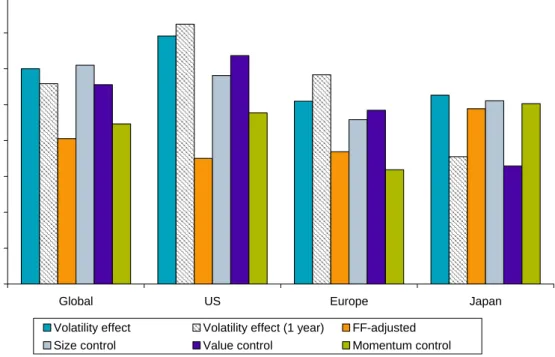
In this paper we have shown that stocks with low historical volatility exhibit superior risk adjusted returns, both in terms of Sharpe ratios and in terms of CAPM alphas. The volatility effect is similar in size compared to classic effects such as value, size and momentum, and largely remains after Fama-French adjustments and double sorts. A summary of the main results is given in Figure 3. Compared to Clarke et al. (2006), who find significantly lower risk and superior Sharpe ratios for US minimum variance portfolios, our results are stronger, while our approach is easier. Our results are

consistent with Ang et al. (2006), who document a large negative alpha for US stocks with high idiosyncratic volatility. However, our results are more symmetric, and based on 3 year instead of 1 month historical volatility, which implies a much lower portfolio turnover.

The volatility effect is particularly strong in a global setting, with a low versus high volatility alpha spread of 12%. The results remain strong however at the regional level (>10%). The low volatility strategy is characterized by relatively small drawdowns, a low beta, outperformance in down markets and underperformance in up markets and anti-bubble behavior. Possible explanations for the success of the strategy include the practical difficulties with arbitraging the effect away due to a need for applying significant leverage, inefficient industry practice or behavioral biases among private investors, which all flatten the risk-return relation.

Exploiting the volatility effect is not easy for benchmark driven equity investors who are facing a relative return objective and are either not allowed or willing to apply leverage. However, for investors interested in high Sharpe ratio investment opportunities such as pension funds, it may be much easier to benefit from the volatility effect, by applying leverage within their asset mix. These investors could simply decide to shift from a given allocation to traditional stocks to a higher

allocation to low risk stocks, by reducing the weight of bonds. In order for this option to be taken adequately into account it is essential to include the decision to invest in low risk stocks in the strategic asset allocation process. Therefore, we recommend that absolute return investors distinguish between low risk, high risk and traditional stocks as separate asset classes, just like they distinguish between value versus growth stocks and large-cap versus small-cap stocks in their strategic asset allocation decision making.

References

Ang, Andrew, Robert J. Hodrick, Yuhang Xing & Xiaoyan Zhang (2006), The cross-section of volatility and expected returns, Journal of Finance, Vol. LXI, No. 1, February 2006, pp. 259-299

Binsbergen, J.H. van, R. Koijen and Michael W. Brandt (2007), Optimal

Decentralized Investment Management, NBER 12144, Forthcoming in the Journal of Finance 2007

Black, Fischer (1972), Capital Market Equilibrium with Restricted Borrowing, Journal of Business, 45, pp. 444-455

Black, Fischer, Michael C. Jensen, and Myron Scholes (1972), The capital asset pricing model: some empirical tests, Studies in the theory of capital markets (Praeger)

Black, Fischer (1993), Beta and Return: Announcements of the ‘Death of Beta’ seem Premature, Journal of Portfolio Management Fall 1993, pp. 11-18

Clarke, Roger, Harindra de Silva & Steven Thorley (2006), Minimum-variance portfolios in the US equity market, Journal of Portfolio Management, Fall 2006, pp.10-24

Fama, Eugene F., and Kenneth R. French (1992), The cross-section of expected stock returns, Journal of Finance 47, pp. 427-465

Fama, Eugene F., and James D. MacBeth (1973), Risk, return and equilibrium: Empirical tests, Journal of Political Economy 71, pp. 43-66

Jobson, J. D. & Korkie, B. M. (1981), Performance Hypothesis Testing with the Sharpe and Treynor Measures, Journal of Finance 36, pp. 889-908.

Memmel, C. (2003), Performance Hypothesis Testing with the Sharpe Ratio, Finance Letters 1, pp. 21-23.

Shefrin, Hersh and Meir Statman 2000, Behavioral Portfolio Theory, The Journal of Financial and Quantitative Analysis, Vol. 35, No. 2 pp. 127-151

i

Note that using these returns is equivalent to assuming that first all currency risk is hedged to

whichever base currency, and next converting these currency hedged stock returns to excess returns, by subtracting the risk free return of the chosen base currency.

ii

All results presented in this paper are based on equally weighted portfolios. For cap-weighted portfolios we found similar results, but these are not presented for the sake of brevity.

Table 1: Main results global decile portfolios based on historical volatility D1 D2 D3 D4 D5 D6 D7 D8 D9 D10 D1-10 Univ Excess return 7.3% 7.1% 8.0% 6.2% 5.0% 5.6% 5.6% 7.2% 3.4% 1.4% 5.9% 6.0% Standard deviation 10.1% 12.6% 13.6% 14.0% 14.0% 15.1% 16.5% 17.7% 20.4% 27.5% 23.7% 15.0% Sharpe ratio 0.72 0.57 0.59 0.44 0.36 0.37 0.34 0.41 0.17 0.05 0.40 (t-value) 2.2 1.6 2.0 0.8 -0.6 -0.5 -1.1 0. -2.8 -2.7 -1.02 -0.4% -0.3% -0.7% -4.3% -8.0% -0.4 -0.3 -1.0 0. -2.9 -2.6 -1.1% -0.7% -0.3% -0.3% -0.4% -0.2% -2.5% -0.4% -0.5% -1.5% -2.9% -26% -32% -33% -36% -46% -41% -40% -43% -67% -86% -38% -2.4% -1.2% -0.4% -2.2% -3.6% -0.0% -1.0% -6.9% -14.2% -0.0% -2.6 -2.1 -2.6 -1.32 -3.2% -4.3% -10.6% -2.6 -1.9 -2.3 -0.0% -0.00 -0.2 -1.8 -2.7 -1.7 -2.7 -0.85 -1.6% -3.0% -2.6% -7.3% -0.0% -1.8 -2.9 -1.5 -2.7 -2.3% -0.07 -0.3 -0.7 -1.7 -2.6 -0.81 -0.3% -0.8% -2.9% -7.7% -0.0% -0.2 -0.7 -1.7 -2.8 2 -Beta 0.56 0.75 0.84 0.90 0.90 0.98 1.07 1.13 1.29 1.58 1.00 Alpha 4.0% 2.6% 3.0% 0.9% 0.4% 12.0% -(t-value) 3.1 2.2 2.6 1.0 4 3.0 -D1 D2 D3 D4 D5 D6 D7 D8 D9 D10 D1-10 Univ Return up 0.2% 0.5% 0.6% 1.4% 0.0% Return down 1.8% 1.2% 0.9% 0.5% 0.4% 0.2% 4.8% 0.0% Max drawdown

-Panel A: Decile portfolios based on historical return volatility

Panel B: Risk analysis of portfolios based on historical volatility

0.4% 6.5% D1 D2 D3 D4 D5 D6 D7 D8 D9 D10 D1-D10 Univ Excess return 8.7% 8.1% 9.0% 8.0% 8.5% 8.1% 6.9% 9.0% 3.9% 1.0% 7.7% 7.5% Standard deviation 8.0% 10.3% 11.5% 11.9% 13.3% 14.2% 15.4% 16.8% 21.5% 33.0% 30.6% 14.3% Sharpe ratio 1.09 0.79 0.78 0.67 0.64 0.57 0.45 0.53 0.18 0.03 0.53 Alpha 5.7% 3.5% 3.6% 2.0% 1.7% 0.8% 0.4% 19.8%

Panel A: Jan 1986 through Dec 1995

Panel B: Jan 1996 through Jan 2006

-Beta 0.45 0.70 0.82 0.86 0.94 0.95 1.01 1.16 1.39 1.77 1.00 Alpha 3.3% 1.9% 1.5% 1.9% 0.7% 1.1% 1.4% 13.8% 0.0% (t-value) 1.6 1.3 1.1 1.4 0.5 1.3 1.3 2.3 -D1 D2 D3 D4 D5 D6 D7 D8 D9 D10 D1-10 Univ Excess return 6.0% 6.9% 6.3% 6.8% 5.2% 4.7% 3.5% 2.4% 3.7% 6.0% 4.9% Standard deviation 12.4% 14.2% 15.1% 16.9% 17.2% 17.8% 19.0% 20.2% 23.7% 28.7% 21.6% 17.5% Sharpe ratio 0.49 0.49 0.42 0.40 0.31 0.27 0.19 0.12 0.16 0.28 (t-value) 1.9 2.1 1.8 1.8 0.5 -Beta 0.64 0.74 0.82 0.93 0.94 0.98 1.06 1.12 1.29 1.49 1.00 Alpha 2.9% 3.3% 2.4% 2.3% 0.7% 0.0% 10.2% (t-value) 2.4 2.6 2.1 2.1 0.6 0.0 2.9 -D1 D2 D3 D4 D5 D6 D7 D8 D9 D10 D1-10 Univ Excess return 5.1% 5.1% 3.0% 4.6% 4.8% 4.2% 4.7% 3.5% 1.6% 7.5% 3.8% Standard deviation 15.2% 18.0% 19.6% 20.1% 21.5% 22.3% 23.2% 25.3% 27.1% 33.0% 25.5% 21.5% Sharpe ratio 0.34 0.28 0.15 0.23 0.22 0.19 0.20 0.14 0.06 0.18 (t-value) 1.3 1.3 0.9 0.9 0.3 0.6 -Beta 0.61 0.78 0.87 0.91 0.98 1.02 1.06 1.15 1.21 1.42 1.00 Alpha 2.8% 2.1% 1.2% 1.1% 0.4% 0.7% 10.5% (t-value) 1.6 1.5 1.0 1.0 0.4 0.7 2.5

-Panel A: Main results US

Panel B: Main results Europe

Panel C: Main results Japan

Table 2: Sub period analysis of global decile portfolios based on historical volatility

D1 D2 D3 D4 D5 D6 D7 D8 D9 D10 D1-D10 Univ

Excess return 5.9% 6.1% 7.0% 4.4% 1.5% 3.0% 4.4% 5.4% 2.9% 1.7% 4.1% 4.4% Standard deviation 11.9% 14.5% 15.5% 15.8% 14.8% 15.9% 17.5% 18.5% 19.3% 20.6% 13.7% 15.8% Sharpe ratio 0.49 0.42 0.45 0.28 0.10 0.19 0.25 0.29 0.15 0.08 0.28 Alpha 2.9% 2.3% 2.9% 0.1%

Table 3: Regional results

D1 D2 D3 D4 D5 D6 D7 D8 D9 D10 D1-10 Univ

Excess return 6.9% 7.6% 8.1% 8.9% 8.3% 8.9% 9.6% 6.3% 7.0% 3.8% 3.1% 8.1% Standard deviation 12.0% 13.7% 15.4% 15.9% 17.0% 16.7% 18.0% 20.7% 25.8% 36.5% 35.0% 17.1% Sharpe ratio 0.58 0.56 0.53 0.56 0.49 0.53 0.53 0.30 0.27 0.10 0.47 (t-value) 0.5 0.7 0.6 0.9 0.2 1.0 0.9

Table 4: Comparison with other investment strategies D1 D2 D3 D4 D5 D6 D7 D8 D9 D10 D1-10 Univ Excess return 5.4% 7.6% 6.3% 6.7% 5.8% 5.5% 6.5% 5.6% 4.4% 4.5% 0.9% 6.0% Standard deviation 18.5% 15.6% 16.1% 15.9% 15.9% 15.8% 15.3% 14.7% 15.2% 15.2% 13.4% 15.0% Sharpe ratio 0.29 0.49 0.39 0.42 0.36 0.35 0.43 0.38 0.29 0.30 0.40 (t-value) -1.0 -0.1 -0.7 -1.0 0. -0.3 -1.3 -0.9 -1.1% -0.4% -0.6% -0.1% -1.2% -0.9% -0.3% -0.0% -0.6 -0.6 -0.9 0. -0.1 -1.0 -0.6 -0.1 -1.5 -1.4 -2.6 -2.2 -1.8 -2.3 -1.0% -1.0% -2.0% -2.0% -1.9% -3.9% -0.0% -1.4 -1.3 -2.8 -2.2 -1.6 -2.1 -0.5 -2.1 -3.1 -3.0 -2.5 -0.53 -0.2% -1.6% -3.6% -5.2% -7.9% -0.0% -0.3 -2.1 -3.4 -3.1 -2.3 -0.4% -0.3% -0.7% -4.3% -8.0% -0.8% -0.3% -0.6% -2.9% -5.4% -3.2% -4.3% -10.6% -2.8% -2.9% -5.7% -1.6% -3.0% -2.6% -7.3% -0.5% -2.3% -3.8% -2.1% -4.2% -0.3% -0.8% -2.9% -7.7% -0.5% -1.7% -7.7% 1.1 0.6 5 -Beta 1.10 0.98 1.03 1.03 1.04 1.03 0.98 0.95 0.95 0.90 0.20 1.00 Alpha 1.7% 0.1% 0.6% 0.7% (t-value) 1.5 0.1 0.8 8 -D1 D2 D3 D4 D5 D6 D7 D8 D9 D10 D1-10 Univ Excess return 9.3% 9.5% 8.8% 7.3% 4.8% 4.8% 3.8% 3.9% 4.0% 2.0% 7.3% 6.0% Standard deviation 20.0% 16.1% 15.0% 14.4% 15.0% 15.2% 15.0% 15.5% 15.9% 16.8% 14.4% 15.0% Sharpe ratio 0.46 0.59 0.59 0.50 0.32 0.32 0.25 0.25 0.25 0.12 0.40 (t-value) 0.6 2.4 2.6 1.8 -Beta 1.20 1.02 0.95 0.93 0.97 0.98 0.98 0.99 0.99 0.98 0.22 1.00 Alpha 2.1% 3.4% 3.1% 1.7% 6.0% (t-value) 1.1 3.1 3.3 2.2 1.9 -D1 D2 D3 D4 D5 D6 D7 D8 D9 D10 D1-10 Univ Excess return 12.1% 8.6% 8.7% 6.1% 6.0% 5.1% 3.9% 2.5% 1.8% 0.9% 11.2% 5.9% Standard deviation 17.5% 14.9% 13.7% 13.7% 13.6% 14.0% 14.5% 16.4% 19.4% 27.0% 24.0% 15.0% Sharpe ratio 0.69 0.58 0.63 0.44 0.44 0.36 0.27 0.15 0.09 0.03 0.39 (t-value) 2.0 1.7 2.5 0.7 0.9 -Beta 0.96 0.89 0.85 0.87 0.88 0.90 0.94 1.05 1.19 1.49 1.00 Alpha 6.5% 3.4% 3.7% 1.0% 0.9% 14.3% (t-value) 2.9 2.3 3.3 1.0 1.2 2.8

-Panel B: Decile portfolios based on Value (book-to-market)

Panel C: Decile portfolios based on Momentum (12-1M) Panel A: Decile portfolios based on Size (market capitalization)

0.4% 12.0% FF-Alpha 2.8% 1.3% 1.8% 0.3% 1.2% 8.1% D1 D2 D3 D4 D5 D6 D7 D8 D9 D10 D1-10 US 3.3% 1.9% 1.5% 1.9% 0.7% 1.1% 1.4% 13.8% FF-Alpha 1.3% 0.6% 0.2% 1.0% 0.3% 0.8% 1.0% 7.0% Europe 2.9% 3.3% 2.4% 2.3% 0.7% 0.0% 10.2% FF-Alpha 3.2% 3.0% 1.9% 1.9% 0.3% 7.4% Japan 2.8% 2.1% 1.2% 1.1% 0.4% 0.7% 10.5% FF-Alpha 2.1% 1.9% 0.1% 1.2% 0.5% 0.0% 0.7% 9.8%

Panel A: Fama-French corrected alphas

Panel B: Regional Fama-French corrected alphas

Table 5: Global and regional Fama-French corrected alphas

D1 D2 D3 D4 D5 D6 D7 D8 D9 D10 D1-10 Global Alpha 4.0% 2.6% 3.0% 0.9%

Table 6: Double sorted results D1 D2 D3 D4 D5 D6 D7 D8 D9 D10 D1-10 Global 3.5% 3.0% 2.5% 0.6% 0.4% -0.1% -1.1% -0.6% -3.1% -7.6% -0.5% -0.9% -5.7% -9.4% -0.6% -3.0% -2.1% -7.3% -0.8% -1.8% -5.3% -1.5% -1.6% -2.9% -8.3% -0.7% -2.6% -6.0% -7.8% -1.4% -1.2% -1.0% -3.4% -6.5% -0.2% -1.0% -8.7% -1.1% -0.5% -2.0% -6.0% -0.6% -0.3% -0.9% -4.2% -6.5% -1.3% -1.2% -2.5% -4.7% -0.7% -2.3% -7.2% -1.1% -0.5% -0.3% -1.4% -8.1% -4.0% -5.3% -10.4% -0.7% -1.5% -1.7% -8.7% -0.5% -0.2% -2.6% -6.3% -3.2% -4.3% -10.6% -3.2% -4.2% -8.1% -1.6% -3.0% -2.6% -7.3% -0.7% -1.8% -4.1% -5.9% -0.3% -0.8% -2.9% -7.7% -1.4% -5.3% -5.3% -0.5% -2.9% -2.4% -2.1% -1.3% -0.2% -2.9% -4.8% -1.1% -0.1% -0.3% -2.1% -4.9% 11.1% US 3.4% 1.7% 2.3% 2.4% 1.2% 0.3% 12.7% Europe 2.4% 3.7% 2.7% 0.9% 0.7% 0.1% 9.7% Japan 1.3% 0.5% 0.5% 0.8% 1.0% 0.2% 0.7% 6.6% D1 D2 D3 D4 D5 D6 D7 D8 D9 D10 D1-10 Global 3.9% 2.4% 2.6% 1.6% 0.4% 0.7% 12.2% US 3.8% 1.6% 1.6% 2.3% 1.0% 1.3% 11.6% Europe 2.7% 3.5% 1.4% 0.9% 2.6% 9.2% Japan 1.5% 2.4% 0.3% 1.6% 0.2% 0.9% 0.5% 10.2% D1 D2 D3 D4 D5 D6 D7 D8 D9 D10 D1-10 Global 2.9% 2.5% 1.5% 0.7% 0.3% 0.3% 8.9% US 3.0% 2.0% 1.8% 1.6% 0.5% 9.5% Europe 1.7% 3.0% 1.3% 0.2% 0.7% 1.1% 6.4% Japan 2.8% 1.3% 0.8% 0.7% 1.0% 0.7% 0.4% 10.1%

Panel C: Alpha from double sort on momentum (12-1M) and volatilty (past 3 years) Panel B: Alpha from double sort on size (market capitalization) and volatilty (past 3 years)

Panel A: Alpha from double sort on value (book-to-market) and volatilty (past 3 years)

0.1% 11.2% US 4.1% 0.3% 2.3% 2.0% 1.5% 1.6% 1.8% 14.5% Europe 3.0% 2.7% 1.3% 1.8% 0.7% 0.0% 11.7% Japan 0.8% 1.3% 2.1% 0.2% 1.3% 0.2% 7.1% D1 D2 D3 D4 D5 D6 D7 D8 D9 D10 D1-10 US volatility 3.3% 1.9% 1.5% 1.9% 0.7% 1.1% 1.4% 13.8% US beta 1.2% 1.7% 1.8% 2.5% 0.2% 1.5% 1.2% 9.3% Europe volatility 2.9% 3.3% 2.4% 2.3% 0.7% 0.0% 10.2% Europe beta 1.5% 2.4% 2.8% 0.9% 1.4% 0.7% 7.5% Japan volatility 2.8% 2.1% 1.2% 1.1% 0.4% 0.7% 10.5% Japan beta 1.2% 1.1% 1.5% 0.7% 1.3% 1.3% 0.7% 3.8% D1 D2 D3 D4 D5 D6 D7 D8 D9 D10 D1-10 US 2.3% 0.8% 0.8% 0.6% 0.6% 0.2% 4.4% Europe 2.3% 1.4% 1.5% 1.5% 0.0% 0.7% 7.1% Japan 2.0% 1.8% 1.6% 0.1% 1.0% 6.9%

Panel C: Alpha from double sort on beta (past 3 years) and volatilty (past 3 years) Panel B: CAPM-alpha for regional decile portfolios sorted on volatility versus beta Panel A: CAPM-alpha for regional decile portfolios sorted on 1 year (instead of 3 year) volatility

Table 7: Robustness tests

D1 D2 D3 D4 D5 D6 D7 D8 D9 D10 D1-10 Global 3.1% 2.0% 1.8% 1.4%

Figure 1: Empirical versus theoretical relation between volatility and return 0% 2% 4% 6% 8% 10% 12% 0% 5% 10% 15% 20% 25% 30% Volatility (annualized) Ex cess retu rn (a nn ualized) Theoretical relation (Capital Market Line)

Low Sharpe ratio of high volatility stocks

D1

D10 Market

High Sharpe ratio of low volatility stocks

Figure 2: Empirical versus theoretical relation between beta and return

0% 2% 4% 6% 8% 10% 12% 0.0 0.2 0.4 0.6 0.8 1.0 1.2 1.4 1.6 1.8 2.0 Beta Ex cess retu rn (a nn ualized) Theoretical relation (security market line)

Empirical relation D1

D10 Market

Positive alpha in low volatility stocks

Negtive alpha in high volatility stocks

Figure 3: Summary of alpha findings 0% 2% 4% 6% 8% 10% 12% 14% 16%

Global US Europe Japan

To p mi nu s b o tt om d e ci le a lph a sp re a d

Volatility effect Volatility effect (1 year) FF-adjusted Size control Value control Momentum control

Publications in the Report Series Research

in Management

2007

Revisiting Uncovered Interest Rate Parity: Switching Between UIP and the Random Walk

Ronald Huisman and Ronald Mahieu ERS-2007-001-F&A

http://hdl.handle.net/1765/8288

Hourly Electricity Prices in Day-Ahead Markets

Ronald Huisman, Christian Huurman and Ronald Mahieu ERS-2007-002-F&A

http://hdl.handle.net/1765/8289

Do Exchange Rates Move in Line with Uncovered Interest Parity?

Ronald Huisman, Ronald Mahieu and Arjen Mulder ERS-2007-012-F&A

http://hdl.handle.net/1765/8993

Hedging Exposure to Electricity Price Risk in a Value at Risk Framework

Ronald Huisman, Ronald Mahieu and Felix Schlichter ERS-2007-013-F&A

http://hdl.handle.net/1765/8995

Corporate Governance and Acquisitions: Acquirer Wealth Effects in the Netherlands

Abe de Jong, Marieke van der Poel and Michiel Wolfswinkel ERS-2007-016-F&A

http://hdl.handle.net/1765/9403

The Effect of Monetary Policy on Exchange Rates during Currency Crises; The Role of Debt, Institutions and Financial Openness

Sylvester C.W. Eijffinger and Benedikt Goderis ERS-2007-022-F&A

http://hdl.handle.net/1765/9725

Do Private Equity Investors Take Firms Private for Different Reasons?

Jana P. Fidrmuc, Peter Roosenboom and Dick van Dijk ERS-2007-028-F&A

http://hdl.handle.net/1765/10070

The Influence of Temperature on Spike Probability in Day-Ahead Power Prices

Ronald Huisman ERS-2007-039-F&A

http://hdl.handle.net/1765/10179

Costs and Recovery Rates in the Dutch Liquidation-Based Bankruptcy System

Oscar Couwenberg and Abe de Jong ERS-2007-041-F&A

The Volatility Effect: Lower Risk without Lower Return

David C. Blitz and Pim van Vliet ERS-2007-044-F&A

∗

A complete overview of the ERIM Report Series Research in Management:

https://ep.eur.nl/handle/1765/1 ERIM Research Programs:

LIS Business Processes, Logistics and Information Systems ORG Organizing for Performance

MKT Marketing

F&A Finance and Accounting STR Strategy and Entrepreneurship