Scientific Background on the Sveriges Riksbank Prize in Economic Sciences in Memory of Alfred Nobel 2013
U N D E R S TA N D I N G A S S E T P R I C E S
compiled by the Economic Sciences Prize Committee of the Royal Swedish Academy of Sciences
THE ROYAL SWEDISH ACADEMY OF SCIENCEShas as its aim to promote the sciences and strengthen their influence in society.
BOX 50005 (LILLA FRESCATIVÄGEN 4 A), SE-104 05 STOCKHOLM, SWEDEN TEL +46 8 673 95 00, FAX +46 8 15 56 70, [email protected] HTTP://KVA.SE
UNDERSTANDING ASSET PRICES
1.
Introduction
The behavior of asset prices is essential for many important decisions, not only for professional investors but also for most people in their daily life. The choice between saving in the form of cash, bank deposits or stocks, or perhaps a single-family house, depends on what one thinks of the risks and returns associated with these different forms of saving. Asset prices are also of fundamental importance for the macroeconomy because they provide crucial information for key economic decisions regarding physical investments and consumption. While prices of financial assets often seem to reflect fundamental values, history provides striking examples to the contrary, in events commonly labeled bubbles and crashes. Mispricing of assets may contribute to financial crises and, as the recent recession illustrates, such crises can damage the overall economy. Given the fundamental role of asset prices in many decisions, what can be said about their determinants?
This year’s prize awards empirical work aimed at understanding how asset prices are determined. Eugene Fama, Lars Peter Hansen and Robert Shiller have developed methods toward this end and used these methods in their applied work. Although we do not yet have complete and generally accepted explanations for how financial markets function, the research of the Laureates has greatly improved our understanding of asset prices and revealed a number of important empirical regularities as well as plausible factors behind these regularities.
The question of whether asset prices are predictable is as central as it is old. If it is possible to predict with a high degree of certainty that one asset will increase more in value than another one, there is money to be made. More important, such a situation would reflect a rather basic malfunctioning of the market mechanism. In practice, however, investments in assets involve risk, and predictability becomes a statistical concept. A particular asset-trading strategy may give a high return on average, but is it possible to infer excess returns from a limited set of historical data? Furthermore, a high average return might come at the cost of high risk, so predictability need not be a sign of market malfunction at all, but instead just a fair compensation for risk-taking. Hence, studies of asset prices necessarily involve studying risk and its determinants.
Predictability can be approached in several ways. It may be investigated over different time horizons; arguably, compensation for risk may play less of a role over a short horizon, and thus looking at predictions days or weeks ahead simplifies the task. Another way to assess predictability is to examine whether prices have incorporated all publicly available information. In particular, researchers have studied instances when new information about assets becomes became known in the marketplace, i.e., so-called event studies. If new information is made public but asset prices react only slowly and sluggishly to the news, there is clearly predictability: even if the news itself was impossible to predict, any subsequent movements would be. In a seminal event study from 1969, and in many other studies, Fama and his colleagues studied short-term predictability from different angles. They found that the amount of short-run predictability in stock markets is very limited. This empirical result has had a profound impact on the academic literature as well as on market practices.
If prices are next to impossible to predict in the short run, would they not be even harder to predict over longer time horizons? Many believed so, but the empirical research would prove this conjecture incorrect. Shiller’s 1981 paper on stock-price volatility and his later studies on longer-term predictability provided the key insights: stock prices are excessively volatile in the short run, and at a horizon of a few years the overall market is quite predictable. On average, the market tends to move downward following periods when prices (normalized, say, by firm earnings) are high and upward when prices are low.
In the longer run, compensation for risk should play a more important role for returns, and predictability might reflect attitudes toward risk and variation in market risk over time. Consequently, interpretations of findings of predictability need to be based on theories of the relationship between risk and asset prices. Here, Hansen made fundamental contributions first by developing an econometric method – the Generalized Method of Moments (GMM), presented in a paper in 1982 – designed to make it possible to deal with the particular features of asset-price data, and then by applying it in a sequence of studies. His findings broadly supported Shiller’s preliminary conclusions: asset prices fluctuate too much to be reconciled with standard theory, as represented by the so-called Consumption Capital Asset Pricing Model (CCAPM). This result has generated a large wave of new theory in asset pricing. One strand extends the CCAPM in richer models that maintain the rational-investor assumption. Another strand, commonly referred to as behavioral finance – a new field inspired by Shiller’s early writings – puts behavioral biases, market frictions, and mispricing at center stage.
A related issue is how to understand differences in returns across assets. Here, the classical Capital Asset Pricing Model (CAPM) – for which the 1990 prize was given to William Sharpe – for a long time provided a basic framework. It asserts that assets that correlate more strongly with the market as a whole carry more risk and thus require a higher return in compensation. In a large number of studies, researchers have attempted to test this proposition. Here, Fama provided seminal methodological insights and carried out a number of tests. It has been found that an extended model with three factors – adding a stock’s market value and its ratio of book value to market value – greatly improves the explanatory power relative to the single-factor CAPM model. Other factors have been found to play a role as well in explaining return differences across assets. As in the case of studying the market as a whole, the cross-sectional literature has examined both rational-investor–based theory extensions and behavioral ones to interpret the new findings.
This document is organized in nine sections. Section 2 lays out some basic asset-pricing theory as a background and a roadmap for the remainder of the text. Sections 3 and 4 discuss short- and longer-term predictability of asset prices, respectively. The following two sections discuss theories for interpreting the findings about predictability and tests of these theories, covering rational-investor–based theory in Section 5 and behavioral finance in Section 6. Section 7 treats empirical work on cross-sectional asset returns. Section 8 briefly summarizes the key empirical findings and discusses their impact on market practices. Section 9 concludes this scientific background.
2.
Theoretical background
In order to provide some background to the presentation of the Laureates’ contributions, this section will review some basic asset-pricing theory.
2.1 Implications of competitive trading
A set of fundamental insights, which go back to the 19th century, derive from a basic
implication of competitive trading: the absence of arbitrage opportunities. An arbitrage opportunity is a “money pump,” which makes it possible to make arbitrary amounts of money without taking on any risk. To take a trivial example, suppose two assets pay safe rates of return 𝑅𝑅𝑎𝑎 and 𝑅𝑅𝑏𝑏, where 𝑅𝑅𝑎𝑎 > 𝑅𝑅𝑏𝑏. If each asset can be sold short, i.e., held in negative
amounts, an arbitrage gain could be made by selling asset b short and investing the proceeds in asset a: the result would be a safe rate profit of 𝑅𝑅𝑎𝑎− 𝑅𝑅𝑏𝑏. Because this money pump could be operated at any scale, it would clearly not be consistent with equilibrium; in a competitive market, 𝑅𝑅𝑎𝑎 and 𝑅𝑅𝑏𝑏 must be equal. Any safe asset must bear the same return 𝑅𝑅𝑓𝑓 (𝑓𝑓 for safe); the rate at which future payoffs of any safe asset are “discounted.”
This simple reasoning can be generalized quite substantially and, in particular, can deal with uncertain asset payoffs. The absence of arbitrage opportunities can be shown to imply that the price of any traded asset can be written as a weighted, or discounted, sum of the payoffs of the asset in the different states of nature next period, with weights independent of the asset in question (see, e.g., Ross, 1978 and Harrison and Kreps, 1979). Thus, at any time t, the price of any given asset i is given by
𝑃𝑃𝑖𝑖,𝑡𝑡 =∑ 𝜋𝜋𝑠𝑠 𝑡𝑡+1(𝑠𝑠)𝑚𝑚𝑡𝑡+1(𝑠𝑠)𝑥𝑥𝑖𝑖,𝑡𝑡+1(𝑠𝑠).
Here, s denotes a state of nature, the 𝜋𝜋s the probabilities with which these states occur, and the 𝑚𝑚s non-negative discounting weights. The 𝑥𝑥s are the payoffs, which in the case of stocks are defined as next-period price plus dividends: 𝑥𝑥𝑖𝑖,𝑡𝑡+1= 𝑃𝑃𝑖𝑖,𝑡𝑡+1+𝑑𝑑𝑖𝑖,𝑡𝑡+1. In general, all these items depend on the state of nature. Note that the discounting weights m are the same for all assets.1 They matter for the price of an individual asset i only because both m and 𝑥𝑥
𝑖𝑖 depend on s.
For a safe asset f,𝑥𝑥 does not depend on 𝑠𝑠, and the formula becomes
𝑃𝑃𝑓𝑓,𝑡𝑡 = 𝑥𝑥𝑓𝑓,𝑡𝑡+1∑ 𝜋𝜋𝑠𝑠 𝑡𝑡+1(𝑠𝑠)𝑚𝑚𝑡𝑡+1(𝑠𝑠).
Thus, we can now interpret ∑ 𝜋𝜋𝑠𝑠 𝑡𝑡+1(𝑠𝑠)𝑚𝑚𝑡𝑡+1(𝑠𝑠) as defining the time t risk-free discount rate
𝑅𝑅𝑓𝑓,𝑡𝑡 for safe assets:
∑ 𝜋𝜋𝑠𝑠 𝑡𝑡+1(𝑠𝑠)𝑚𝑚𝑡𝑡+1(𝑠𝑠)≡ 1��1 +𝑅𝑅𝑓𝑓,𝑡𝑡 �.
More generally, though, the dependence of 𝑚𝑚𝑡𝑡+1(𝑠𝑠) on the state of nature s captures how the discounting may be stronger in some states of nature than in others: money is valued differently in different states. This allows us to capture how an asset’s risk profile is valued by the market. If it pays off particularly well in states with low weights, it will command a lower price.
1 In addition, if markets are complete (i.e., if there are as many independent assets as there are states of nature), the 𝑚𝑚 that determines the prices for all assets is also unique.
The no-arbitrage pricing formula is often written more abstractly as
𝑃𝑃𝑖𝑖,𝑡𝑡= 𝐸𝐸𝑡𝑡(𝑚𝑚𝑡𝑡+1𝑥𝑥𝑖𝑖,𝑡𝑡+1), (1)
where E now subsumes the summation and probabilities: it is the expected (probability-weighted) value. This formula can be viewed as an organizational tool for much of the empirical research on asset prices. With 𝑥𝑥𝑖𝑖,𝑡𝑡+1=𝑃𝑃𝑖𝑖,𝑡𝑡+1+𝑑𝑑𝑖𝑖,𝑡𝑡+1, equation (1) can be iterated forward to yield the price of a stock as the expected discounted value of future dividends.2
Are asset prices predictable?
Suppose, first, that we consider two points in time very close to each other. In this case, the safe interest rate is approximately zero. Moreover, over a short horizon, m might be assumed not to vary much across states: risk is not an issue. These assumptions are tantamount to assuming that m equals 1. If the payoff is simply the asset’s resale value 𝑃𝑃𝑡𝑡+1, then the absence of arbitrage implies that 𝑃𝑃𝑡𝑡 = 𝐸𝐸𝑡𝑡𝑃𝑃𝑡𝑡+1. In other words, the asset price may go up or down tomorrow, but any such movement is unpredictable: the price follows a martingale, which is a generalized form of a random walk. The unpredictability hypothesis has been the subject of an enormous empirical literature, to which Fama has been a key contributor. This research will be discussed in Section 3.
Risk and the longer run
In general, discounting and risk cannot be disregarded, so tests of the basic implications of competitive trading need to account for the properties of the discount factor m: how large it is on average, how much it fluctuates, and more generally what its time series properties are. Thus, a test of no-arbitrage theory also involves a test of a specific theory of how m evolves, a point first emphasized by Fama (1970).
Suppose we look at a riskless asset f and a risky asset i. Then equation (1) allows us to write the asset’s price as
𝑃𝑃𝑖𝑖,𝑡𝑡 =𝐸𝐸𝑡𝑡1+𝑅𝑅(𝑥𝑥𝑖𝑖,𝑡𝑡+1𝑓𝑓,𝑡𝑡)+𝑣𝑣𝑣𝑣𝑟𝑟𝑡𝑡(𝑚𝑚𝑡𝑡+1)𝑐𝑐𝑐𝑐𝑣𝑣𝑣𝑣𝑎𝑎𝑟𝑟𝑡𝑡(𝑚𝑚𝑡𝑡(𝑡𝑡+1𝑚𝑚𝑡𝑡+1,𝑥𝑥𝑖𝑖,𝑡𝑡+1) ) .
2This presumes the absence of a bubble, i.e., that the present value of dividends goes to zero as time goes toinfinity. See Tirole (1985).
The discount factor 𝑚𝑚𝑡𝑡+1(𝑠𝑠) can be regarded as the value of money in state s. The above pricing equation thus says that the asset’s value depends on the covariance with the value of money. If the covariance is negative, i.e., if the asset’s payoff 𝑥𝑥 is high when the value of money is low, and vice versa, then the asset is less valuable than the expected discounted value of the payoff. Moreover, the discrepancy term can be factorized into 𝑣𝑣𝑣𝑣𝑟𝑟𝑡𝑡(𝑚𝑚𝑡𝑡+1), the “risk loading” (amount of risk), and 𝑐𝑐𝑐𝑐𝑣𝑣𝑡𝑡(𝑚𝑚𝑡𝑡+1𝑥𝑥𝑖𝑖,𝑡𝑡+1)
𝑣𝑣𝑎𝑎𝑟𝑟𝑡𝑡(𝑚𝑚𝑡𝑡+1) , the “risk exposure,” of the asset.
The pricing formula can alternatively be expressed in terms of expected excess returns over the risk-free asset: 𝐸𝐸𝑡𝑡[(𝑅𝑅𝑖𝑖,𝑡𝑡+1− 𝑅𝑅𝑓𝑓,𝑡𝑡)𝑚𝑚𝑡𝑡+1] = 0, where 1 +𝑅𝑅𝑖𝑖,𝑡𝑡+1 =𝑥𝑥𝑖𝑖,𝑡𝑡+1/𝑃𝑃𝑡𝑡. This allows us to write
𝐸𝐸𝑡𝑡𝑅𝑅𝑖𝑖,𝑡𝑡+1− 𝑅𝑅𝑓𝑓,𝑡𝑡 =−(1 +𝑅𝑅𝑓𝑓,𝑡𝑡)𝑐𝑐𝑐𝑐𝑣𝑣𝑡𝑡(𝑚𝑚𝑡𝑡+1𝑅𝑅𝑖𝑖,𝑡𝑡+1).
An asset whose return is low in periods when the stochastic discount factor is high (i.e., in periods where investors value payoffs more) must command a higher “risk premium” or excess return over the risk-free rate. How large are excess returns on average? How do they vary over time? How do they vary across different kinds of assets? These fundamental questions have been explored from various angles by Fama, Hansen and Shiller. Their findings on price predictability and the determinants and properties of risk premia have deepened our understanding of how asset prices are formed for the stock market as a whole, for other specific markets such as the bond market and the foreign exchange market, and for the cross-section of individual stocks. In Section 4, we will discuss the predictability of asset prices over time, whereas cross-sectional differences across individual assets will be treated in Section 7.
2.2 Theories of the stochastic discount factor
The basic theory, described above, is based on the absence of arbitrage. The obvious next step is to discuss the determinants of the stochastic discount factor m. Broadly speaking, there are two approaches: one based on rational investor behavior, but possibly involving institutional complications, investor heterogeneity, etc., and an alternative approach based on psychological models of investor behavior, often called behavioral finance.
Rational-investor theory
Theory based on the assumption of rational investor behavior has a long tradition in asset pricing, as in other fields of economics. In essence, it links the stochastic discount factor to investor behavior through assumptions about preferences. By assuming that investors make portfolio decisions to obtain a desired time and risk profile of consumption, the theory provides a link between the asset prices investors face in market equilibrium and investor well-being. This link is expressed through 𝑚𝑚, which captures the aspects of utility that turn out to matter for valuing the asset. Typically, the key link comes from the time profile of consumption. A basic model that derives this link is the CCAPM.3 It extends the static CAPM
theory of individual stock prices by providing a dynamic consumption-based theory of the determinants of the valuation of the market portfolio. CCAPM is based on crucial assumptions about investors’ utility function and attitude toward risk, and much of the empirical work has aimed to make inferences about the properties of this utility function from asset prices.
The most basic version of CCAPM involves a “representative investor” with time-additive preferences acting in market settings that are complete, i.e., where there is at least one independent asset per state of nature. This theory thus derives 𝑚𝑚 as a function of the consumption levels of the representative investor in periods t+1 and t. Crucially, this function is nonlinear, which has necessitated innovative steps forward in econometric theory in order to test CCAPM and related models. These steps were taken and first applied by Hansen. In order to better conform with empirical findings, CCAPM has been extended to deal with more complex investor preferences (such as time non-separability, habit formation, ambiguity aversion and robustness), investor heterogeneity, incomplete markets and various forms of market constraints, such as borrowing restrictions and margin constraints. These extensions allow a more general view of how 𝑚𝑚 depends on consumption and other variables. The progress in this line of research will be discussed in Section 5.
Behavioral finance
Another interpretation of the implied fluctuations of 𝑚𝑚 observed in the data is based on the view that investors are not fully rational. Research along these lines has developed very rapidly over the last decades, following Shiller’s original contributions beginning in the late
3The CCAPM has its origins inwork by Merton (1973), Lucas (1978) and Breeden (1979).
1970s. A number of specific departures from rationality have been explored. One type of departure involves replacing the traditional expected-utility representation with functions suggested in the literature on economic psychology. A prominent example is prospect theory, developed by the 2002 Laureate Daniel Kahneman and Amos Tversky. Another approach is based on market sentiment, i.e., consideration of the circumstances under which market expectations are irrationally optimistic or pessimistic. This opens up the possibility, however, for rational investors to take advantage of arbitrage opportunities created by the misperceptions of irrational investors. Rational arbitrage trading would push prices back toward the levels predicted by non-behavioral theories. Often, therefore, behavioral finance models also involve institutionally determined limits to arbitrage.
Combining behavioral elements with limits to arbitrage may lead to behaviorally based stochastic discount factors, with different determinants than those derived from traditional theory. For example, if the 𝑚𝑚 is estimated from data using equation (1) and assuming rational expectations (incorrectly), a high 𝑚𝑚 value may be due to optimism and may not reflect movements in consumption. In other words, an equation like (1) is satisfied in the data, but since the expectations operator assigns unduly high weights to good outcomes it makes the econometrician overestimate 𝑚𝑚. Behavioral-finance explanations will be further discussed in Section 6.
CAPM and the cross-section of asset returns
Turning to the cross-section of assets, recall from above that an individual stock price can be written as the present value of its payoff in the next period discounted by the riskless interest rate, plus a risk-premium term consisting of the amount of risk, 𝑣𝑣𝑣𝑣𝑟𝑟𝑡𝑡(𝑚𝑚𝑡𝑡+1), of the asset times its risk exposure, 𝑐𝑐𝑐𝑐𝑣𝑣𝑡𝑡(𝑚𝑚𝑡𝑡+1𝑥𝑥𝑖𝑖,𝑡𝑡+1)
𝑣𝑣𝑎𝑎𝑟𝑟𝑡𝑡(𝑚𝑚𝑡𝑡+1) . The latter term is the “beta” of the particular asset, i.e.,
the slope coefficient from a regression that has the return on the asset as the dependent variable and 𝑚𝑚 as the independent variable. This expresses a key feature of the CAPM. An asset with a high beta commands a lower price (equivalently, it gives a higher expected return) because it is more risky, as defined by the covariance with 𝑚𝑚. The CAPM specifically represents 𝑚𝑚 by the return on the market portfolio. This model has been tested systematically by Fama and many others. More generally, several determinants of 𝑚𝑚 can be identified and richer multi-factor models can be specified of the cross-section of asset returns, as stocks
generally covary differently with different factors. This approach has been explored extensively by Fama and other researchers and will be discussed in Section 7.
3.
Are returns predictable in the short term?
A long history lies behind the idea that asset returns should be impossible to predict if asset prices reflect all relevant information. Its origin goes back to Bachelier (1900), and the idea was formalized by Mandelbrot (1963) and Samuelson (1965), who showed that asset prices in well-functioning markets with rational expectations should follow a generalized form of a random walk known as a submartingale. Early empirical studies by Kendall (1953), Osborne (1959), Roberts (1959), Alexander (1961, 1964), Cootner (1962, 1964), Fama (1963, 1965), Fama and Blume (1966), and others provided supportive evidence for this hypothesis.
In an influential paper, Fama (1970) synthesized and interpreted the research that had been done so far, and outlined an agenda for future work. Fama emphasized a fundamental problem that had largely been ignored by the earlier literature: in order to test whether prices correctly incorporate all relevant available information, so that deviations from expected returns are unpredictable, the researcher needs to know what these expected returns are in the first place. In terms of the general pricing model outlined in section 2, the researcher has to know how the stochastic discount factor m is determined and how it varies over time. Postulating a specific model of asset prices as a maintained hypothesis allows further study of whether deviations from that model are random or systematic, i.e., whether the forecast errors implied by the model are predictable. Finding that deviations are systematic, however, does not necessarily mean that prices do not correctly incorporate all relevant information; the asset-pricing model (the maintained hypothesis) might just as well be incorrectly specified.4 Thus,
formulating and testing asset-pricing models becomes an integral part of the analysis.5
Conversely, an asset-pricing model cannot be tested easily without making the assumption
4The joint-hypothesis problem has been generalized by Jarrow and Larsson (2012). They prove that the proposition that prices incorporate available information in an arbitrage-free market can be tested if the correct process for asset returns can be specified. Specifying an asset-pricing model can be viewed as a special case of this, since such a model implies an equilibrium process for asset returns.
5One exception is when two different assets have exactly identical payoffs. In such a case, an arbitrage-free market implies that these assets should trade at an identical price, regardless of any asset-pricing model. Hence, if we could find instances where two such assets trade at different prices, this would violate the assumption that no arbitrage is possible. Such violations have been documented in settings where market frictions limit arbitrage opportunities. Examples include documentation by Froot and Dabora (1999) of price deviations of the Royal Dutch Shell stock between the U.S. and Dutch stock market, and studies by Lamont and Thaler (2003) and Mitchell, Pulvino and Stafford (2002), who looked at partial spinoffs of internet subsidiaries, where the market value of a company was less than its subsidiary (implying that the nonsubsidiary assets have negative value).
that prices rationally incorporate all relevant available information and that forecast errors are unpredictable. Fama’s survey provided the framework for a vast empirical literature that has confronted the joint-hypothesis problem and provided a body of relevant empirical evidence. Many of the most important early contributions to this literature were made by Fama himself. In Fama (1991) he assessed the state of the art two decades after the first survey.
In his 1970 paper, Fama also discussed what “available” information might mean. Following a suggestion by Harry Roberts, Fama launched the trichotomy of (i) weak-form informational efficiency, where it is impossible to systematically beat the market using historical asset prices; (ii) semi-strong–form informational efficiency, where it is impossible to systematically beat the market using publicly available information; and (iii) strong-form informational efficiency, where it is impossible to systematically beat the market using any information, public or private. The last concept would seem unrealistic a priori and also hard to test, as it would require access to the private information of all insiders. So researchers focused on testing the first two types of informational efficiency.
3.1 Short-term predictability
Earlier studies of the random-walk hypothesis had essentially tested the first of the three informational efficiency concepts: whether past returns can predict future returns. This work had addressed whether past returns had any power in predicting returns over the immediate future, days or weeks. If the stochastic discount factor were constant over time, then the absence of arbitrage would imply that immediate future returns cannot be predicted from past returns. In general, the early studies found very little predictability; the hypothesis that stock prices follow a random walk could not be rejected. Over short horizons (such as day by day), the joint-hypothesis problem should be negligible, since the effect of different expected returns should be very small. Accordingly, the early studies could not reject the hypothesis of weak-form informational efficiency.
In his PhD dissertation from 1963, Fama set out to test the random-walk hypothesis systematically by using three types of test: tests for serial correlation, runs tests (in other words, whether series of uninterrupted price increases or price decreases are more frequent than could be the result of chance), and filter tests. These methods had been used by earlier researchers, but Fama’s approach was more systematic and comprehensive, and therefore had a strong impact on subsequent research. In 1965, Fama reported that daily, weekly and
monthly returns were somewhat predictable from past returns for a sample of large U.S. companies. Returns tended to be positively auto-correlated. The relationship was quite weak, however, and the fraction of the return variance explained by the variation in expected returns was less than 1% for individual stocks. Later, Fama and Blume (1966) found that the deviations from random-walk pricing were so small that any attempt to exploit them would be unlikely to survive trading costs. Although not exactly accurate, the basic no-arbitrage view in combination with constant expected returns seemed like a reasonable working model. This was the consensus view in the 1970s.
3.2 Event studies
If stock prices incorporate all publicly available information (i.e., if the stock market is “semi-strong” informationally efficient, in the sense used by Fama, 1970), then relevant news should have an immediate price impact when announced, but beyond the announcement date returns should remain unpredictable. This hypothesis was tested in a seminal paper by Fama, Fisher, Jensen and Roll, published in 1969. The team was also the first to use the CRSP data set of U.S. stock prices and dividends, which had been recently assembled at the University of Chicago under the leadership of James Lorie and Lawrence Fisher. Fama and his colleagues introduced what is nowadays called an event study.6 The particular event Fama and his
co-authors considered was a stock split, but the methodology is applicable to any piece of new information that can be dated with reasonable precision, for example announcements of dividend changes, mergers and other corporate events.
The idea of an event study is to look closely at price behavior just before and just after new information about a particular asset has hit the market (“the event”). In an arbitrage-free market, where prices incorporate all relevant public information, there would be no tendency for systematically positive or negative risk-adjusted returns after a news announcement. In this case, the price reaction at the time of the news announcement (after controlling for other events occurring at the same time) would also be an unbiased estimate of the change in the fundamental value of the asset implied by the new information.
6A note on precedence is warranted here. The basic idea of an event study may be traced at least back to James Dolley (1933), who studied the behavior of stock prices immediately after a split and provided a simple count of stocks that increased and stocks that decreased in price. A contemporaneous event study was presented by Ball and Brown (1968), and appeared in print a year before the 1969 paper by Fama et al. Ball and Brown acknowledge, however, that they build on Fama and his colleagues’ methodology and include a working-paper version of that paper among their references. Rather than casting doubt on the priority of the 1969 paper, this illustrates how fast their idea spread in the research community.
Empirical event studies are hampered by the noise in stock prices; many things affect stock markets at the same time making the effects of a particular event difficult to isolate. In addition, due to the joint-hypothesis problem, there is a need to take a stand on the determinants of the expected returns of the stock, so that market reactions can be measured as deviations from this expected return. If the time period under study – “the event window” – is relatively short, the underlying risk exposures that affect the stock’s expected return are unlikely to change much, and expected returns can be estimated using return data from before the event.
Fama and his colleagues handle the joint-hypothesis problem by using the so-called “market model” to capture the variation in expected returns. In this model, expected returns 𝑅𝑅𝑖𝑖∗,𝑡𝑡 are given by
𝑅𝑅𝑖𝑖∗,𝑡𝑡 = 𝛼𝛼
𝑖𝑖 +𝛽𝛽𝑖𝑖𝑅𝑅𝑚𝑚,𝑡𝑡
Here 𝑅𝑅𝑚𝑚,𝑡𝑡 is the contemporaneous overall market return, and 𝛼𝛼𝑖𝑖 and 𝛽𝛽𝑖𝑖 are estimated coefficients from a regression of realized returns on stock i,𝑅𝑅𝑖𝑖,𝑡𝑡,on the overall market returns using data before the event.7 Under the assumption that 𝛽𝛽
𝑖𝑖 captures differences in expected return across assets, this procedure deals with the joint-hypothesis problem as well as isolates the price development of stock i from the impact of general shocks to the market.
For a time interval before and after the event, Fama and his colleagues then traced the rate of return on stock i and calculated the residual 𝜀𝜀𝑖𝑖,𝑡𝑡 =𝑅𝑅𝑖𝑖,𝑡𝑡− 𝑅𝑅𝑖𝑖∗,𝑡𝑡. If an event contains relevant news, the accumulated residuals for the period around the event should be equal to the change in the stock’s fundamental value due to these news, plus idiosyncratic noise with an expected value of zero. Since lack of predictability implies that the idiosyncratic noise should be uncorrelated across events, we can estimate the value impact by averaging the accumulated
𝜀𝜀𝑖𝑖,𝑡𝑡 values across events.
The event studied in the original paper was a stock split. The authors found that, indeed, stocks do not exhibit any abnormal returns after the announcement of a split once dividend changes are accounted for. This result is consistent with the price having fully adjusted to all available information. The result of an event study is typically presented in a pedagogical
7 The market model is closely related to the Capital Asset Pricing Model (CAPM), according to which 𝑅𝑅
𝑖𝑖∗=
𝑅𝑅𝑓𝑓+𝛽𝛽𝑖𝑖(𝑅𝑅𝑚𝑚∗ − 𝑅𝑅𝑓𝑓), where 𝑅𝑅𝑓𝑓 is the risk-free rate and 𝑅𝑅𝑚𝑚∗ is the expected market return. This is a sufficient but
not necessary condition for the market model to be a correct description of asset returns, but CAPM puts the additional restriction on the coefficients that 𝛼𝛼𝑖𝑖= (1− 𝛽𝛽𝑖𝑖)𝑅𝑅𝑓𝑓. See Sharpe (1964).
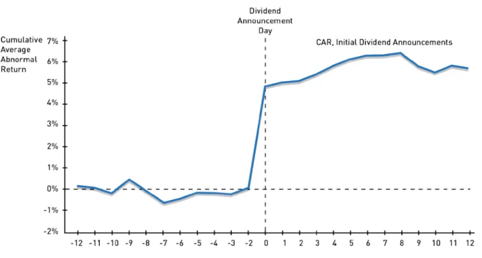
diagram. Here we reproduce the diagram from a study by Asquith and Mullins (1986) of the stock price reaction for 88 U.S. stocks around the time when the firms announced that they would start paying dividends. Time 0 marks the day the announcement of the dividend initiation was published in The Wall Street Journal, implying that the market learned the dividend news the day before, i.e., at time -1. The diagram plots the “cumulative abnormal returns,” i.e., the accumulated residual return 𝜀𝜀𝑡𝑡𝑖𝑖 from 12 trading days before until 12 trading days after the publication of the announcement. As seen in the diagram, dividend news is quickly incorporated in stock prices, with a large stock price reaction of about 5% around the announcement day, and insignificant abnormal returns before or after the announcement. This pattern indicates that this type of news has no predictability.
Figure 1: Abnormal stock returns for initial dividend announcements
The event-study methodology may seem simple, but the force of the original study by Fama, Fisher, Jensen and Roll and its results created a whole new subfield within empirical finance. An event study arguably offers the cleanest way of testing for whether new information is incorporated fully in prices, without generating predictable price movements. By and large, the vast majority of event studies have supported this hypothesis. Some exceptions have been found, however. The most notable and pervasive one probably is the so-called post-earnings announcement drift, first documented by Ball and Brown (1968).
One of the most common uses of event studies is to measure the value consequences of various events. If the market correctly incorporates the new information, the value effects of a particular event, such as a corporate decision, a macroeconomic announcement or a regulatory change, can be measured by averaging the abnormal returns across a large number of such events for different assets and time periods. This method has become commonly used to test predictions from various economic theories, in particular in corporate finance. See MacKinlay (1997) and Kothari and Warner (2007) for reviews of this extensive literature.
3.3 Subsequent studies of short-term predictability
A flood of empirical studies using longer time series and more refined econometric methods followed in the footsteps of the early work on predictability by Fama and others. Researchers found statistically significant short-term predictability in stock returns, but that such predictability is small in magnitude (e.g., French and Roll, 1986, Lo and MacKinlay, 1988, Conrad and Kaul, 1988). The autocorrelation turns out to be stronger for smaller and less frequently traded stocks, indicating that exploiting this predictability is very difficult, given trading costs. Focusing on the very short horizon, French and Roll (1986) compare the variance of per-hour returns between times when the market is open and weekends and nights when the market is closed. It turns out that prices vary significantly more when the market is open than they do over nights or weekends, measuring the price evolution per hour from closing to opening. This finding is intriguing, unless the intensity of the news is correspondingly much higher when the market is open. One interpretation is that uninformed “noise trading” causes short-term deviations of price from its fundamental value. Consistent with this, French and Roll found that higher-order autocorrelations of daily returns on individual stocks are negative. Although the interpretation of these findings is still subject to debate, a common explanation is that some of this predictability is due to liquidity effects, where the execution of large trades leads to short-term price pressure and subsequent reversals (Lehmann, 1990).
The research program outlined by Fama in his 1970 paper has by now yielded systematic evidence that returns on exchange-traded stocks are somewhat predictable over short horizons, but that the degree of predictability is so low that hardly any unexploited trading profits remain, once transaction costs are taken into account. In this specific sense, stock markets appear to be close to the no-arbitrage model with unpredictable forecasting errors. Lack of short-term predictability does not, however, preclude that longer-term stock market
returns could display considerable predictability. Even if short-term returns are nearly unpredictable, returns could quite possibly be predictable over longer time horizons. In the next section we turn to the evidence on longer-term predictability.
4.
Longer-term predictability
Studies of longer-term predictability have to confront the joint-hypothesis problem head on. To the extent that one is willing to maintain the hypothesis of arbitrage-free pricing, long-term return predictability would allow inference about the correct asset-pricing model. Conversely, finding long-term predictability may suggest the existence of arbitrage opportunities given a particular asset-pricing model.
Longer-term predictability of asset returns became a major research issue in the 1980s. The seminal contributions are attributable to Shiller. Important early contributions were also made by Fama; for example, Fama and Schwert (1977) showed that the short-term interest rate could be used to forecast the return on the stock market.
4.1Variance ratio tests
Are expected market returns constant over time or do they vary in a predictable way? Shiller addressed this question for bond markets (1979), as well as for stock markets (1981). He realized that the simple no-arbitrage hypothesis, with a constant expected return, could be tested by comparing the variance of asset returns in the short term and the long term. Until the early 1980s, most financial economists believed that cash-flow news was the most important factor driving stock market fluctuations. In the title of his 1981 paper, Shiller challenged this view by asking, “Do stock prices move too much to be justified by subsequent changes in dividends?”
To understand Shiller’s insight, recall that the basic pricing equation (1) implies that an asset price in an arbitrage-free market can be written as an expected present value of future “fundamentals”: the discounted value of future cash flows (dividends in the case of stocks), where discounting is represented by future values of 𝑚𝑚. As pointed out above, dividends as well as the discount factor are stochastic. Let 𝑃𝑃𝑖𝑖∗,𝑡𝑡 denote the realization of the fundamental value of a stock 𝑖𝑖 at time 𝑡𝑡, i.e., the discounted sum of future realized dividends from time t+1
unexpected movement in stock prices must come from a surprise change to 𝑃𝑃𝑖𝑖∗,𝑡𝑡, either due to a dividend movement or a movement in the stochastic discount factor. The theory thus says that 𝑃𝑃𝑖𝑖,𝑡𝑡 = 𝐸𝐸𝑡𝑡[𝑃𝑃𝑖𝑖∗,𝑡𝑡], so that the forecast error, 𝑃𝑃𝑖𝑖,𝑡𝑡− 𝑃𝑃𝑖𝑖∗,𝑡𝑡, must be uncorrelated with any information available today, in particular the current price. Otherwise the expectations would not make rational use of the available information. Because by definition 𝑃𝑃𝑖𝑖∗,𝑡𝑡 ≡ 𝑃𝑃𝑖𝑖,𝑡𝑡+
�𝑃𝑃𝑖𝑖∗,𝑡𝑡− 𝑃𝑃𝑖𝑖,𝑡𝑡� and the price and the forecast error are uncorrelated, it follows that 𝑉𝑉𝑣𝑣𝑟𝑟(𝑃𝑃𝑖𝑖∗,𝑡𝑡) =
𝑉𝑉𝑣𝑣𝑟𝑟(𝑃𝑃𝑖𝑖,𝑡𝑡) +𝑉𝑉𝑣𝑣𝑟𝑟�𝑃𝑃𝑖𝑖∗,𝑡𝑡− 𝑃𝑃𝑖𝑖,𝑡𝑡�, i.e., the variance of the realized fundamental value 𝑃𝑃∗ in a no-arbitrage market equals the sum of the variance of the price P and the variance of the forecast error. This implies that 𝑉𝑉𝑣𝑣𝑟𝑟�𝑃𝑃𝑖𝑖∗,𝑡𝑡�> 𝑉𝑉𝑣𝑣𝑟𝑟�𝑃𝑃𝑖𝑖,𝑡𝑡�. In other words, the variance of the price must be smaller than the variance of the realized discounted value of future dividends.
To investigate this relation empirically, Shiller (1981a) assumed a constant discount factor, which implies that (realized) fundamentals are given by
𝑃𝑃𝑖𝑖∗,𝑡𝑡 = � 𝑚𝑚𝑗𝑗 ∞ 𝑗𝑗=1
𝑑𝑑𝑖𝑖,𝑡𝑡+𝑗𝑗.
The resulting time series, based on dividends in the New York Stock Exchange, is displayed in the figure below together with the stock index itself. The contrast in volatility between the two series is striking. Contrary to the implication of the present-value model with constant discount rates, the price variance is much larger than the variance of the discounted sum of future dividends.8
The early excess-volatility findings were challenged on econometric grounds by Marsh and Merton (1986) and Kleidon (1986), who noted that the test statistics used by Shiller (1979, 1981) are only valid if the time series are stationary. This issue was addressed by Campbell and Shiller (1987). They used the theory of cointegrated processes, which had been recently developed by the 2003 Laureates Clive Granger and Robert Engle9, to design new tests of the
present-value model that allow the processes generating prices and dividends to be nonstationary. The model was again rejected, even under these more general and realistic conditions. The paper by Campbell and Shiller (1987) also was important in showing how
8At about the same time, and independently, LeRoy and Porter (1981) also studied the excess volatility of stock prices using a different methodology, where they constructed a joint test of price volatility and payoff volatility from a bivariate model for dividends and prices. They found evidence of excess volatility, but it appeared to be of borderline statistical significance.
9 See Engle and Granger (1987).
cointegration methods can be used as a natural extension of Fama’s (1970) notion of “weak form” tests.10
Figure 2: Real Standard and Poor’s Composite Stock Price Index (solid line p) and ex post rational price (dotted line p*), 1871–1979, both detrended by dividing a long-run exponential growth factor. The variable p* is the present value of actual subsequent real detrended dividends, subject to an assumption about the present value in 1979 of dividends thereafter.
4.2 Predictability in stock returns
The finding that stock and bond returns are more volatile in the short term than in the long term implies that returns are “mean reverting,” i.e., above-average returns tend to be followed by below-average returns and vice versa. This also implies that future returns can be predicted from past returns. Evidence that stock returns may be predictable in the medium and long term had started to emerge already in the 1970s. Basu (1977, 1983) documented that stocks with high earnings-to-price or dividend-to-price ratios outperform stocks with low ratios. Fama and Schwert’s (1977) investigation of the relationship between stock returns and inflation showed that periods of high short-term interest rates tend to be followed by lower subsequent stock-market returns.
10 Campbell and Shiller were also inspired by the work of Hansen and Sargent (1980), who showed how the concept
of Granger causality could be used in testing rational-expectation models.
The finding that stock prices are excessively volatile relative to dividends made it natural to focus on current dividend levels as a predictor of future returns. Shiller (1984) studied U.S. stock market data going back to the 1870s. By regressing the one-year-ahead rate of return on the current dividend-price ratio, he found a positive relationship: high dividends relative to price predict above-normal returns. Apparently, an investor could earn higher returns by going against the market, buying when prices are low relative to dividends and selling when prices are high. In a later paper, Campbell and Shiller (1988a) studied the predictive power of a long moving average of real earnings. They found that this variable has a strong power in predicting future dividends and that the ratio of this earnings variable to the current stock price is a powerful predictor of future stock returns. Other early studies of stock-return predictability include Keim and Stambaugh (1986) and Campbell (1987). These and other studies identified a variety of variables that forecast future stock returns. Typically these variables are correlated with key macroeconomic indicators, suggesting that the discount factor varies with the state of the business cycle.
Consistent with the limited predictability over very short horizons discussed in section 3, Fama and French (1988a) documented that predictability increases with the horizon. This finding is illustrated in the table below, taken from Cochrane (2001). Over a one-year horizon, the dividend/price ratio explains 15% of the variation in excess returns, but over a five-year horizon, the explanatory power is as high as 60%.11
Coefficients from regressing excess returns over different horizons on the ratio of dividend to price
Horizon (years) Coefficient (standard error) R2 1 5.3 (2.0) 0.15 2 10 (3.1) 0.23 3 15 (4.0) 0.37 5 33 (5.8) 0.60
11These regressions are associated with some econometric problems. The dividend-yield series is very persistent, and return shocks are negatively correlated with dividend-yield shocks. As a result, the return-forecast regression inherits the near-unit-root properties of the dividend yield. For such time series, standard test statistics may suffer from small sample biases. Nelson and Kim (1993) and Stambaugh (1999) have proposed methods for dealing with this problem. See also Cochrane (2007).
In a related contribution, Campbell and Shiller (1988b) explore the determinants of the dividend-price ratio, 𝑑𝑑𝑡𝑡⁄𝑃𝑃𝑡𝑡. Basic pricing theory implies that this ratio should reflect expectations of future dividend growth and discount rates. In the simplest case of no uncertainty, constant dividend growth at rate g, and a constant discount rate R, the pricing expression simplifies to 𝑑𝑑𝑡𝑡⁄𝑃𝑃𝑡𝑡 = 𝑅𝑅 − 𝑔𝑔, the so-called Gordon formula. In general, however, given its nonlinearity, implementing an asset-pricing equation for empirical studies is not straighforward. The methodology developed by Campbell and Shiller allows an analyst to gauge to what extent variations in d/P can be explained by variations in expected dividends and discount rates, respectively. It builds on a linearization that decomposes the logarithm of
d/P into a weighted sum of future expected log discount rates and log dividend changes. To generate expectations, Campbell and Shiller estimated a vector-autoregression system based on alternative measures of discount rates, e.g., interest rates and consumption growth. They found some evidence that d/P is positively affected by future dividend growth. None of the discount rate measures used, however, helped to explain the dividend-price ratio, and overall, most of the variation in this ratio remained unexplained. The Campbell-Shiller decomposition has become very influential both by providing an empirical challenge for understanding what drives asset prices and by providing a methodology for addressing this challenge.
4.3 Predictability in other asset markets
The findings of excess volatility and predictability by Shiller and others turned out to be a pervasive phenomenon, not only in the stock market but also in other asset markets. As a precursor to his work in 1980, Shiller (1979) already found evidence of excess volatility for government bonds. Under the assumption of a constant risk premium (the so-called expectations hypothesis), long-term interest rates should equal weighted averages of expected future short-term rates, and consequently the volatility of long-term rates should be smaller than the volatility of short-term rates. Shiller found just the opposite. The volatility of long-term rates turned out to be many times larger than the volatility of short-long-term rates. Similar to stock prices, the excess volatility of long-term bond prices implies that bond returns are predictable. Subsequently, Shiller, Campbell and Schoenholtz (1983), Fama and Bliss (1987), and Campbell and Shiller (1991) all found that the slope of the U.S. Treasury yield curve predicts bond returns at all maturities. Moreover, Campbell (1987) and Fama and French
(1989) showed that the term structure of interest rates predict stock returns as well, and that excess returns on long-term bonds and stocks move together.
Similar results were found in foreign exchange markets. According to the expectations hypothesis, forward exchange rates should be equal to expected spot rates. The expectations hypothesis implies that the so-called carry trade, which involves borrowing in a low-interest currency and investing in a high-interest currency, should not yield positive excess returns, as the higher interest rate should be offset by currency depreciation. Hansen and Hodrick (1980) developed econometric tests using multiple forward rates of different maturities, and were able to reject the expectations hypothesis in foreign exchange markets.12 Similarly, Fama
(1984) showed that the coefficient of the forward rate in a regression on future spot rates is actually negative, rather than plus one as the expectations hypothesis would predict. These studies, as well as many others that followed, indicated that foreign exchange markets exhibit significant return predictability as well.
The upshot from these results is that the volatility and predictability of stock, bond and foreign exchange returns can only be consistent with arbitrage-free markets if the expected return, i.e., the discount factor, is highly variable over time. The question then is whether theoretical models are able to generate such high variability in the discount factor.
5.
Risk premia and volatility in rational-agent models
The findings of excess volatility and predictability – and related findings, such as high return premia on stocks – by Shiller and other researchers illustrate the need for a deeper understanding of what drives the variation in expected returns over time. A major line of research, initiated in the 1970s, continues to strive to construct dynamic asset-pricing models that build on optimizing behavior, implying arbitrage-free prices. In a dynamic model, risk preferences of investors can vary over time, e.g., as a result of consumption or wealth shocks, thus generating fluctuations in risk premia and predictability of returns.
12The econometric approach taken by Hansen and Hodrick (1980) can be viewed as a precursor to Hansen’s (1982) GMM, discussed in section 5.3 below.
5.1 The consumption capital-asset–pricing model (CCAPM)
The most basic dynamic pricing model, the CCAPM, starts from the assumption that the economy can be described by a representative agent who maximizes expected utility given by
𝐸𝐸�∑ 𝛽𝛽𝑗𝑗𝑢𝑢(𝑐𝑐 𝑡𝑡+𝑗𝑗 ∞
𝑗𝑗=0 )|𝐼𝐼𝑡𝑡�,
where u is a utility function of consumption c and β is the subjective discount factor. Here, we write the conditional expectation 𝐸𝐸𝑡𝑡(∙) as 𝐸𝐸(∙|𝐼𝐼𝑡𝑡) in order to specify explicitly the information set 𝐼𝐼𝑡𝑡 on which the expectation is based. The agent faces a simple budget constraint
Σ𝑖𝑖𝑤𝑤𝑖𝑖,𝑡𝑡𝑃𝑃𝑖𝑖,𝑡𝑡+𝑐𝑐𝑡𝑡 ≤ Σ𝑖𝑖𝑤𝑤𝑖𝑖,𝑡𝑡−1(𝑃𝑃𝑖𝑖,𝑡𝑡+𝑑𝑑𝑖𝑖,𝑡𝑡) +𝑦𝑦𝑡𝑡,
where 𝑤𝑤𝑖𝑖,𝑡𝑡 is the number of units invested in the risky asset i at time t, 𝑑𝑑𝑖𝑖,𝑡𝑡 is the dividend generated by that asset, and 𝑦𝑦𝑡𝑡 is labor income at time t. The key equation of CCAPM is the first-order condition for utility maximum:
𝑢𝑢′(𝑐𝑐𝑡𝑡) =𝛽𝛽𝐸𝐸 �𝑢𝑢′(𝑐𝑐𝑡𝑡+1)∙𝑥𝑥𝑖𝑖,𝑡𝑡+1
𝑃𝑃𝑖𝑖,𝑡𝑡 |𝐼𝐼𝑡𝑡�.
Here, as before, 𝑥𝑥𝑖𝑖,𝑡𝑡+1 ≡ 𝑃𝑃𝑖𝑖,𝑡𝑡+1+𝑑𝑑𝑖𝑖,𝑡𝑡+1 is the asset’s payment at time t + 1. An optimizing agent is indifferent between consuming a unit at time t, thus receiving the marginal utility of one unit at that time (the left-hand side), and investing it to earn a rate of return 𝑥𝑥𝑡𝑡+1/𝑃𝑃𝑡𝑡 and obtaining the discounted marginal utility from consuming that at t + 1 (the right-hand side). This so-called Euler equation can be rewritten as an asset-pricing equation:
𝑃𝑃𝑖𝑖,𝑡𝑡= 𝐸𝐸 �𝛽𝛽𝑢𝑢
′(𝑐𝑐𝑡𝑡+1)
𝑢𝑢′(𝑐𝑐𝑡𝑡) ∙ 𝑥𝑥𝑖𝑖,𝑡𝑡+1|𝐼𝐼𝑡𝑡�. (2)
Equation (2) is thus a present-value equation of the same type as the one derived from the absence of arbitrage, equation (1), with the stochastic discount factor 𝑚𝑚𝑡𝑡+1 now given by
𝛽𝛽𝑢𝑢′(𝑐𝑐𝑡𝑡+1)/𝑢𝑢′(𝑐𝑐𝑡𝑡), which is the marginal rate of substitution between consumption today and tomorrow. This equation shows why the discount rate would be low during recessions: in bad times, when 𝑐𝑐𝑡𝑡 is low, the marginal utility 𝑢𝑢′(𝑐𝑐𝑡𝑡) is high, and thus the ratio of marginal utilities 𝑢𝑢′(𝑐𝑐𝑡𝑡+1)/𝑢𝑢′(𝑐𝑐𝑡𝑡) is correspondingly low (conversely, the discount factor should be high during booms).
The CCAPM would thus seem to give a possible qualitative explanation for the findings of predictability and excess volatility based on rational behavior. What about the quantitative content of the theory?
5.2 Testing the consumption capital-asset–pricing model (CCAPM)
Confronting economic theory with data is a methodological challenge, especially when the theory gives rise to nonlinear dynamic equations. For that reason, researchers often evaluate models informally, for example, by using calibration, where model parameters are selected based on non-statistical criteria and the model is solved and simulated. By comparing the resulting model-generated time series to actual data, calibration can be useful in assessing whether a model may be capable of quantitatively matching the actual data at all. A more rigorous approach, of course, would be to use formal statistical methods. But before the 1980s, the methodological challenges were daunting, and not until Hansen’s development of the GMM did formal tests of the CCAPM become commonplace. Thus, empirical evaluation of the CCAPM began with informal methods.
…using calibration and informal statistics
Grossman and Shiller (1981) were the first to evaluate the CCAPM quantitatively. They assumed utility to be given by a power function (implying constant relative risk aversion). The discount factor 𝛽𝛽𝑢𝑢′(𝑐𝑐𝑡𝑡+1)/𝑢𝑢′(𝑐𝑐𝑡𝑡) can then be calculated from consumption data for any given value of relative risk aversion. Using U.S. consumption data, Grossman and Shiller found, however, that the observed stock-price volatility could only be consistent with CCAPM if the marginal utility of consumption was extremely sensitive to variations in consumption, i.e., if the representative consumer was extremely risk averse. This finding left excess volatility as a challenge for future asset-pricing research. Subsequently, Shiller (1982) showed that the model implied a lower bound on the marginal rate of intertemporal substitution. This insight is a precursor to the influential contribution by Hansen and Jagannathan (1991), which is further discussed in Section 5.3.
In passing, Grossman and Shiller also noted that the CCAPM implied a much lower level of equity returns than observed in data, hence providing an early illustration of what Mehra and Prescott (1985) subsequently came to term the equity-premium puzzle. In their paper, Mehra and Prescott highlighted the extreme difficulty that traditional models have in matching an observed excess return of stocks relative to a risk-free asset of over 5% per year, a magnitude that had been observed in data for the U.S. and many other countries. To match the data, coefficients of relative risk aversion of around 50 were needed, and such levels of risk
aversion were viewed to be unrealistic from an applied microeconomic perspective, at least for the average investor.
… and using formal statistical methods
As discussed above, the CCAPM implies that returns are predictable as long as agents are risk averse and variations in consumption can be predicted. However, in order to test this theory researchers face several difficulties. One difficulty is the inherent nonlinearity of the main estimating equation. Another is the need to specify a full stochastic process for consumption. In fact, these difficulties, along with serial correlation of any errors in the dynamic system, are shared by a large set of models used in economics. In the early 1980s, the only way to handle these difficulties was by making a range of very specific assumptions – assumptions that were not even perceived to be central to the main issue at hand. Thus, any statistical rejection would be a rejection of the joint hypothesis of the main asset-pricing equation and all the specific assumptions to which the researcher was not necessarily wed.
An influential illustration of this point was given by Hansen and Singleton (1983), who dealt with the difficulties by a combination of approximations and specific assumptions. Assuming jointly normally distributed error terms, they developed the following log-linear version of CCAPM:
𝐸𝐸𝑡𝑡�ln�1 +𝑅𝑅𝑖𝑖,𝑡𝑡+1��=−ln𝛽𝛽 − 𝛾𝛾𝐸𝐸𝑡𝑡[Δln ct+1] + [𝜎𝜎𝑖𝑖 +𝛾𝛾2𝜎𝜎𝑐𝑐−2𝛾𝛾𝜎𝜎𝑖𝑖𝑐𝑐]/2.
This equation expresses expected log returns as the sum of three terms: the log rate of time preference β, a term that is multiplicative in the rate of risk aversion γ and the expected rate of consumption change, and a term that depends on variances and covariances. Hansen and Singleton then estimated this linearized model for monthly stock returns, using a maximum-likelihood estimator. Based on a value-weighted stock index, the model worked relatively well, giving estimates of relative risk aversion between zero and two and showing little evidence against the parameter restrictions. When estimated based on returns of individual stocks and bonds, however, the model was strongly rejected. This failure is an early indication of a serious challenge to the rational-agent–based asset-pricing model. At the time, however, it was unclear how much of the rejection was due to the linearization and error process assumptions and how much was an inherent limitation of the theory. The GMM provided a way to address these problems.
5.3 The Generalized Method of Moments (GMM) The asset-pricing context
Consider again the main equation of the CCAPM model, equation (2). Defining 𝑅𝑅𝑖𝑖,𝑡𝑡+1≡
𝑥𝑥𝑖𝑖,𝑡𝑡+1/𝑃𝑃𝑖𝑖𝑡𝑡, it can be rewritten as 1 = 𝐸𝐸 �𝛽𝛽𝑢𝑢′(𝑐𝑐𝑡𝑡+1)
𝑢𝑢′(𝑐𝑐𝑡𝑡) ∙𝑅𝑅𝑖𝑖,𝑡𝑡+1|𝐼𝐼𝑡𝑡�. (3)
This is a nonlinear function of the stochastic processes for consumption and returns and any relevant additional variables in the conditioning set 𝐼𝐼𝑡𝑡. The expression 𝛽𝛽𝑢𝑢′(𝑐𝑐𝑡𝑡+1)
𝑢𝑢′(𝑐𝑐𝑡𝑡) ∙𝑅𝑅𝑖𝑖,𝑡𝑡+1−1 can
be regarded as a one-period-ahead forecast error. Under rational expectations, this error must be independent of any information It available at time t. Let us use zjt to denote a variable in
the information set It, e.g., a historical asset price. This implies, for any asset i and
conditioning variable or “instrument” zj, that 𝐸𝐸 ��𝛽𝛽𝑢𝑢′(𝑐𝑐𝑡𝑡+1)
𝑢𝑢′(𝑐𝑐𝑡𝑡) ∙𝑅𝑅𝑖𝑖,𝑡𝑡+1−1� ∙ 𝑧𝑧𝑗𝑗𝑡𝑡|𝐼𝐼𝑡𝑡�= 0. (4)
This equation, which is an implication of equation (3), is the basis for GMM estimation of an asset-pricing model.
Some econometric theory
Equation (4) can be viewed as an element in the following vector equation
𝐸𝐸𝒈𝒈(𝒙𝒙𝑡𝑡,𝜽𝜽) =𝟎𝟎 (5)
where 𝒙𝒙𝑡𝑡 is a vector stochastic process (sequence of random variables) and 𝜽𝜽 is a parameter vector to be estimated. The vector-valued function 𝒈𝒈 expresses the key orthogonality condition – one equation for each asset i and instrument 𝑧𝑧𝑗𝑗𝑡𝑡. In the example, 𝒙𝒙𝑡𝑡 consists of 𝑐𝑐,
𝑅𝑅𝑖𝑖 (for all assets 𝑖𝑖), and 𝑧𝑧𝑗𝑗𝑡𝑡 (for at least one instrument j), and 𝜽𝜽 consists of 𝛽𝛽 and the other parameters in (4). The (i,j)th element of the 𝒈𝒈 vector would thus be�𝛽𝛽𝑢𝑢′(𝑐𝑐𝑡𝑡+1)
𝑢𝑢′(𝑐𝑐𝑡𝑡) ∙𝑅𝑅𝑖𝑖,𝑡𝑡+1−1� ∙ 𝑧𝑧𝑗𝑗𝑡𝑡,
for asset 𝑖𝑖 and a particular instrument 𝑧𝑧𝑗𝑗𝑡𝑡. This element has expectation zero and can be interpreted as a form of forecast error.
In a paper that has turned out to be one of the most influential papers in econometrics, Hansen (1982) suggested the GMM as an attractive approach for estimating nonlinear systems like equation (5). A main reason why this estimator has become so popular is that it places only
very weak restrictions on the stochastic process 𝒙𝒙𝑡𝑡, which is allowed to be any weakly stationary, ergodic process, and on 𝒈𝒈, which is allowed to be nonlinear. This generality is particularly important in panel-data and time-series applications, such as asset pricing ones, where the stochastic process is correlated and the key relationships are nonlinear. Moment conditions such as (5) had been used in parameter estimation since Pearson (1894, 1900), see also Neyman and Pearson (1928), but their use had been confined to cases where the components of 𝒙𝒙𝑡𝑡 are independent over time, e.g., as in the case of repeated independent experiments. Hansen’s contribution was to generalize the previous theory of moment estimation to the case where 𝒙𝒙𝑡𝑡 is a stationary and ergodic process.
The GMM estimator can be defined using the sample moment function
𝒈𝒈𝑇𝑇(𝜽𝜽) ≡1𝑇𝑇� 𝒈𝒈(𝒙𝒙𝑡𝑡,𝜽𝜽) 𝑇𝑇
𝑡𝑡=1 and the quadratic form
𝑆𝑆𝑇𝑇(𝜽𝜽)≡ 𝑇𝑇𝒈𝒈𝑇𝑇(𝜽𝜽)′𝑾𝑾𝒈𝒈𝑇𝑇(𝜽𝜽),
where 𝑾𝑾 is a positive definite weight matrix. The GMM estimator 𝜽𝜽�𝑇𝑇 minimizes 𝑆𝑆𝑇𝑇(𝜽𝜽). Hansen (1982) showed that this estimator is consistent for the true parameter vector under certain regularity conditions and that it is asymptotically normal given some mild restrictions on 𝒈𝒈(𝒙𝒙𝑡𝑡,𝜽𝜽). As already indicated, the proof allows rather general stochastic temporal dependence for the stochastic process 𝒙𝒙𝑡𝑡.
Furthermore, Hansen defined the asymptotic covariance matrix
𝜴𝜴 ≡ ∑∞𝒋𝒋=−∞𝐸𝐸𝒈𝒈𝑡𝑡(𝜽𝜽)𝒈𝒈𝑡𝑡−𝑗𝑗(𝜽𝜽)′.
Hansen showed that the selection 𝑾𝑾=𝜴𝜴−1 ensures that the resulting estimator 𝜽𝜽�𝑇𝑇 minimizes (in the matrix sense) the asymptotic covariance matrix of the estimator. This result provides an asymptotic efficiency bound for the GMM estimator – a bound because the true 𝞨𝞨 is not known.
Hansen also showed how to estimate the asymptotic covariance matrix and, using its inverse as a weighting matrix, derived the resulting asymptotic normal distribution. Hansen’s construction of the estimate of 𝜴𝜴 is based on a consistent estimate of 𝜽𝜽for the sample at hand, but at the same time, the estimated 𝜴𝜴 is needed to construct an efficient estimate of 𝜽𝜽 This conundrum means that there is no straightforward way of obtaining the efficient estimate. Hansen therefore proposed a two-stage procedure: start with an arbitrary weighting matrix
and use it to construct a consistent estimator and use that estimator to estimate the asymptotic covariance matrix; then use that matrix to obtain the efficient estimator of 𝜽𝜽. Alternative procedures were proposed later to improve on this two-stage approach.
Finally, Hansen demonstrated how to construct a test of over-identifying restrictions, based on a method proposed by Sargan (1958). Under the null hypothesis this test statistic has an asymptotic 𝜒𝜒2 distribution with 𝑘𝑘 − 𝑟𝑟 degrees of freedom, where 𝑘𝑘 is the number of moment conditions and 𝑟𝑟 the number of linear combinations of these conditions (to find 𝑟𝑟 parameters of interest).13
In summary, Hansen provided the necessary statistical tools for dealing with estimating dynamic economic models using panel data, where serially correlated variables are commonplace and where specifying a full model is not always desirable or even possible; GMM can be applied to a subset of the model equations. GMM has made a huge impact in many fields of economics where dynamic panel data are used, e.g., to study consumption, labor supply or firm pricing. It is now one of the most commonly used tools in econometrics, both for structural estimation and forecasting and in microeconomic as well as macroeconomic applications.14
The asset-pricing application
Equipped with GMM, researchers analyzing asset prices could now go to work. The first direct application of Hansen’s GMM procedure is reported in the paper on asset-pricing by Hansen and Singleton (1982). But an earlier use of the essential idea behind GMM can be found in work by Hansen and Hodrick (1980), who looked at currencies and asked whether forward exchange rates are unbiased predictors of future spot rates. Serial correlation in errors and nonlinearities make traditional approaches invalid for this issue, and the authors derived asymptotic properties based on methods that turned out to be a special case of GMM.
The main purpose of Hansen and Singleton (1982) was to test the CCAPM. To operationalize the model, the authors assumed utility, as did Grossman and Shiller (1981), to display
13Hansen has followed up his seminal piece with a number of important extensions, including alternative estimators (Hansen, Heaton and Yaron, 1996), the choice of instruments (Hansen, 1985, and Hansen, Heaton and Ogaki, 1988), continuous-time models (Hansen and Scheinkman, 1995), and GMM with non-optimal weighting matrices (Hansen and Jagannathan, 1997).
14See the review articles by Hansen and West (2002) and Jagannathan, Skoulakis and Wang (2002) for illustrations of the use of GMM in macroeconomics and finance. In microeconometrics, GMM has also been a commonly used model for estimation with panel data – see Arellano and Bond (1991) and Blundell and Bond (1998).