Modified Discrete Binary PSO based Sensor Placement for Coverage in WSN Networks

Modified Discrete Binary PSO based Sensor

Placement for Coverage in WSN Networks

Neha Jain 1, Kanchan Sharma 2

Department of Electronics and Communication Indira Gandhi Institute of Technology, Delhi

1_{[email protected],} 2_{[email protected]}

Abstract- The main idea of this paper is to solve coverage problem in distributed wireless sensor network (WSN) by increasing sensor nodes coverage. This paper proposes a modified discrete binary particle swarm optimization algorithm for Wireless Sensor Network (WSN) nodes placement so that the maximum coverage is obtained.PSO is a real value algorithm, and the discrete PSO is proposed to be adapted to discrete binary space. The proposed algorithms are going to solve the problem by considering the factor on the sensor deployment scheme, given a finite number of sensors, optimizing the sensor deployment will provide sufficient sensor coverage. The proposed method on sensors surrounding is examined in different area. The results not only confirmed the successes of using new method in sensor replacement, but also they showed that the new method performs more efficiently.

Keywords— Modified Discrete Binary PSO, Distributed Sensor Placement, Coverage, Sensor Placement

I. INTRODUCTION

A wireless sensor network (WSN) is one of the communication networks that have been used nowadays. A typical wireless sensor network consists of thousands of sensor nodes, deployed either randomly or according to some predefined statistical distribution, over a geographic region of interest. Spatially distributed sensors are employed in WSN to monitor environmental or physical conditions, vibration, pressure, motion, temperature and pollutant. The range of potential applications that WSNs are envisaged to support, is tremendous .Some WSN application area military applications like communication systems, commanding, reconnaissance patrols, looking –out etc, environmental and natural resource monitoring , medical, industrial, robot, air forecasting, security, anti terrorism applications and civilian applications. Cost and size constraints on sensor nodes yield subsequent constraints on resources such as bandwidth, energy, computational speed and memory .These limitations have given many technical problems such as routing, scheduling and coverage and cost. Distributed sensor network can arrange in two ways, one as a random placement and the second as a grid-based placement. When the surrounding is unknown the random placement is used but when the properties of the network were known before then the sensor placement could be done with great investigation so that we could guarantee the quality of services. The strategy of sensor placement depends on the application of the distributed sensor network (DNS). In this paper we focus on the gird-based placement. The sensor network which is based on grid-based plcement is considered as a two or three dimensional network. And we applied the modified binary PSO algorithm for solve the problems like coverage and cost.

II.PSO:ABRIEF OVERVIEW

PSO is a population-based optimization algorithm, inspired by the social behaviour of flocks of birds or fishes. Each particle is an individual and the swarm is composed of particles. The problem solution space is formulated as a search space. Each position in the search space is a correlated solution of the problem. In a PSO system, each particle is “flown” through the multidimensional search space, adjusting its position in search space according to its own experience and that of neighboring particles.

Suppose a group of birds are searching for food in a place randomly and food is available in one part of searching area and the birds have no information about the place where the food is available and they only know their distance to the food source. The adopted strategy by birds is that they follow the bird which has minimum distance to the food source. In PSO algorithm, each answer to the problem is considered as a bird in the search space which is called a particle. Each particle has its own fitness determined by the fitness function. A bird which is close to food source has a better fitness.

There are many subjects which have discrete nature and because there are many problems which have a discrete nature and also because many of both discrete and continuous problems can be solved in a discrete space so there is a need to use the binary PSO algorithm.

The features of the method are as follows:

(1) The method is based on researches on swarms such as fish schooling and bird flocking.

(2) It is based on a simple concept. Therefore, the computation time is short and it requires few memories [4].

A. The PSO Algorithm

PSO is developed through simulation of bird flocking in two-dimension space. The position of each individual particle is represented by XY axis position and also the velocity is expressed by VX (the velocity of X axis) and Vy (the velocity of Y

axis). Modification of the particle position is realized by the velocity and position information. Each particle knows its best value pbest and its XY position. Moreover, each particle knows the best value in the group gbest among pbest. Each particle tries to change its position using the following information [4]:

a) The current velocities (Vx, Vy),

b) The distance between the current position, and pbest and gbest. c) The current positions (x, y)

This change can be represented by the concept of velocity and of each particle can be changed by the following equation:

st-Xi (t)) (1) The current position (searching point in the solution space) can be modified by the following equation:

Xi (t+1) = Xi (t) +Vi (t+1) (2) where, Vi (t) Velocity of agent, c1 & c2 are weighting factor, w is weighting function, rand( ) is random function, Xi (t) is

current position of particle, pibest is best of particle and gbest is best of the group. III. COVERAGE IN WSN

Sensor’s prime function is to sense the environment for any occurrence of the event. Thus, coverage is one of the major concerns in WSN. It becomes a key to calculate the quality of service (QoS) in WSN [3]. There are three main reasons that cause coverage problem in WSN. They are limited sensing range, random deployment, and not enough sensors to cover the whole ROI. The limited power supply effects the sensor’s operation. It will reduce the coverage rate and result in inadequate sensors to cover the whole ROI as some them might die out. Choosing a sensor with larger sensing can resolved the limited sensing range problem but the price of it will be more expensive. One of the problems arises when some of the sensors are deployed too far apart while the others are too close to each other in random deployment. Therefore, to remove these coverage problems, we need to focus on the problem during deployment phase or predetermine the deployment of sensors. In predetermine deployment the coverage becomes better by caution planning of the positions of the sensors in the ROI.

Three types of coverage have been defined:

• Area Coverage: It suggests how to cover an area which maximizes the detection rate of targets appearing in the sensing field.

• Barrier coverage: To achieve a static arrangement of sensor nodes, this minimizes the probability of undetected penetration through the barrier.

• Point coverage: It deals with coverage for a set of points point interest.

The strategies used in solving coverage problem in WSN which are done during deployment stage are divided into three categories force based, grid based and computational geometry based.

Force Based: It uses virtual repulsive and attractive forces. The sensors are force to move away or towards each other so that full coverage is achieved. Force based deployment strategies rely on the sensor’s mobility The sensors will keep

moving until equilibrium state is achieved where repulsive and attractive forces are equal thus they end up cancelling each other.

Grid Based: Grid points are used in two ways in WSN deployment 1) To measure coverage

2) To determine sensors positions.

Coverage percentage is defined as ratio of area covered to the area of ROI. However to calculate the area of irregular shape due to overlapping of sensing range is a difficult task. Therefore researcher had used sampling methods. In sampling methods only a set of points inside the ROI is used to evaluate the coverage. The coverage is calculated as ratio of grid points covered to total number of grid points in the ROI. The cost of grid based method calculated by number of grid points; n×m and amount of sensors deployed, k [9].

Computational geometry Based: This method is frequently used in WSN coverage optimization. The most commonly used computational geometry approaches are Voronoi diagram and Delaunay triangulation [10].

IV. MDPSO ALGORITHM

There are many subjects which refer to discrete nature. Many problems have discrete and both discrete and continuous nature. So there is need to use the binary PSO algorithm. PSO is initialized with a group of random particles (solutions) and then searches for optimal solutions by updating the position of particles. Each particle is distinguished by an Nd

dimensional vector (the number of points of sensor field) along with two values Xid (current position of particle)and Vid

(velocity of particle) where, Xid =( Xid1,…..Xidn) and Vid = (Vid1…..Vidn ),where i denotes the particle and d denotes the

dimension search space [3].

In binary PSO model, Vid defines the probability of value of one Xid .Position of each particle defines in region of one and

zero (0, 1) while Vid is defined as probability function so it is limited in the range of one and zero (0, 1). Therefore, the

particle position can be update by using equation (5). In this the new position component has to be exchanged with a value of probability obtained by applying modified sigmoid transformation to the velocity component (see equation (4)).The value of vid can be high, low or zero. If the value of Vid is high the particle’s position is unfit therefore it causes the value of

Xid to changed from 0 to 1 or vice versa. If the value of vid is low for Xid it decreases the probability of changes in the value

of Xid. And the value of Xid is unchanged if the value of vid is zero according to equation (5).

Velocity of each particle can be modified by the following equation:

Xid (t))

d = 1,2...Nd (3)

Where, c1 & c2 are weighting factor or learning coefficients. Usually c1 is equal to c2, and they are in the range (1, 2).w is

weighting function or inertia factor, usually is a number in the range (0, 1), rand ( ) is random function in the range of (0, 1), x (t) is current position of particle, pbest is best of particle and gbest is best of the group. The final value for velocity of each particle is limited to avoid the divergence: Vid Є [-vmax, vmax]. Typically, this process is iterated for a certain

number of time steps, or until some acceptable solution has been found by the algorithm. Sig (Vid) =1/ (1+e-vid)

S’(Vid) = 2˟ |Sig (Vid) -0.5| (4)

If rand < s’ (Vid (t+1) then

Xid (t+1) = exchange (Xid)

else Xid (t+1) = (Xid) (5)

Power Vector for each grid point formula is

pvi = (pv1, pv2, …………pvik)

pvi ={1, pvi is 1 if target location at I can be detected by the sensor at location k 0, otherwise

V.

S

MATLAB software is used to simulate the algorithm. In the simulation some basic parameters for PSO are: maximum iteration is 1000, maximum velocity is 6, inertia weight is 0.9-0.2, learning factors c1, and c2 are in the range (1, 2). From

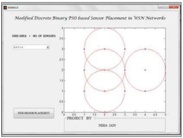
the simulation diagrams, the blue colour dots indicate grid points and red colour indicates sensor points. Sensor points are on grid points. The red dotted circles around each sensor points represent the coverage area. Fitness function is sum of ones in particle here, it indicate cost of sensors that used for coverage the field sensor completely. The different cases obtained from algorithm simulation are shown and discussed in this paper.

In case 1, the total numbers of grid points are 12 (4×3) which are shown by the blue dots. By the simulation algorithm, the number of sensors required to cover all the grid points are 4. These are shown by red points and the areas covered are shown by red circles Fig (1).

Fig 1 Case 1- Area of 12 covered by 4 sensors

In case 2, the total numbers of grid points are 18 (6×3) which are shown by the blue dots. By the simulation algorithm, the number of sensors required to cover all the grid points are 6. These are shown by red points and the areas covered by these sensors are shown by red circles Fig (2).

Fig 2 Case 2-Area of 18 covered by 6 sensors

In case 3, the total numbers of grid points are 24 (6×4) which are shown by the blue dots. By the simulation algorithm, the number of sensors required to cover all the grid points are 8. These are shown by red points and the areas covered by these sensors are shown by red circles Fig (3).

Fig 3 case 3- Area of 24 covered by 8 sensors

In case 4, the total numbers of grid points are 21 (7×3) which are shown by the blue dots. By the simulation algorithm, the number of sensors required to cover all the grid points are 7. These are shown by red points and the areas covered by these sensors are shown by red circles Fig (4).

Fig 4 Case 4- Area of 21 covered by 7 sensors

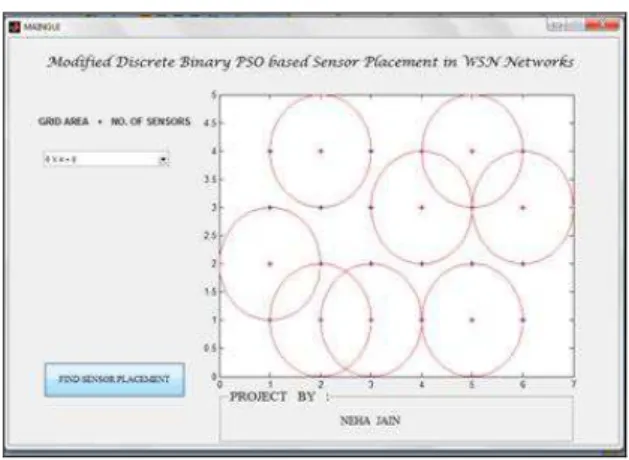
In case 5, the total numbers of grid points are 24 (8×3) which are shown by the blue dots. By the simulation algorithm, the number of sensors required to cover all the grid points are 9. These are shown by red points and the areas covered by these sensors are shown by red circles Fig (5).

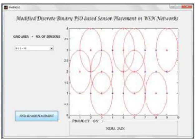
In case 6, the total numbers of grid points are 27 (9×3) which are shown by the blue dots. By the simulation algorithm, the number of sensors required to cover all the grid points are 10. These are shown by red points and the areas covered by these sensors are shown by red circles Fig (6).

Fig 6 Case 6- Area of 27 covered by 10 sensors

In case 7, the total numbers of grid points are 16 (4×4) which are shown by the blue dots. By the simulation algorithm, the number of sensors required to cover all the grid points are 4. These are shown by red points and the areas covered by these sensors are shown by red circles Fig (7).

Fig 7 Case 7 - Area of 16 covered by 4 sensors

All the cases are shown in the table given below.

TABLE 1

No. of Sensor Required as Per Area

Case Grid Area Sensors

1 4*3 4 2 6*3 6 3 6*4 8 4 7*3 7 5 8*3 9 6 9*3 10 7 4*4 4

VI. CONCLUSION

The sensor placement problem for locating targets under constraint (complete coverage of sensor networks) is considered in this paper. The problem with sensor network coverage is explained first and then the modified binary PSO algorithm is used to solve the problem. The results showed that the MDPSO algorithm is able to detect more effectively the optimization solution in a limited time, which provides placement of sensors to increase the coverage on the sensor field. In addition the proposed algorithm is more useful, scalable and durable.

VII.

R

[1] Shi Y.H. and Eberhart R.C. (1998) “A modified particle swarm optimizer,” IEEE International Conference on Evolutionary Computation, Anchorage, Alaska, pp.:69-73, May 4-9, 1998.

[2] Shirin Khezri , Karim Faez , Amjad Osmani , “Modified Discrete Binary PSO based Sensor Placement in WSN Networks,” Proceedings of the IEEE Computational Intelligence and Communication Networks (CICN), 2010 International Conference in Bhopal, pp.: 200 - 204 , Nov. 2010.

[3] Wan Ismail, W.Z., Manaf, S.A. , “Study on Coverage in Wireless Sensor Network using Grid Based Strategy and Particle Swarm Optimization,” in Circuits and Systems (APCCAS), IEEE Asia Pacific Conference, pp.:1175 – 1178, 2010.

[4] ZHANG Yuli, ZHU Xi, “Wireless Sensor Network Path Optimization Based on Particle Swarm Algorithm,” in Computer Science and Automation Engineering 2011 IEEE International Conference in vol. 3, p.p.: 534-537, 2011.

[5] Amjad Osmani, “Design and evaluation of two distributed methods for sensors placement in Wireless Sensor Networks,” in Journal of Advances in Computer Research, p.p.: 13-26, 2011.

[6] Y.Zou, K.Chakrabarty, “Sensor deployment and target localization in distributed Sensor networks,” Proceedings of the Trans .IEEE Embedded Comput .Syst. Vol 3, No.1, 2004.

[7] R. Rajagopalan, R. Niu, Ch. K. Mohan, P. K. Varshney, A.L. Drozd, “Sensor placement algorithms for target localization in sensor networks”, Proceedings of the IEEE Radar Conference, pp.: 1-6, 2008.

[8] Raghavendra V. Kulkarni, and Ganesh Kumar Venayagamoorthy, “Particle Swarm Optimization in Wireless Sensor Networks: A Brief Survey,” in Systems, Man, and Cybernetics, Part C: Applications and Reviews, IEEE Transactions, Volume: 41, Issue: 2, p.p.: 262-267, march 2011.

[9] Shen. X., Chen, J., Wang, Zhi. And Sun, Y. “Grid Scan: A Simple and Effective Approach for Coverage Issue in Wireless Sensor Networks,” IEEE International Communications Conference, Volume: 8, pp.: 3480-3484, June 2006.

[10] Nor Azlina Ab. Aziz, Kamarulzaman Ab. Aziz, and Wan Zakiah Wan Ismail “Coverage Strategies for Wireless Sensor Networks,” in World Academy of Science, Engineering and Technology 50, 2009.

[11] Mojtaba Ahmadieh Khanesar, Hassan Tavakoli, Mohammad Teshnehlab and Mahdi Aliyari Shoorehdeli, “Novel Binary Particle Swarm Optimization,” K N. Toosi University of Technology, Iran.

[12] Nor Azlina bt Ab Aziz, Ammar W. Mohemmed and Mohammad yusoff Alias, “A Wireless Sensor Network Coverage optimization Algorithm Based on Particle Swarm Optimization and Voronoi Diagram,” International Conference on Networking, Sensing and Control, ICNSC’09, pp.: 602-607, 2009.

[13] J. Kennedy and R. Eberhart, “Particle swarm optimization,” in proceedings of the IEEE International Conference on Neural Networks, vol. 4,pp. 1942-1948, 27 Nov., Dec. 1995.

[14] Dian Palupi Rini, Siti Mariyam Shamsuddin, Siti Sophiyati Yuhaniz, “Particle Swarm Optimization: Technique, System and Challenges,” in International Journal of Computer Application (0975-8887), Volume 14- No. 1, January 2011.