A general framework for functional regression
modelling
Sonja Greven1and Fabian Scheipl1
1Department of Statistics, Ludwig-Maximilians-Universit ¨at M ¨unchen, Germany
Abstract: Researchers are increasingly interested in regression models for functional data. This article discusses a comprehensive framework for additive (mixed) models for functional responses and/or functional covariates based on the guiding principle of reframing functional regression in terms of corresponding models for scalar data, allowing the adaptation of a large body of existing methods for these novel tasks. The framework encompasses many existing as well as new models. It includes regression for ‘generalized’ functional data, mean regression, quantile regression as well as generalized additive models for location, shape and scale (GAMLSS) for functional data. It admits many flexible linear, smooth or interaction terms of scalar and functional covariates as well as (functional) random effects and allows flexible choices of bases—particularly splines and functional principal components—and corresponding penalties for each term. It covers functional data observed on common (dense) or curve-specific (sparse) grids. Penalized-likelihood-based and gradient-boosting-based inference for these models are implemented in R packagesrefundandFDboost, respectively. We also discuss identifiability and computational complexity for the functional regression models covered. A running example on a longitudinal multiple sclerosis imaging study serves to illustrate the flexibility and utility of the proposed model class. Reproducible code for this case study is made available online.
Key words: functional additive mixed model, functional data, functional principal components, GAMLSS, gradient boosting, penalized splines
1 Introduction
1.1 Background and aims
Recent technological advances generate an increasing amount of functional data where each observation represents a curve or an image instead of a scalar or multivariate vector (Ramsay and Silverman, 2005; Horv ´ath and Kokoszka, 2012). Functional data occur in medicine and biology, economics, chemistry and engineering as well as phonetics but are certainly not limited to these areas. Examples of technologies that generate functional data include imaging techniques, accelerometers, spectroscopy and spectrometry as well as any kind of measurement collected over time, data usually referred to as longitudinal. The term ‘functional’ data Address for correspondence: Sonja Greven, Department of Statistics,
Ludwig-Maximilians-Universit ¨at M ¨unchen, Ludwigstr. 33, 80539 Munich, Germany. E-mail: [email protected]
traditionally refers to data measured over an interval in the real numbers, although it is broader in meaning, for example also referring to functions on higher dimensional domains such as images over domains T in R2 or R3 or functions over manifolds.
In this article, we will focus on functional data over a real intervalT, where curves could be observed on a dense grid common to all functions, with missings, or even on sparse irregular grids that are curve-specific. Sparse functional data commonly occur for longitudinal data that are viewed as functional data.
As functional data become more common, researchers are increasingly interested in relating functional variables to other variables of interest, that is in regression models for functional data. In addition, it becomes apparent that many complications well known from scalar data can and do also occur for functional data. Study designs or sampling strategies induce dependence structures between functions, for example, due to crossed designs, longitudinal or spatial settings. While more traditional functional data can be seen as realizations from stochastic processes that are often assumed to be Gaussian with some kind of smoothness assumption over the interval
T, there is a rising number of datasets where the observations consist of counts or binary quantities or follow skewed, bounded or otherwise non-normal distributions. It is thus also of interest to develop methods for ‘generalized’ functional data from non-Gaussian processes and/or to model other quantities of the conditional response distribution than (just) the mean.
In this article, we will focus on quite general, flexible models for regression with functional responses and/or covariates, with the aim of providing a similar amount of flexibility and modularity for functional data as the models that are presently available for scalar data—such as generalized additive mixed models (GAMMs), GAMLSS or (semi-parametric) quantile regression—and, in fact, strongly relying on recent advances in these areas. With this goal in mind, we will not provide a comprehensive review of available methods for functional regression(cf.Morris, 2015; Reiss et al., 2016; Wang et al., 2016), many of which are focused on one particular functional model at a time. We hope, instead, to provide a readable introduction to flexible functional regression within one overall consistent framework, also covering the implementation in R packagesrefund(Huang et al., 2016)andFDboost(Brockhaus and R ¨ugamer, 2016). While the general framework we introduce, the notation we use and the estimation approaches we describe are largely based on the work of our own group and of our collaborators over the last few years, many of the particular functional regression models discussed in the literature (Morris, 2015; Reiss et al., 2016; Wang et al., 2016)can be seen as special cases of this framework. We point out connections and different approaches to estimation along the way, while keeping the focus on a unified set-up. We believe that having such a unified framework facilitates discussion, implementation and practical use of flexible functional regression models. Connecting their estimation to corresponding approaches for scalar data as we do here additionally ensures that recent and future advances in inference for such scalar regression models can be immediately used to expand the model class or improve inference for all functional models covered by this general framework. We are necessarily taking a somewhat subjective view coloured by the type of functional data and algorithms that we have worked on. Note that other approaches might
be better suited to different kinds of functional data including spiky (e.g., Morris et al., 2006)or truly big functional data(e.g.,Zipunnikov et al., 2011; Reimherr and Nicolae, 2016).
1.2 Running example
As a running example, we will use a study on multiple sclerosis (MS) (Greven et al., 2010), which has been widely used as an example in the functional data literature. The dataset is available in the R package refund (Huang et al., 2016)
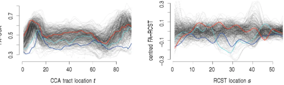
and we can thus make our analysis fully reproducible in the code supplement provided for this article. This study followed 100 MS patients and 42 healthy controls longitudinally over time. At each of their up to eight visits (median number of visits: 2), subjects underwent a Diffusion Tensor Imaging (DTI) scan of their brain. MS patients additionally completed a Paced Auditory Serial Addition Test (PASAT) measuring abilities relating to information processing and attention, resulting in a scalar score. Fractional anisotropy (FA), which is related to directedness of water diffusion, was then extracted from the DTI scans along two major tracts in the brain—the corpus callosum (CCA) and the right corticospinal tract (RCST). FA is used as a proxy of demyelination, which acts as a marker of disease progression in MS since MS damages the myelin coating of the axons in the brain and thus impacts information transmission. FA values were averaged over slices of each tract, resulting in a scalar summary along one dimension of the tract. The procedure thus results in two functional variables for the two tracts, defined as functions of spatial distance along the tract. Figure 1shows observed FA values for the two tracts we consider: The left panel shows CCA tracts, while the right panel shows centred and smoothed FA values along the RCST tracts. The coloured lines code for specific subjects (see the caption).
Figure 1 DTI data: Left panel shows observed FA values along the CCA tracts, right panel shows the centred and smoothed FA values along the RCST tracts. Blue and cyan lines show FA curves for selected MS patients with PASAT scores of 30 and 60, respectively. Red lines show curves for a control subject.
1.3 Functional regression models
The DTI data nicely illustrate that, depending on the question of interest, regression for functional data can occur in at least three flavours.
• If interest lies in quantifying the difference in FA–CCA profiles between cases and controls at the first visit, then we would use function-on-scalar regression(Reiss et al., 2010) for a functional response with a scalar covariate. A simple linear model would be
Yi(t)=ˇvi(t)+Ei(t)+εit, (1.1)
where Yi(t) is the FA–CCA profile for subject i at the first visit at distance
t along the tract, ˇvi(t) represents a group-specific functional intercept with
vi =1[0] denoting subjects i belonging to the MS patients [controls], Ei(t) a
smooth residual andεit additional white noise error.
• If we are interested in whether the FA along the CCA is predictive of the PASAT score measured at the first visit, then we have a scalar response and a functional covariate, that is, scalar-on-function regression also known as signal regression
(Marx and Eilers, 1999) or functional linear model (Cardot et al., 1999) if the effect is linear. In this case, a simple linear model for the first visits of the MS patients is
Yi =˛+
Sxi(s)ˇ(s)ds+εi, (1.2)
withYinow the PASAT score for subjectiandxi(s) denoting the FA–CCA profile
observed at tract location sin S,ˇ an unknown weight or coefficient function andεi independent and identically distributed (i.i.d.) errors.
• If the focus lies on the relationship between the FA profiles along the two tracts, then we could think of a regression model with a functional response and a functional covariate (e.g., Ramsay and Silverman, 2005, Chapter 12), that is, function-on-function regression. A linear regression model in this case could be
Yi(t)=˛(t)+
Sxi(s)ˇ(s, t)ds+Ei(t)+εit, (1.3)
with Yi(t) andxi(s) now referring to the CCA– and FA–RCST profiles observed
attin intervalTandsinSrespectively,ˇ(s, t) a bivariate coefficient quantifying the association between xat spatial locationswith Y at spatial locationt, and Ei(t) andεit as in model (1.1).
Several extensions could also be considered. Models (1.1)–(1.3) all assume linear relationships between responses and covariates, which we might want to relax to more general smooth association structures. Also, the DTI data were collected longitudinally, and if we want to consider all observations simultaneously instead
of only the first visit, then we need to take into account the resulting correlation structure. Random effects are commonly used for scalar longitudinal observations and could be included in model (1.2), but for functional responses, we need functional analogs of random effects. We might want to modify model (1.3), for example, to
Yaw(t)=˛(t)+
Sxaw(s)ˇ(s, t)ds+Ba(t)+εawt, (1.4)
where the double index now refers to the wth observation on the ath subject, Ba(t) represents a subject-specific functional random intercept and the corresponding
normality assumption of scalar random effects is replaced by a Gaussian process (GP) assumption. The smooth residualsEi in models (1.1) and (1.3) are similarly modelled
as curve-specific functional random effects. Finally, if the assumption of Gaussian responses does not fit the data well, we might want to change our models to, for example, quantile or generalized regression models.
1.4 Approaches
There is a large body of literature dealing with models like models (1.1)–(1.4) and further variants, and we refer to the recent comprehensive reviews byMorris (2015)
and Reiss et al. (2016) for a full discussion. We can identify at least five general approaches to representing and modelling functional data and functional responses in particular, not mentioning extensive further work on estimation approaches specific to particular models. (For a recent overview on functional principal component (FPC)-based approaches, e.g, seeWang et al., 2016.)
The first general approach pre-smoothes each vector of observations along a function and then treats the resulting continuous curves as if they had been truly observed as objects in some function space (e.g., Ramsay and Silverman, 2005). This seems to be the historically first approach (Ramsay and Dalzell, 1991) and makes mathematical considerations somewhat easier. The downside in our view is that for the noisy observations common in many applications, the measurement error is not taken into account after the pre-smoothing step in the subsequent model. This approach also does not work (well) for sparse functional data and is not directly applicable to non-continuous data such as counts. Software implementations of this approach are available for R (package fda, Ramsay et al., 2014) and MATLAB
(Ramsay et al., 2009).
Non-parametric methods for functional data have been proposed as non-parametric variants of this approach. Proposals for regression—mostly with just one functional covariate—and classification models for functional data in this framework are usually based on kernel methods and are distribution-free, so they are able to model highly non-linear, non-additive association structures and offer analysts great flexibility in specifying problem-specific semi-metrics for the kernels. However, extensions of these methods to multiple regression with several scalar and functional covariates or to ‘generalized’ functional data seem non-trivial. An overview for this theory and application examples are given in Ferraty and Vieu (2006); extensions
and a description of their implementation in thefda.usc R package are provided in
Febrero-Bande and Oviedo de la Fuente (2012).
A third approach uses transformations of the response curves, usually projections into a coefficient space for a given set of basis functions, and subsequent multivariate modelling in this transformed space (e.g., Morris and Carroll, 2006; Morris et al., 2011). Such basis representations can be loss-less (e.g., wavelets) or lossy (e.g., truncated FPCs, explaining most of the variance in the data). This approach has computational advantages, as transformations can often be conducted with effort linear in the number of observation points and lossy transformations can be used for very high-dimensional data. Bases can also be tailored to the data at hand, for example, wavelets for spiky data or bases suitable for images. Disadvantages include that missings and curve-specific grids are difficult or impossible to handle in most of these approaches and that extensions to more general settings than mean regression for continuous data—for example, binary process data or quantile regression—are less than obvious. Fully Bayesian functional response regression methods based on a wavelet transformation are implemented in theWFMMsoftware(Herrick, 2015).
A fourth approach is based on GP regression models(e.g.,Shi et al., 2007; Shi and Choi, 2011) and directly models the observed functional data as realizations from such a GP with a covariance kernel from a known parametric family that typically incorporates covariate effects and linear effects of covariates on its mean function.
Wang and Shi (2014)describe a generalization to non-Gaussian and dependent data where the underlying expectation is modelled using a latent GP. This approach is quite challenging computationally, as the optimization of the covariance parameters is a highly non-linear problem. A subset of this approach is implemented in the R packageGPFDA(Shi and Cheng, 2014).
In the following, we will focus on a fifth approach, which directly models the observed data and expands all model terms in suitable basis expansions. To our knowledge, this approach was first described for the scalar-on-function case in
Marx and Eilers (1999, 2005), with some early work given in Hastie and Mallows (1993). For functional responses, this approach is related to the literature on varying coefficient models (e.g., Hastie and Tibshirani, 1993; Reiss et al., 2010). Advantages in our opinion include facilitating accounting for all error sources in subsequent inference, allowing for the modelling of functional data observed on sparse or irregular curve-specific grids and going beyond mean regression for continuous functional data. In particular, this allows us to tackle quantile regression for functional data, generalized additive models for location, scale and shape (GAMLSS) as well as models for ‘generalized’ functional data such as data from binary or count processes. A further advantage not to be underestimated is that this approach reduces models for functional responses to models for scalar data, that is, models for the observed point values of each functional response. We thus avoid ‘reinventing the wheel’ and can take advantage of methods and algorithms for flexible regression models for scalar data that have been developed over the last decades. These include generalized additive (mixed) models (GA(M)Ms) (e.g.,
Eilers and Marx, 2002; Wood, 2006a; Schmid and Hothorn, 2008; Hothorn et al., 2016; Wood, 2016b), quantile regression(e.g.,Koenker, 2005; Fenske et al., 2011)
or GAMLSS (e.g., Rigby and Stasinopoulos, 2005; Mayr et al., 2012). This also holds—at least to some extent—for inference in such models (e.g., Greven et al., 2008; Scheipl et al., 2008; Wood, 2013) and its transfer to functional regression
(e.g.,Staicu et al., 2014; Swihart et al., 2014; McLean et al., 2015).
Within the basis expansion approach, different basis functions such as FPCs, splines, wavelets or Fourier bases are conceivable and can be used. Different bases are well suited to different kinds of data: splines for smooth curves, wavelets for spiky functions and Fourier bases for periodic data. FPC bases are estimated from the data and work well if a large amount of variability is explained by relatively few modes of variation. These bases are commonly used with corresponding regularization penalties, such as smoothness penalties for splines or sparsity penalties for wavelet coefficients. In this work, we will particularly focus on spline bases with a smoothness penalty, assuming smoothness of the underlying functions over T, and FPC bases, where the number of basis functions included in the model can be thought of as a discrete regularization parameter.
We introduce the proposed model class for flexible functional regression in Section2and discuss the specification of model terms in Section3and the estimation in Section 4. Section 5 covers identifiability in functional regression models and computational issues and we close with a discussion in Section6. Code reproducing all analyses in this article using R packages refund andFDboost is available in an online supplement.
2 A general model formulation for functional data regression
2.1 A general functional regression model
We assume that we observe realizations from the following general regression model with functional responses and/or covariates (Brockhaus et al., 2015a,b, 2016b; Scheipl et al., 2015, 2016),
(Y|X =x)=h(x)=J
j=1hj(x). (2.1)
Here, the response Y ∈Y could be either scalar or (generalized) functional, with the space Y suitably chosen accordingly. To declutter notation, Y stands for the whole functionY(t), t ∈Tand scalar responses are taken to correspond to the special case whereT consists of a single value. Covariates X ∈X can include scalar and/or functional covariates and the space X is thus a suitable product space, with scalar covariates taking values inRand functional covariates overSassumed to be square integrable, that is, to lie inL2[S].
The transformation function for the conditional distribution of the response Y given the additive predictor indicates the feature of the conditional distribution that is modelled. (Ifhdepends on latent processes, then model (2.1) also conditions on these processes and thus is a conditional model, analogous to the typical hierarchical formulation for mixed models.) The transformationcould correspond,
for example, to the (point-wise) expectation or median, a certain quantile, a link function composed with the expectation for, for example, count or binary process data, or a vector of several parameters such as mean and log-variance for GAMLSS for functional data.
This feature of the conditional response distribution is modelled in terms of an additive predictor h(x)= Jj=1hj(x). (For GAMLSS, there are separate additive
predictors for each component in the vector; seeBrockhaus et al. (2015a, 2016a)
for details. Each partial predictorhj(x) can depend on a subset ofx, thus also allowing
for interaction terms that are functions of several covariates. Note that eachhj(x) is
also a real-valued function overTwith valueshj(x)(t). To obtain an identifiable model,
certain constraints on thehj(x) are required which will be discussed in Section5.1.
2.2 Examples
To give some intuition, consider again the models for the DTI data from the introduction. In the function-on-scalar model (1.1), =Eis the expectation and we focus on mean regressionE(Y|X =x)= Jj=1hj(x). There areJ=2 partial predictors
withh1(x)= ˇv depending on the scalar group indicatorvandh2(x)=Ei a smooth
residual depending on the scalar curve indicatori. All model terms are functions over
Tspanning the length of the CCA tract. Results for this model are shown in the top panels of Figure2.
If we are concerned about outlying values, then we could consider instead (point-wise) median regression by defining to be the median. If we believe that measurement error might vary with the covariates and/or over the interval, then we can set =(E,log◦Var)and model both conditional mean and conditional variance simultaneously as functions of x and t. Results for this model are shown in the middle row of panels in Figure2. Note that this conditional variance function models heterogeneity of the variance of the white noise error termεit—autocorrelation and
differences in the spread of the smooth underlying functions overTare modelled by the smooth residuals Ei. As FA values are, in fact, restricted to values in the (0,1)
interval, a more suitable model than a Gaussian one might actually be a (point-wise) beta regression model. For this, we can taketo beg◦E, withgthe logit link function. Results for this model are shown in the bottom panels of Figure2. None of the three models is able to completely remove residual autocorrelation alongt(Figure2, right column), but the remaining autocorrelations are not very strong.
Extensions of the additive predictor also easily fit into this framework. The longitudinal function-on-function model (1.4), for instance, includes a functional random effect depending on the subjecta. The function-on-function model (1.3) has J=3 model terms depending on no covariates, on a functional covariate and on the curve indicator, respectively. Again, extensions are possible, for example, by allowing the effect of the functional covariate to be non-linear and changing the form ofh2(x)(t)
Figure 2 Results for (variants of) model(1.1)for a subset of the DTI data containing each subject’s first visit. Top to bottom: Gaussian homoskedastic errorsεit∼N(0, 2), Gaussian location-scale model with
εit∼N(0, 2(t)), beta regression model with logit link. Left to right: estimated group means ˆˇ0(t), ˆˇ1(t) with
approximate point-wise 95% confidence intervals (25 cubic B-spline basis functions, first-order difference penalty), estimated smooth residuals ˆEi(t) (FPC basis with 8 FPCs, third row on latent logit scale), residuals
ˆ
εit=Yi(t)−Yˆi(t), (second row with estimated variance function based on 25 cubic B-spline basis functions,
first-order difference penalty),t∈T, heatmap of correlation of residuals ˆεitalongt. Estimates produced with
The scalar-on-function model (1.2) corresponds to the special case of a scalar response withT collapsing to a single point andh(x) taking values inR(see Section
3.5for an application example and the right panel of Figure 3for an example of a non-linear functional effectSf(x(s), s)dsin this context).
3 Specification of model terms
Model (2.1) introduces a general model class for regression with functional responses and/or covariates. For estimation of such models, we first discuss appropriate parameterizations using basis expansions for the model terms hj(x). We begin with
some important special cases of hj(x) before embedding these into a more general
framework, and then discuss the choice of bases.
We assume in the following that we observe realizations from model (2.1) indexed by i=1, . . . , n, where each response Yi is measured on possibly curve-specific grid
pointsti1, . . . , tiDi withY(tid) denoted byYid,d= 1, . . . , Di. Note thatDi ≡ 1 for the
scalar response case. 3.1 Examples
3.1.1 Intercepts and scalar covariates
Consider again the models for the DTI data from the introduction. Recognizing that several of the model terms hj(x) in the functional response models can be seen as
varying coefficient terms (Hastie and Tibshirani, 1993; Ruppert et al., 2003; Reiss et al., 2010), we can use well-known methods to approximate these model terms. For example, the smooth intercept curve in model (1.3) can be approximated as hj(x)(t)=˛(t)≈Kl=Yj1Yj,l(t)j,l, withhj constant in the covariatesx, and the group
effect in model (1.1) as hj(x)(t)=ˇv(t)≈ KYj
l=1Yj,l(t)((1−v)j,1l+vj,2l), with hj
only depending on the scalar covariate v in the covariate set x. For both, j=1 in models (1.3) and (1.1), respectively, but the construction is general. We use a suitable basis{Yj,l, l =1, . . . , KYj}—for example, splines—overTand unknown basis
coefficientsj,l for all subjects in the first case orj,1l andj,2l for the control and MS
groups, respectively, in the second case. The indexYindicates thatYj,lis a basis over
the response domainT, while the indexjcorresponds to the model termshj(x) that˛
andˇvrepresent. If agezhad been available as a covariate, then we could have entered
it into the model with a point-wise linear effecthj(x)(t)= z(t)≈z KYj
l=1Yj,l(t)j,l.
Alternatively, we could assume a smooth effect surface that is non-linear in z for eacht using a tensor product basishj(x)(t)=(z, t)≈
Kxj
k=1 KYj
l=1xj,k(z)Yj,l(t)j,kl (De Boor, 1978; Eilers and Marx, 2003). The indexxinxj,kindicates thatxj,kis a
basis depending on the respective covariate(s).
The intercept ˛ in the scalar response model (1.2) can be seen as a special case of ˛(t), t∈T, where we use a constant basis with one basis function, Yj,1(t)≡1,
KYj =1 and j,1=˛. We also take this approach for all covariate effects that are
assumed to be constant int in a functional response model. 3.1.2 Functional random effects and smooth residuals
Functional random effects Ba as in model (1.4) are assumed to be independent
copies of a Gaussian random process. If Ba(t) is assumed to be smooth in t for
each level a, this GP is assumed to have a smooth covariance function. We can writeBa(t)≈ KYj l=1Yj,l(t)j,al = Kxj k=1 KYj
l=1I(k=a)Yj,l(t)j,kl (Scheipl et al., 2015)
to obtain subject-specific functions using subject-specific coefficients j,al, where
I is the indicator function selecting the relevant coefficients among all subjects’ coefficients andKxjis taken to be the number of subjects. More generally, for grouped
data,acan be a grouping factor other than the subject and theBa can be correlated
over different levels ofa. Smooth residuals as in models (1.1) and (1.3) correspond to the special case of functional random effects where the grouping variable is an identifier for each curve.
3.1.3 Functional covariates
For a linear functional covariate effect as in model (1.2), we can approximate the integral using numerical integration on the grid s1, . . . , sR of observation points in S (Wood, 2011)—here taken to be the same for all curves, although this could be generalized. The coefficient function can again be approximated (Marx and Eilers, 1999; Wood, 2011; Goldsmith et al., 2012)using a suitable basis, giving
hj(x)= Sx(s)ˇ(s)ds≈ R r=1 (sr)x(sr)ˇ(sr)≈ R r=1 (sr)x(sr) Kxj k=1 xj,k(sr)j,k (3.1)
with suitable integration weights(sr).
For the functional response case, this is extended(Ivanescu et al., 2015)by simply replacing the basis for ˇ(s),s∈S, by a suitable tensor product basis for ˇ(s, t),s∈
S, t ∈T, hj(x)(t)= Sx(s)ˇ(s, t)ds≈ R r=1 (sr)x(sr) Kxj k=1 KYj l=1 xj,k(sr)Yj,l(t)j,kl.
In our DTI application, intervalsS andT represent space and relating the covariate over the whole intervalSto the response over the whole intervalT, thus, is of interest. In cases where functional responses and functional covariates are observed over the same time interval, it is often more meaningful to relate the response only to values of the covariate in the past(so-called historical models, Malfait and Ramsay, 2003). In this case, we can change the integration limits and integration weights accordingly
(Scheipl et al., 2015; Brockhaus et al., 2016b)and write hj(x)(t) = u(t) (t) x(s)ˇ(s, t)ds ≈ R r=1 I((t)≤sr≤u(t))(sr)x(sr) Kxj k=1 KYj l=1 xj,k(sr)Yj,l(t)j,kl,
where(t) andu(t) denote the lower and upper limits of integration. [(t), u(t)] may depend ont and could, for example, be [0, t] or [t−ı, t] to allow for all previous covariate values or only values in a certain time window before the current time point to be associated with the response at a given t. The latter is directly related to distributed lags models for exposure-lag-response associations (e.g., Gasparrini et al., 2010; Obermeier et al., 2015). The limiting case of a concurrent effect x(t)ˇ(t)(e.g., Ramsay and Silverman, 2005) is achieved using hj(x)(t)=x(t)ˇ(t)≈
x(t)KYj
l=1Yj,l(t)j,l.
Further extensions for the model terms contained in models (1.1) to (1.4)—such as non-linear effects of functional covariates or interaction terms—can be expressed similarly(seeMcLean et al., 2014; Brockhaus et al., 2015b; Fuchs et al., 2015; Scheipl et al., 2015; Usset et al., 2016). As is usual with such basis expansion approaches(e.g.,
Ruppert et al., 2003), regularization penalties can help in avoiding overfitting when large bases are used to provide flexibility in approximating underlying functions. We discuss such penalties in Sections3.3and3.4.
3.2 General basis representation
In the examples discussed in Section3.1, all the different model termshj(x) have in
common that we can express their basis representations in terms of one marginal basis parameterizing the effects of the covariates and another marginal basis parameterizing the effect’s shape overT. More generally, we write
hj(x)(t)=(bxj(x)⊗bYj(t))j (3.2)
for the terms hj(x) in model (2.1), with bxj(x) the marginal basis vector for
the covariate effect, bYj(t) the marginal basis vector over T and ⊗ denoting the
Kronecker product. Importantly, the two marginal bases for each term can be chosen independently from one another and from those for the other terms, allowing for a flexible choice of bases appropriate for the problem at hand. j represents the
unknown coefficient vector.
The examples from Section 3.1 fit into this general framework as follows: For effectshj(x) that vary overTlikehj(x)(t)=˛(t),ˇv(t),z(t),(z, t) orBa(t), the basis
vectorbYj(t) parameterizing the effect’s shape over T can contain any suitable basis
scalar response model or effects in a functional response setting that are assumed to be constant overt,bYj(t) is simply set to 1. The vector of coefficients is generally
j =(j,kl)k=1,...,Kxj;l=1,...,KYj, where we drop the indexlorkfor simplicity in cases where
KYj =1 orKxj =1, respectively.
The basis vectorbxj(x) for the covariates depends on the specific covariate effect.
For the global functional intercept,bxj(x) is simply 1 as the effect is not associated
with any covariate, that is, hj(x)(t)=˛(t)= KYj l=1 Yj,l(t)j,l = 1 k=1 KYj l=1 1·Yj,l(t)j,l =(bxj(x)⊗bYj(t))j
withbYj(t) =(Yj,1(t), . . . , Yj,KYj(t)) andj =(j,l)l=1,...,KYj. For the linear functional
effectz(t) of a scalar covariatez, the marginal basis vector in covariate direction is simplybxj(x)=z. Similarly,bxj(x) =(1−v, v) for ˇv(t), that is,
hj(x)(t)=ˇv(t)= KYj l=1 (1−v)Yj,l(t)j,1l + KYj l=1 vYj,l(t)j,2l =(bxj(x)⊗bYj(t))j
with bYj(t) =(Yj,1(t), . . . , Yj,KYj(t)) and j = (j,kl)k=1,2;l=1,...,KYj. For a smooth
non-linear effect hj(x)(t)=(z, t), bxj(x) contains spline-basis functions xj,k, k=
1, . . . , Kxj, evaluated in z. For a functional random effect, hj(x)(t)=Ba(t), with
grouping variable awith Kxj levels, the basis vector bxj(x) is an indicator vector of
lengthKxjfor the levels ofa.
For the linear functional termhj(x)(t)=
Sx(s)ˇ(s, t)ds, a spline-based approach
would take bxj(x)= ( R
r=1(sr)x(sr)xj,k(sr))k=1,...,Kxj and bYj(t)=(Yj,l(t))l=1,...,KYj,
with spline basis functions xj,k and Yj,l. Extensions such as interactions or
non-linear terms can be similarly constructed (see, e.g., Brockhaus et al., 2015b; Scheipl et al., 2016).
In the construction in equation (3.2), we have implicitly assumed two points that are necessary for the Kronecker product construction to carry over to the design matrices. First, the grid overt must be the same for all curves, such that the basis over t evaluated at the grid points does not depend on the curve i. Second, the basis for the covariates needs to be the same for all values of t, eliminating any dependence of bxj(x) on t. This is not fulfilled for functional historical terms u(t)
(t) x(s)ˇ(s, t)dsor concurrent effectsx(t)ˇ(t), for example, where the basis vectors in
covariate direction, bxj(x, t) = R
r=1I((t)≤sr ≤u(t))(sr)x(sr)xj,k(sr)
k=1,...,Kxj
respectivelybxj(x, t) =x(t), depend ont. If either of these two requirements is not
fulfilled, the Kronecker product construction in equation (3.2) is replaced by a row tensor product basis construction, (bxj(x, t)bYj(t)), whereABfor twon×pA
and n×pB matrices is defined as (A⊗1pB)·(1
pA⊗B) with element-wise product ·
and1pdenoting a vector of ones of lengthp. In this construction, the marginal bases
over x and t are first evaluated and then cross-multiplied for each curve and grid point separately (see Wood, 2006b; Brockhaus et al., 2015b; Scheipl et al., 2015)
for details).
3.3 Regularization penalties
For regularization, we use penalties that are quadratic in the coefficient vector j
containing all parameters for thejth effecthj(x). The general form for the quadratic
penalty term is a Kronecker sum penalty(Eilers and Marx, 2003; Lang and Brezger, 2004; Wood, 2006a)jPjj with
Pj =xjPxj⊗IKYj +YjIKxj ⊗PYj, (3.3)
where xj and Yj are smoothing parameters and Pxj and PYj are suitable marginal
penalty matrices for the basis vectorsbxj(x) (orbxj(x, t)) andbYj(t), respectively. For
example, if we use B-splines in bYj(t) for effects such as ˛(t), ˇv(t), z(t), then we
can setPYj to a difference penalty matrix(P-splines;Eilers and Marx, 1996)and set
the unneeded Pxj to 0; similarly, for
Sx(s)ˇ(s)ds, where Pxj could be a difference
penalty matrix if the xj,k in equation (3.1) are chosen as B-splines, and PYj is 0.
For effects such as (z, t), Sx(s)ˇ(s, t)ds or (t)u(t)x(s)ˇ(s, t)ds, we typically need a smoothness penalty in both z/s and t directions and use corresponding Kronecker sum penalties as in equation (3.3). Likewise, for functional random effectsBa(t), we
use such a penalty with, for example,Pxj =IKxjto reflect a normal distribution across
independent factor levels (or some other precision matrix to define the dependence structure between the levels of a), andPYj corresponding to a smoothness penalty
overtfor each level of a.
Note the mathematical equivalence between the quadratic penalty (3.3) forjand
a partially improper Gaussian prior j|xj, Yj ∼N(0,P−j ) (Wood, 2006a, Chapter
4.8.1), where A− denotes the (generalized) inverse of A as penalty matrices are typically only positive semi-definite. Consequently, the construction described here is equivalent to imposing a reduced-rank non-stationary GP prior on the model terms, with mean zero and covariance
Cov(hj(x)(t), hj(x)(t))=(bxj(x)⊗bYj(t))P−j (bxj(x)⊗bYj(t)). (3.4)
The choice of the marginal bases and penalties controls the prior covariance structure. From an empirical Bayesian perspective, inference for such terms can be performed based on established mixed models methods (see Section4.1).
To achieve variable selection in scalar-on-function regression, Gertheiss et al. (2013b) use smoothness—sparseness penalties on coefficients for functional linear effects that are a combination of group LASSO-type penalties and the quadratic
roughness penalties described above. These might constitute a useful extension to the quadratic penalties in (3.3) we focus on here.
3.4 Choice of bases
Marginal basis vectors bxj(x) and bYj(t) in equation (3.2) can be chosen freely as
appropriate for the given modelling task. For functional responses, different bases in
bYj(t) for representing the model terms intdirection have different properties and are
chosen accordingly.
Pre-defined bases include splines and wavelets. Spline bases such as B-splines or truncated powers are commonly used to represent smooth terms, when the functional responses are smooth up to i.i.d. error. They are often used together with a quadratic smoothing penalty such as difference-based (P-splines; Eilers and Marx, 1996) or derivative-based (O’Sullivan penalized splines; O’Sullivan, 1986; Wand and Ormerod, 2008) penalty terms for B-splines and a penalization of the truncated polynomial terms for the truncated power series basis(e.g.,Ruppert et al., 2003).
Wavelets are well-suited to spiky functional data or functional data with local features (for their use with functional data, see, e.g., Morris and Carroll, 2006). Due to their multiscale representation, and different from equation (3.3), they are commonly used with thresholding or L1-type penalties for coefficients to encourage denoising by shrinking small coefficients to zero.
FPC bases, by contrast, are estimated from the data. In model (1.1), for example, Ei are independent functional random intercepts and thus independent copies of a
stochastic process assumed to have a smooth covariance,CE(s, t)=Cov(Ei(s), Ei(t)).
Using Mercer’s theorem and the Karhunen–Lo`eve expansion(Mercer, 1909; Lo`eve, 1945; Karhunen, 1947), we can write
Ei(t)=
∞
l=1
j,il El (t),
where the lE, l ∈N are orthonormal eigenfunctions of the covariance operator associated with CE for eigenvaluesE
1 ≥E2 ≥ · · · ≥0, j,il are uncorrelated random
variables with mean zero and variance E
l ; j,il are independent N(0, El ) variables
if Ei is a GP. FPCs, that is, estimated eigenfunctions ˆlE, can be used as a basis
for Ei in bYj(t) =( ˆ1E(t), . . . , ˆKEYj(t)) in practice, truncating the infinite sum at a
finite number KYj. FPCs provide interpretable information on the main modes of
variation in the data, as the eigenvalues represent the amount of variation explained by each component and the eigenfunctions represent the shape of this variation. Principal components have the advantage of often yielding a small parsimonious basis due to their optimal approximation property for a given number of basis functions. This is a big advantage in the case of largen, where using a large number of
penalized spline basis functions for eachEiis computationally expensive. Due to the
link between quadratic penalties and Gaussian distributional assumptions and the resultant equivalence of our general model term representation (3.2) and (3.3) with GP priors (cf. equation (3.4)), j,il ∼N(0, El ) independently motivates the choice of
Pxj =0andPYj =diag(E1, . . . ,EKYj)−1 here, withYj fixed to 1. This further reduces
computational complexity as there is no need for smoothing parameters estimation. Despite the need to first estimate the FPC decomposition, this leads to a pronounced computational advantage of FPC bases over spline bases in this setting(cf.Cederbaum et al., 2016).
For a simple smooth residual model such as model (1.1), estimation of the eigenfunctions can be based on first estimating the mean structure under a working i.i.d. assumption along t and then smoothing the empirical covariance of the centred process leaving out the diagonal, which is contaminated by the variance of εit (Staniswalis and Lee, 1998; Yao et al., 2005a). In the models displayed in
Figure 2, for example, we used FPC decompositions of the smoothed empirical covariance of pilot estimates ofEi, obtained from fitting the model under a working
assumption of i.i.d. errors along t. The FPC basis was then used to model the observed autocorrelation and heterogeneous variance along t with a compact basis representation.
Di et al. (2009), Greven et al. (2010), Shou et al. (2015) and Cederbaum et al. (2016) discuss the estimation of the eigenfunctions and eigenvalues for more complex functional random effects models. For example, with more data, we could add curve-specific functional random intercepts Eaw to model (1.4), which would
be nested within subject-specific functional random intercepts Ba. More generally,
such models can contain several (partially) crossed or nested random intercepts or slopes, for grid or sparse functional data. Zipunnikov et al. (2011, 2014) discuss the extension to image data. The general idea is to use cross-products Yi(s)Yi(t) as
estimators of Cov(Yi(s), Yi(t)) after estimation of the mean structure and centring,
and then to decompose this covariance into the additive contributions from the random intercepts and slopes, smooth residuals and additional white noise, using a least squares approach or a corresponding additive bivariate varying coefficient model. Smoothing of covariances and an eigendecomposition on a grid of values in T then yields estimates of the eigenfunctions for each random process in the model. The smoothing step can be adapted to the smoothness of the data and could in principle also be done using other bases than splines. For at most two nested functional random intercepts and scalar covariates, alternatives exist—some of these for generalized functional responses—that directly estimate the FPCs under orthonormality constraints within one overall model(e.g.,James et al., 2000; Van der Linde, 2009; Peng and Paul, 2012; Goldsmith et al., 2015).
For expansion of all model termshj(x) overt, we here focus on the two approaches
using spline bases and FPCs. The reason is that both of these can be cast into a quadratic penalty framework as in equation (3.3), which allows reducing the problem to a known penalized estimation problem for scalar data amenable to inference using, for example, mixed models or component-wise gradient boosting. This in turn enables
the use of a broad spectrum of existing statistical methods for the flexible modelling of scalar data.
For functional covariates, there is a corresponding choice of basis. In the scalar-on-function model (1.2), different basis functionsxj,kcan be used in the basis
expansion (3.1) of the ˇ-coefficient function. Again, we use either splines with a smoothness penalty or an FPC basis, now computed for the covariate process. If both xandˇare represented in an expansion using the eigenfunction basis ofx, then the regression problem simplifies to(M ¨uller and Stadtm ¨uller, 2005)
hj(xi)= Sxi(s)ˇ(s)ds= S ∞ k=1 ik Xk(s) ∞ e=1 j,e Xe (s) ds= ∞ k=1 ikj,k, (3.5)
due to the orthonormality of the eigenfunctions X
k of the covariate process. After
truncation at a suitable levelKxj, expression (3.5) corresponds simply to a regression
onto the (estimated) scores ik, with unknown coefficients j,k. Then, bxj(xi) =
(i1, . . . ,iKxj) and, for example, Pxj =0 (for an alternative penalizingˇ away from
directions with little variation in x, see James and Silverman (2005)). A similar approach could be taken with other basis expansions for x and ˇ, for example, using wavelets(seeMeyer et al., 2015). In the function-on-function regression model (1.3) with coefficient ˇ(s, t), the coefficients j,k for ik are replaced by cj,k(t), and
we can estimate each using a spline or FPC(cf. Yao et al., 2005b) basis expansion cj,k(t)=
KYj
l=1 Yj,l(t)j,kl, changing bYj(t) from 1 to ( Yj,1(t), . . . , Yj,KYj(t)). For an
extension and a comparison of both FPC-based and spline-based scalar-on-function regression when responses and covariates are longitudinally observed, seeGertheiss et al. (2013a).
3.5 Application example
As an example to illustrate the model terms and basis expansions discussed in this section, we consider a longitudinal and generalized extension of model (1.2),
g(E(Yaw|Xaw =xaw))= ˛+Ba+
Sx˜aw(s)ˇ(s)ds+(zaw), (3.6)
with Yaw now the PASAT score for MS patient a at visit w, Ba ∼N(0, b2) a
subject-specific random intercept, ˜xaw(s), s∈S the corresponding mean-centred
FA–CCA profile at thewth visit,zaw the time in days since the first visit andga fixed
link function. These model terms were selected by stability selection(Meinshausen and B ¨uhlmann, 2010; Shah and Samworth, 2013)from a much larger model fitted by component-wise gradient boosting for functional data (cf. Section 4.2). Section4.3
revisits the example and gives details on the boosting results; this section summarizes the results for the mixed model-based inference approach described in Section4.1.
PASAT scores range from 0 to 60 and count the number of times subjects correctly add consecutive pairs of numbers as they listen to a series of numbers being read to them. Since difficulty of the addition task may increase with prolonged duration due to fatigue, assuming a conditional binomial distribution with 60 identical, independent trials for the score seems questionable. Instead, we divide the raw scores by 60, treat them as quasi-continuous and use a beta distribution for the ‘proportion’ of correct responses for our model, with a logit link-function. Bothrefund’spffrfor functional response regression and pfr (Reiss and Ogden, 2007; Goldsmith et al., 2012) for scalar-on-function regression can model many response distributions outside the exponential family using the implementation of Wood et al. (2016b) in R package mgcv.
We fit the model on a stratified training sample using at least two visits of each subject, for a total of 243 out of 340 available observations. For the linear functional effect Sx˜aw(s)ˇ(s)ds, we compare a model specification where ˇ is represented in
terms of 10 cubic B-spline basis functions with first-order difference penalty with an FPC-based one as in equation (3.5). The first order difference penalty imposes a weakly informative prior that the effect is constant overS, which corresponds to an assumption that only the average deviation of FA–CCA profiles from their sample mean curve affects PASAT scores.
Both AIC-based selection of the number of FPCs on the training set and optimization of prediction performance on the test set yield models with 34 FPCs, although the exact optimal number varies for different splits in training and test datasets. In any case, improvements in predictive accuracy are small for larger FPC bases, while the coefficient function’s shape and that of its confidence band change quite substantially. For less than 14 FPCs, the coefficient function is very similar to the spline-based estimate. As is often the case, the discrete regularization parameter for this type of effect, that is, the number of leading FPCs to retain in the model, is difficult to optimize.
Figure 3 displays results for the two fits, which yield very similar predictive accuracy on the validation sample: the mean predictive negative log-likelihood (MSE) is 2.986 (0.0099) for the spline-based fit and 2.988 (0.0100) for the FPC-based fit.
In both models, the random subject effect (left panel) is the biggest contributor to the additive predictor by far, followed by the effect of time since first visit and the effect of FA–CCA. Absolute effect sizes for FA–CCA in the FPC-based model are about half of the estimated effect sizes in the spline-based model. The estimated effect of time since first visitz(middle panel) indicates that PASAT scores tend to increase over time and then level off, with some evidence for a subsequent decrease towards the end of the follow-up period. A possible interpretation is that the learning effect for the task is stronger than disease-related deleterious effects on cognitive performance over most of the follow-up, which is rather short compared to the typical speed of MS progression. Due to the low average number of replicates per subject and the large between-subject variance of PASAT scores, these models are very parameter-intensive: Both model fits and a non-linear variant have≈97 effective degrees of freedom (edf) based on just 243 observations and 120 (linear spline-based), 144 (FPC-based) or 134 (non-linear spline-based) coefficients in their3, respectively. The uncertainty about
Figure 3 Model(3.6)and a non-linear extension, from left: Predicted subject random effects ˆBa(sorted by
value); estimated effects ˆ(z) of time since first visitz(in days) along with a rug plot of the observedzaw at the
bottom; estimated coefficient functions ˆˇ(s) for the linear association with centred FA–CCA curves ˜x(s),s∈S; estimated non-linear response surface ˆf( ˜x(s), s). Dark grey areas in rightmost plot are outside of data support. Intervals are±2 standard errors, left three panels show results for both FPC- (in gold) and spline-based (in blue) functional linear models.
the effect of FA–CCA is too large to permit reliable substantial interpretation. Taking the point estimates at face value, we would conclude here that the association between FA–CCA and PASAT scores is not strongly localized, since ˆˇis rather constant, and that larger FA (i.e., more unidirectional liquid diffusion and therefore better neuronal health) all along the CCA is associated with higher PASAT scores indicating higher cognitive ability, since ˆˇ(s)>0 for alls.
Note that despite the fairly similar point estimates ˆˇ, the point-wise confidence intervals (CIs) are vastly different for FPC- and spline-based effects. The CI for the FPC-based fit is much narrower since it implicitly conditions on the empirical FPCs. The uncertainties about the estimated FPC representation and its truncation parameter Kxj are not included (see Goldsmith et al. (2013) for more details and
resampling-based remedies in a functional response context). FPC-based CIs are also shaped very differently than the spline-based ones as these two basis representations imply vastly different (prior) assumptions for the shape ofˇon different functional spaces spanned by these basis functions, which strongly affects the (posterior) covariance of the estimated coefficient functions.
Non-linear effects f( ˜x(s), s)ds can be represented via marginal basis vectors
bxj(x) = Rr=1(sr)
sj(sr)⊗xj( ˜x(sr))
, which are constructed by numerically integrating Kxj =KsjKxj˜ tensor product basis functions of a marginal basis sj =
(sj,ks)ks=1,...,Ksj over S and a marginal basis xj=(xj,kx)kx=1,...,Kxj˜ over the range of ˜x(s) (McLean et al., 2014). The estimated ˆf shown in Figure 3 is based on Kxj˜ =Ksj=5 marginal cubic B-spline basis functions with second-order difference
penalty in x-direction penalizing deviations from a linear effect and a first-order difference penalty over spenalizing deviations from a constant effect. In the small data example discussed here, the uncertainty associated with this complex effect is of the same magnitude as the absolute values of ˆf( ˜x(s), s). The predictive performance of this model is equivalent to that of the simpler linear models described above. The
point estimate ˆf, shown in the right most panel of Figure3, is roughly linear in ˜x(s) with a positive slope like ˆˇover the entirety of S, albeit with a much smaller slope fors >80. In this case, the data do not seem to strongly indicate a non-linear effect of ˜x and the effect is reduced to the simpler linear case by the penalization. The contributions of fˆ( ˜x(s), s)ds to the additive predictor are practically identical to those of x(s) ˆ˜ ˇ(s)dsin the spline-based linear model.
4 Estimation
After expanding all model terms in penalized basis expansions, the resulting penalized regression model can be estimated using different approaches. We introduce in particular two estimation procedures based on mixed models in Section 4.1 and boosting in Section4.2, and discuss alternatives in Section4.4. The key idea is that our modelling approach effectively models the single observations within curves and shifts the functional structure to the additive predictor (2.1), including smooth residual terms to model auto-correlation and heterogeneous variance alongtwhere necessary. This means that the resulting penalized regression is equivalent to a regression problem for ‘scalar data’, so that we can directly build on the advances in flexible models for such data that have been achieved over the last years and decades and will also be able to utilize future developments.
The two alternatives for estimation we discuss in the following can be seen as complementary, each with its own advantages and disadvantages. The mixed model-based approach (Scheipl et al., 2015, 2016 building onWood et al., 2016b; see also, e.g., Goldsmith et al., 2012; Ivanescu et al., 2015) can be used when
= g◦E for some link function g, and with the assumption that conditional on the additive predictorh(x), the observed response values (independently within and across functions) come from an exponential family distribution or one of several others like beta or scaled and shiftedt-distributions. This approach works well with a moderate number of covariates and has the advantage of providing likelihood-based inference. Extensions of this approach to GAMLSS models have been discussed by
Brockhaus et al. (2016a)for signal regression and a few response distributions. The component-wise gradient boosting approach (Brockhaus et al., 2015b, 2016b
building on Hothorn et al., 2014) can handle very general loss functions and thus allows for, for example, mean, median or quantile regression, as well as robust regression or even generalized additive models for location, scale and shape (GAMLSS; Rigby and Stasinopoulos, 2005) modelling several parameters of the conditional response distribution simultaneously (Brockhaus et al., 2015a). The iterative, component-wise estimation algorithm means that many covariates can be handled, even more than observed curves, and that model terms are automatically selected or deselected during estimation. A disadvantage of boosting is that currently no inference for the estimated effects is directly available and resampling methods have to be used for uncertainty quantification.
In cases where both estimation approaches can be applied, they are expected to yield similar results. Brockhaus et al. (2016a)find comparable performance for the two in a simulation-based comparison for a particular GAMLSS signal regression setting, although boosting shows a stronger shrinkage effect in situations with little information content of the data. For example, comparing the mixed model-based estimates for model (3.6) shown in Figure3with the corresponding boosting results (cf. the online appendix), we see much stronger regularization in the latter approach for the subject random effects and the effect of the time since first visit but not for the effect of FA–CCA, while the basic structure of the effect estimates is qualitatively similar.
4.1 Mixed model-based inference
If our transformation function can be written as=g◦Efor a link functiong, we can write our model forY =(Y11, . . . , Y1D1, . . . , Yn1, . . . , YnDn) as
g(E(Y)) =X,
with the design matrixX containing the entries for (bxj(xi, tid)bYj(tid)) ranging
over i=1, . . . , n and d=1, . . . , Di in rows, and concatenating design matrices
column-wise for the partial effects hj(x), j=1, . . . , J. The vector of unknown
coefficients contains blocks j of coefficients for each j and the link function g
is applied entry-wise. Let be the vector containing all smoothing parameters in
Pj, j =1, . . . , J.
For given smoothing parameters, the coefficientsare estimated by maximizing the penalized log-likelihood
l(,)− 1 2 J j=1 j Pjj,
where the log-likelihoodl(,) is obtained from the assumed conditional density of
Y givenX, possibly depending on a vector of nuisance parameters, and assuming independence of the Yid within and across functions conditional on the additive
predictor. Note that each Pj depends on the respective smoothing parameters xj
andYj, see equation (3.3).
We follow the approach of Wood (2006a, 2011) and Wood et al. (2016b) for optimization of this penalized log-likelihood and determination of the smoothing parameters (seeScheipl et al., 2015, 2016for more details). To estimate the smoothing parameters, we use the marginal likelihood with respect to, integrating out of the penalized likelihood based on the joint distribution ofY andwhen interpreting the penalty as a distributional assumption on . An estimate foris then obtained by maximizing a Laplace approximate version of this marginal likelihood (Wood et al., 2016b).
We build on the methods for GAMMS available in the R package mgcv (Wood, 2016b)for our implementation in thepffr function of the R packagerefund. One
advantage of this approach is the availability of CIs and tests using mixed model-based likelihood inference methodology(e.g.,Marra and Wood, 2012; Wood, 2013), with close to nominal CI coverages for (generalized) functional responses on simulated data (Ivanescu et al., 2015; Scheipl et al., 2015, 2016). Note that if estimated FPC bases are used, then inference is conditional on this basis and does not include its estimation uncertainty.Cederbaum et al. (2016)found coverage of confidence bands to be close to nominal in simulations for such settings; seeGoldsmith et al. (2013)
for a resampling-based adjustment in a simpler functional response setting. 4.2 Component-wise gradient boosting
The underlying idea for estimation using boosting is to represent the estimation problem for model (2.1) as a minimization problem of a corresponding loss function that does not necessarily imply a conditional distributional assumption about the responses. Common loss functions include the squared error loss for mean regression (=E), the absolute loss for median regression ( =median), the check function for quantile regression ( =q for some-quantile) and the negative log-likelihood
for responses of the exponential family ( =g◦Efor a link functiong). To obtain a suitable loss function for functional responses, we integrate the point-wise (potentially weighted) scalar loss function at eachtover T, giving a scalarL((Y,x), h) measuring the loss for response Y and predictor h(x). This corresponds to point-wise mean regression, median regression, etc.
The goal then is to minimize the expected loss, the risk, with respect to the predictor h. Component-wise gradient boosting (B ¨uhlmann and Hothorn, 2007; Hastie et al., 2011; Hothorn et al., 2014)can be seen as a gradient descent approach in function space. The empirical risk is iteratively minimized in the direction of the steepest descent (negative gradient) with respect toh. ˆhis updated along an estimate of the negative gradient in each step, fitting the negative gradientUi for all observations
i=1, . . . , nusing so-called base learners, in our context corresponding toJpenalized regression models for the partial effects hj(xi). Then, the j of the best fitting base
learner in this iteration is selected and only the coefficients for thishjare updated. The
estimate forhin stepmis then given byh[m] =h[m−1]+h[m]j , whereh
[m]
j corresponds
to the estimate forhj in this step andis a step length in (0,1). The final ˆh[mstop] is a
linear combination of base learner fits, reflecting the ensemble nature of the boosting algorithm. Changing from scalar to functional responses means that Ui and hj(xi)
are now both functions overT. An extension to GAMLSS-type models with multiple additive predictors for modelling more than one feature of the response distribution is described inMayr et al. (2012)for the scalar case.Brockhaus et al. (2015a, 2016a)
extend this approach to functional responses and covariates.
There are several tuning parameters for this algorithm. The smoothing parameters
are chosen and fixed such that the degrees of freedom per iteration are the same for each baselearner. This is important to ensure comparability and unbiased selection of base learners(Kneib et al., 2009; Hofner et al., 2012). The step lengthis usually
fixed to a small number such as 0.1. The number of iterationsmstop then controls the
model complexity, with largemstopleading to more complex models and lower values
(early stopping) corresponding to stronger regularization of estimates. The stopping iteration is chosen by resampling methods such as cross-validation or bootstrapping on the level of curves (or larger independent units such as curves for one subject).
Variable selection results from both early stopping—not all base learners are selected in at least one of the iterations—and additional stability selection
(Meinshausen and B ¨uhlmann, 2010; Shah and Samworth, 2013), which is based on the stability of base learner selection under sub-sampling. The component-wise nature of the algorithm also means that the full model is never fit, only partial models are, including single termshj(x). This is the reason why this estimation approach can
handle more variables than observations.
This approach is implemented in the R package FDboost (Brockhaus and R ¨ugamer, 2016) and builds on model-based boosting as implemented in the R packages mboost (Hothorn et al., 2016) and gamboostLSS (Hofner et al., 2016), exploiting the Kronecker product structure of expansion (3.2) in the case of regular grids andt-constant covariates to increase computational efficiency following
Hothorn et al. (2014). For more details, seeBrockhaus et al. (2015b). 4.3 Application example
While Section 3.5 describes estimation and inference results for a comparatively simple model estimated in the mixed model framework of Section 4.1, this section illustrates how the broad range of response distributions as well as consistent model selection via stability selection, which are both available for the boosting implementation of Section 4.2 in package FDboost, allow us to explore a large number of possibly quite complex models for the PASAT scores.
Specifically, the maximal model we select from includes a sex effect, a random intercept for the subjects, a non-linear effect of time since first visit in days, a random linear slope for time since first visit for the subjects, linear effects of functional covariates FA–CCA and FA–RCST, linear effects of the derivatives of FA–CCA and FA–RCST as approximated by simply taking the first differences, as well as the interaction effects between sex and the four functional covariates and between sex and time since first visit.
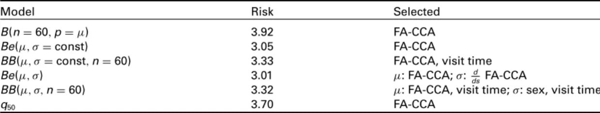
Since it is unclear which distribution is the most appropriate for modelling the PASAT scores, we compare model fit and selected terms for binomial, beta and beta–binomial models, as well as a (distribution-free) median regression model. For the beta and beta–binomial models, we investigate models that model only the expected value as well as those that also feature an additional additive predictor for the dispersion parameter.
Optimal stopping iterations for each model are determined by evaluating the out-of-bag risk for 100 bootstrap samples of the data. Since the risk function that is minimized for these models is simply the negative log–likelihood of the respective model, we can determine the most appropriate distributional assumption