Alma Mater Studiorum
Universit`
a degli studi di Bologna
Department of Electronics, Computer Science, and Systems
Scuola di Dottorato in Bioingegneria - Ciclo XXIII Settore scientifico disciplinare di afferenza: ING-INF/06
Methodological improvement of
3D fluoroscopic analysis for the robust quantification of 3D
kinematics of human joints
presented by
LucaTersi
Supervisor
Prof. AngeloCappello
Co-supervisors
RitaStagni, Ph.D. SilviaFantozzi, Ph.D.
Reviewers
Prof. MarioCesarelli Prof. VasiliosBaltzopoulos
Ph.D. Coordinator
Prof. Angelo Cappello
ABSTRACT
3D video-fluoroscopy is an accurate but cumbersome technique to estimate nat-ural or prosthetic human joint kinematics. This dissertation proposes innovative methodologies to improve the 3D fluoroscopic analysis reliability and usability.
Being based on direct radiographic imaging of the joint, and avoiding soft tissue artefact that limits the accuracy of skin marker based techniques, the flu-oroscopic analysis has a potential accuracy of the order of mm/deg or better. It can provide fundamental informations for clinical and methodological appli-cations, but, notwithstanding the number of methodological protocols proposed in the literature, time consuming user interaction is exploited to obtain con-sistent results. The user-dependency prevented a reliable quantification of the actual accuracy and precision of the methods, and, consequently, slowed down the translation to the clinical practice. The objective of the present work was to speed up this process introducing methodological improvements in the analysis.
In the thesis, the fluoroscopic analysis was characterized in depth, in order to evaluate its pros and cons, and to provide reliable solutions to overcome its limi-tations. To this aim, an analytical approach was followed. The major sources of error were isolated within-silico preliminary studies as: (a) geometric distortion and calibration errors, (b) 2D images and 3D models resolutions, (c) incorrect contour extraction, (d) bone model symmetries, (e) optimization algorithm limi-tations, (f) user errors. The effect of each criticality was quantified, and verified with anin-vivo preliminary study on the elbow joint. The dominant source of error was identified in the limited extent of the convergence domain for the local optimization algorithms, which forced the user to manually specify the starting pose for the estimating process. To solve this problem, two different approaches
were followed: to increase the optimal pose convergence basin, the local approach used sequential alignments of the 6 degrees of freedom in order of sensitivity, or a geometrical feature-based estimation of the initial conditions for the optimiza-tion; the global approach used an unsupervised memetic algorithm to optimally explore the search domain.
The performances of the technique were evaluated with a series of in-silico
studies and validated in-vitro with a phantom based comparison with a ra-diostereometric gold-standard. The accuracy of the method is joint-dependent, and for the intact knee joint, the new unsupervised algorithm guaranteed a max-imum error lower than 0.5mmfor in-plane translations, 10mmfor out-of-plane translation, and of 3 deg for rotations in a mono-planar setup; and lower than 0.5 mm for translations and 1 deg for rotations in a planar setups. The bi-planar setup is best suited when accurate results are needed, such as for method-ological research studies. The mono-planar analysis may be enough for clinical application when the analysis time and cost may be an issue.
A further reduction of the user interaction was obtained for prosthetic joints kinematics. A mixed region-growing and level-set segmentation method was pro-posed and halved the analysis time, delegating the computational burden to the machine. In-silicoandin-vivostudies demonstrated that the reliability of the new semiautomatic method was comparable to a user defined manual gold-standard. The improved fluoroscopic analysis was finally applied to a firstin-vivo method-ological study on the foot kinematics. Preliminary evaluations showed that the presented methodology represents a feasible gold-standard for the validation of skin marker based foot kinematics protocols.
KEYWORDS
Joint Kinematics 3D video-Fluoroscopy 2D-3D Registration Robust Optimization User Independence ValidationACRONYMS
3DF 3D video-fluoroscopy
ADM Adaptive Distance Map
CT Computer Tomography
DMR Distance Map Resolution
DOF Degree Of Freedom
DRR Digitally Reconstructed Radiography
FOV Field Of View
GA Genetic Algorithm
ISB International Society of Biomechanics
LMA Levenberg-Marquardt minimization Algorithm
MA Memetic Algorithm
MAD Mean Absolute Deviation
MB-RSA Model Based Roentgen Stereo-photogrammetric Analysis (RSA)
MRI Magnetic Resonance Imaging
NURBS Non Uniform Rational B-Splines
STA Soft Tissue Artefact
RMSD Root Mean Square Distance
RSA Roentgen Stereo-photogrammetric Analysis
TKR Total Knee Replacement
CONTENTS
Abstract 3 Keywords 5 Acronyms 7 Contents 9 General introduction 13 Thesis outline . . . 151 Overview: 3D Fluoroscopy Basics 19 1.1 Joint kinematics . . . 19
1.2 3D Fluoroscopy . . . 21
1.2.1 Technical and methodological issues . . . 22
1.3 Pose estimation algorithms . . . 26
1.3.1 Implementation . . . 29
1.4 Conclusions . . . 32
2 Preliminary analysis of the methodological limitations of 3D fluoro-scopic analysis 35 2.1 Introduction . . . 35
2.2 In-silico comparison of mono- and bi-planar 3D fluoroscopy . . . 37
2.2.1 Introduction . . . 37
2.2.2 Methods . . . 37
2.2.3 Results and discussion . . . 40
2.3 In-silico evaluation of the distortion correction in 3D video-fluoroscopy
(3DF) . . . 42
2.3.1 Introduction . . . 42
2.3.2 Methods . . . 44
2.3.3 Results . . . 46
2.3.4 Discussion and conclusions . . . 46
2.4 In-vivo elbow kinematics using fluoroscopy: a feasibility study . . . 49
2.4.1 Introduction . . . 49
2.4.2 Material and methods . . . 51
2.4.3 Results . . . 53
2.4.4 Discussion . . . 55
2.4.5 Conclusions . . . 56
2.5 Preliminary conclusions . . . 57
3 In-silico characterization of the alignment methodology 59 3.1 Introduction . . . 59
3.2 Methods . . . 61
3.2.1 Pose estimation algorithm . . . 61
3.2.2 Algorithm convergence properties . . . 62
3.2.3 Algorithm conditioning . . . 64
3.2.4 Data analysis . . . 64
3.3 Results . . . 65
3.3.1 Sensitivity analysis . . . 65
3.3.2 Distance map resolution . . . 67
3.3.3 Sequential alignment . . . 67
3.3.4 Features . . . 68
3.3.5 Features and sequential alignment . . . 68
3.4 Discussion . . . 71
3.5 Conclusions . . . 73
4 Memetic Algorithms for limitation of misalignments resulting from local minima 75 4.1 Introduction . . . 75 4.2 Methods . . . 78 4.2.1 Memetic algorithm . . . 79 4.2.2 Performance evaluation . . . 83 4.2.3 Data analysis . . . 86 4.3 Results . . . 86 4.3.1 Learning strategies . . . 87 4.3.2 Accuracy . . . 89
Acronyms 11
4.3.3 Precision . . . 91
4.4 Discussion . . . 91
4.5 Conclusions . . . 95
5 In-vitroquantification of the performance of the improved procedure 99 5.1 Introduction . . . 99
5.2 Material and methods . . . 103
5.2.1 Data acquisition . . . 103
5.2.2 Pose estimation algorithms . . . 103
5.2.3 Data reduction . . . 108 5.3 Results . . . 111 5.3.1 Bi-planar . . . 111 5.3.2 Mono-planar . . . 111 5.4 Discussion . . . 112 5.5 Conclusions . . . 113
6 Automation of the segmentation procedure: application to prosthetic components 115 6.1 Introduction . . . 115
6.2 Material and Methods . . . 118
6.2.1 Segmentation algorithm . . . 118 6.2.2 Performances evaluation . . . 121 6.3 Results . . . 125 6.3.1 In-silico . . . 125 6.3.2 In-vivo . . . 130 6.4 Discussion . . . 130 6.5 Conclusions . . . 133
7 3D video-fluoroscopy for the quantification of 3D foot kinematics: a preliminary study 135 7.1 Introduction . . . 136
7.2 Material and methods . . . 139
7.2.1 Data acquisition . . . 139
7.2.2 Functional models definition . . . 140
7.3 Results . . . 140
7.4 Discussion . . . 141
7.5 Conclusions . . . 141
A The FluoroTrack software: user guide 147
A.1 Introduction . . . 148
A.2 Typical analysis workflow . . . 148
A.2.1 Distortion correction . . . 148
A.2.2 Foci calibration . . . 150
A.2.3 Setting the scene . . . 151
A.2.4 Alignment . . . 153
A.3 Other Tools . . . 155
List of Figures 157 List of Tables 159 Bibliography 161 Scientific Writing 175 Journal Articles . . . 175 Conference Papers . . . 175 Awards . . . 177
GENERAL INTRODUCTION
T
hereliable quantification of in-vivo physiological human joint kinemat-ics is fundamental for essential orthopaedic clinical applications such as (a) the development of quantitative diagnostic tools [1], (b) the evalua-tion of surgery outcomes [2], or (c) the characterization of innovative prosthesis designs [3]. Moreover, from a biomechanical and methodological point of view, (d) the validation of non-invasive skin-marker based techniques [4] and (e) the soft-tissue artefact modeling [5] cannot be accomplished without a direct mea-surement of the bones or prosthesis components motion.The discovery of X-ray production and detection technology, made by W.C. Roentgen in 1895 [6], opened the door to the development of innovative investiga-tion techniques capable of visualizing the internal structures of the human body. The development of the X-ray image intensifier and of the television camera in the 1950s allowed the light produced by a fluorescent screen sensitive to the X-ray to be amplified, recorded and monitored. Being based on low X-ray dose, the new technique, known asfluoroscopy, was capable of the real time visualization not only of the internal body structures, but also of their motion. Fluoroscopy is currently applied in various clinical fields such as (a) in orthopaedic surgery, to guide fracture reduction and the placement of metalwork [7]; (b) in the an-giography of leg, heart and cerebral vessels [8]; or (c) during the implantation of cardiac rhythm management devices [9].
The qualitative visualization provided by fluoroscopy, however, is not enough for the quantification of the motion. The step from a 2D qualitative imaging analysis to a 3D quantitative methodology needs a great interdisciplinary work which encompasses together knowledges proper of biomechanical, computer
vi-sion, mathematical and medical sciences. The first achievements arrived with the landmark-based radiostereometric analysis [10], and model-based methods have been proposed since the middle of the 1990s: the knowledge of the 3D shape of a non symmetric object and of one or two radiographic projections were claimed to be enough to estimate the position and the orientation of the object in the space, and thus to reconstruct the object kinematics [11]. In the following years different versions of the technique were developed and generically called
3D video-fluoroscopy (3DF) [12]. A part from differences in the implementa-tion of the alignment algorithm, The fluoroscopic methods are mainly divided into two categories: the mono-planar methods [12, 13], which investigate a big volume with a low X-ray dose, and the bi-planar methods [14], more accurate but invasive and expensive. Both mono-planar and bi-planar methods were ini-tially applied to quantify the total knee replacement kinematics [15], but recent innovations led also to the study of intact joints [16].
The advantages of 3DFare manifold. The direct analysis of bones and pros-thesis motion avoids the soft tissue artefact which limits the reliability of skin-marker based methods [4]. 3DF can theoretically achieve a millimeter/degree accuracy level [17] in joint motion analysis and modern fluoroscopes can work at a frame rate of 10−50 f ps. The dynamic performances are then sufficient to analyze the motion during activities of daily living, and simple joint-specific tasks that can be performed inside the fluoroscopic volume. The performance of 3DFwere frequently exploited for research purposes, but several limitations prevented its use in the common clinical practice.
The alignment algorithms, in fact, is based on a cost function optimization. The optimization is negatively affected by local optima that are caused by the morphological symmetries of the investigated model, by cluttering of the con-tralateral limb, or by image blurring, which often interfere with the correct pose estimation [18]. Being prone to errors caused by the detection of false poses, a long time consuming user interaction is required to align the 3D model of the segment to the relevant fluoroscopic projections and to get as close as possible to the real pose. The manual alignment is followed by a 2D-3D registration algo-rithm aimed at the refinement of the results, but the outcome of the procedure remains strongly operator dependent [19].
Besides the technical limitations, it must be pointed out that the fluoroscopic examination implies an ionizing radiation dose for the patient [20]. Its inva-siveness was reduced with the recent researches, but the dose may exceed the
Introduction 15
normative limits when a bi-planar setup is used in combination with computer tomography (to get the 3D model of the joint). The risks correlated to any clinical investigation, must be justified by the outcome of the procedure. Physicians may be reluctant to adopt these radiologic methods even if3DFcan provide exclusive indications about the physiological and pathological behavior of the joints.
All together, the long user interaction, the computational burden, and the invasiveness, slowed down the translation of3DFfrom the research to the clinic.
The goal of the current Ph.D. project is then to introduce method-ological improvements in the 3D fluoroscopic analysis to make it more robust and reliable. To this aim, an analytical identification of the various sources of error was carried out, investigating solutions to im-prove the reliability of the results and to automate and speed up the data analysis.
The achievement of these objectives will lead to a more mature and user friendly technique, in which the user interaction is reduced and the cumbersome data analysis is delegated to the machine. A reliable mono-planar method will also halve the radiation dose for the patient fostering the use of the technique in the clinical practice. Moreover, finding out the limits and the possibilities of
3DFis a fundamental step necessary to define appropriate joint and pathology specific acquisition and elaboration protocols.
The Ph.D. activities were structured as follow: after an analysis of the state of the art for the quantification of human joint kinematics, preliminary analyses were carried out in order to find out the major limitations of3DF; solutions were proposed to improve the analysis in term of accuracy and robustness and in-silico andin-vitro validation were carried out to quantify their performance; the technique was then applied as a gold-standard for a preliminary methodological validation study of stereophotogrammetric protocols for the quantification of foot kinematics. Finally, as a further automation improvement, a semi-automated prosthesis segmentation protocol was proposed and evaluated.
Thesis outline
Chapter1resumes the basic information of the state of the art about the methods for quantification ofin-vivo joint kinematics, clarifying their pros and cons. Two radiographic methods are discussed: Roentgen Stereo-photogrammetric Analysis (RSA), which excels in accuracy, and 3D video-fluoroscopy which emerges as an
optimal compromise between accuracy and invasiveness. The technical issues correlated to the use of the techniques and details about the implementation of the 3D alignment algorithm are presented.
Three preliminary works are discussed in Chapter2, and were meant to iden-tify the points of strength and the potentially improvable limitations of the 3D fluoroscopic analysis. Two of these were in-silico evaluations carried out to in-vestigate whether the image distortion correction and the calibration procedures were effective, and to evaluate the performances of the mono-planar analysis as compared to the bi-planar. The third study aimed at the evaluation of 3DF
when dealing within-vivo datasets. It was found out that the errors related to the bone morphology and symmetries cannot be avoided because intrinsic to the analyzed segment, but it must be quantified to characterize the joint-dependent performances of3DF. It is possible, on the other hand, to improve quality and robustness of the optimization algorithm which is used to estimate the pose.
The3DFversions proposed in the literature before the current Ph.D. activity used a local optimization algorithm. In Chapter 3, a sensitivity analysis was carried out to describe the convergence properties of the algorithm, and two solutions were proposed to enlarge the global optimum basin of attraction: the first consisted in the sequential alignment of the degrees of freedom in order of sensitivity, and the second consisted in estimating the pose optimization initial guess using simple geometrical features extracted from the fluoroscopic images.
A further improvement of the pose estimation algorithm robustness was intro-duced in Chapter4. A hybrid memetic algorithm was designed merging together the improved local search developed in Chapter3and a global genetic algorithm. Anin-silicoevaluation was carried out in order to evaluate accuracy and precision of the new robust method, and it was demonstrated that the memetic algorithm can provide excellent results even without the supervision of the user.
The new algorithm was finally evaluated with the phantom based validation study described in Chapter5. Due to the absence of non-invasive gold-standards, thein-vivo validation of 3DF is not feasible. On the other hand, the accurate marker based RSAcould be used as an in-vitro gold-standard for the quantifi-cation of the kinematic of a knee phantom joint. Differently from the analysis of Chapter2, the performance of the mono-planar and bi-planar3DFwere com-pared considering a real setup and thus including all the sources of error of the analysis. The study was carried out in collaboration with the Laboratory of Move-ment Analysis and MeasureMove-ment (LMAM) of the Ecole Polytechnique F´ed´erale
Introduction 17
de Lausanne, Switzerland (EPFL, Lausanne, Switzerland) and the acquisitions were made at the Centre Hospitalier Universitaire Vaudois (CHUV).
A further improvement towards the automation of 3DF was illustrated in Chapter 6. Many fluoroscopic methods rely on the contours extraction of the segment of interest in the fluoroscopic images. The procedure is typically car-ried out with a time consuming manual elaboration. If little can be done for the segmentation of intact joint bones, on the other hand the segmentation pro-cess can be automated for prosthesis analysis. In fact, even if 3DFwas widely applied to prosthesis kinematics, it is still necessary to characterize thein-vivo
behavior of new prosthesis design. A new semi-automated method for prosthesis segmentation in3DFwas proposed. The method was developed and validated in collaboration with the DEIS Bioimaging group of the University of Bologna.
Once validated, the improved method was finally applied to thein-vivo foot and ankle kinematics as described in Chapter 7. The great clinical interest of this joint is demonstrated by the number of stereophotogrammetric protocols recently proposed, which, like any marker-based protocol, are prone to accu-racy limitations due to soft tissue artefact and to the deformability of the foot throughout the gait cycle. 3DFcan accurately quantify the foot kinematics in physiological conditions, without limitations to range of motion and skin sliding, and could serve as a gold-standard for the validation of the stereophotogram-metric protocols. On the other hand, due to the small size and the symmetries of the involved bones, the hind-, mid- and fore-foot must be analyzed as com-pound segments. These segments, however, are intrinsically deformable, and the quantification of their accurate relative kinematics needs function-related mod-els. A fluoroscopic gold-standard based on a functional-anatomical model for the assessment of marker-based foot protocols was proposed. Synchronous stereopho-togrammetric and fluoroscopic acquisitions of foot kinematics were carried out, and the model was applied to quantify the gold-standard kinematics to validate the stereophotogrammetric foot protocol. This preliminary study was carried out in collaboration with the University of Padua (Italy).
All the analysis were carried out with the newly developed software called FluoroTrack described in appendixA. The software was designed to be a com-prehensive framework for the complete 3DF analysis. The software included toolboxes for (a) 3D visualization, (b) image processing, (c) model and marker based mono- and bi-planar 2D-3D registration algorithms, (d) anatomical refer-ence frame definition, (e) structured simulations and data analysis.
CHAPTER
ONE
OVERVIEW: 3D FLUOROSCOPY BASICS
1.1
Joint kinematics
Reliable knowledge of in-vivo joint kinematics, in physiological conditions, is fundamental for various clinical applications: (a) the study of prosthesis design must aim at the replication of intact joint biomechanical function [3,21], (b) the development of quantitative diagnostic tools can help the detection of patho-logical alterations in motion [1], and (c) the outcomes of orthopaedic surgery must be quantified to find correlation with the recovery of physiological joint motor activities [2, 22]. Moreover, from a methodological point of view, ac-curate methods are necessary to validate and to evaluate errors associated with non-invasive techniques for the quantification of motion (i.e. inertial sensors, stereo-photogrammetry [5]).
For validation purposes, a gold-standard technique is needed to obtain accu-rate bone motion data directly avoiding Soft Tissue Artefact (STA). As testified by validation studies to test the protocols repeatability [23,24,25], and accuracy [26, 27,28], STAis the major source of error for marker based protocols. STA
leads to errors in joint translations and rotations of some centimeters and several degrees, respectively [4, 29,30]. Moreover, segments such as the foot, the fore-arm, or the hand are composed by intrinsically deformable sub-segments. Skin marker based protocols treat these segments as rigid, introducing further errors in the kinematics estimation.
Cadaver studies can lead to accurate kinematics quantification [27, 31] but these kind of evaluation can hardly represent the clinically operativein-vivo con-ditions: furthermore, it is difficult to expand the approach for the evaluation of new protocols. When bone kinematics reconstructed using markers applied on the skin and on rigid plates were comparedin-vivo with the one obtained from intra-cortical pins [26], it was not possible to acquire all the measurements simul-taneously due to the limited dimension of the Field Of View (FOV). Thus, the results can be considered valid under a strict hypothesis of motor task repeata-bility, and even a simultaneous acquisition would underestimate STA, because pins limit skin motion. Moreover, although the use of intra-cortical pins allows one of the best accuracy, it cannot be adopted for human tests [26, 32, 33] for obvious ethical reasons, skin movement limitation and possible kinematics alter-ation. Less recently, using radiologic techniques that do not limit skin motion,
STAwas evaluatedin-vivo in the foot, but the performed analysis was only 2D [28].
Radiostereometry or Roentgen Stereo-photogrammetric Analysis (RSA), de-signed for the quantification of prostheses components fixation [34,35], was also used forin-vivo joint kinematics [36], but it is highly invasive as it is based on traditional X-rays and requires surgical intervention for radiopaque markers im-plantation. Finally, techniques based on computer axial tomography or magnetic resonance [37, 38, 39] have a small field of view, and a frame rate not sufficient for dynamic tests without combining data from a sequence of cyclic repetitions.
The best compromise among low invasiveness, high accuracy of dynamic anal-yses and flexibility was found by Banks et al. using a mono-planar fluoroscopic technique [12]. This technique was initially applied to prosthetic joints, exploiting the prosthetic implant radiopacity, that is highly contrasted even in fluoroscopy. Limiting X-rays exposure, it is possible to tune a trade-off between spatial and temporal resolutions of the analysis. This technique, denominated 3D video-fluoroscopy (3DF), was extended later to intact joint, requiring Computer To-mography (CT) [40] or Magnetic Resonance Imaging (MRI) [41] scan of the bony segments for the estimation of bone surface geometry.
In the following sessions, the principal fluoroscopic methodologies for the quantification of human joint kinematics will be described and compared.
1.2 3D Fluoroscopy 21
1.2
3D Fluoroscopy
To overcome the marker-based RSA practical limitations such as the surgical implantation of tantalum beads on the bone surface, or the use of double high X-ray dose radiologic projections (see Chapter 5), model based methods were proposed. The knowledge of 3D geometry of joint segments, and mono- or bi-planar projection views in fluoroscopic images, were claimed to be sufficient to reconstruct the absolute and relative 6 Degrees Of Freedom (DOFs) pose of bones or prostheses in the 3D space.
3D video-fluoroscopy (3DF) is a technique for the evaluation of joint kine-matics based on the alignment of 3D models of bones or prostheses and series of 2D radiographic images representing the relevant mono-planar or bi-planar projections [42]. The joint kinematics is reconstructed estimating, independently for each video-frame, the 6DOFs absolute pose (3 translations and 3 rotations) of each body segment, and then calculating the 6DOFs of their relative pose.
3DFcould provide reliable knowledge about joint kinematics, because it the-oretically permits to achieve a millimeter/degree accuracy level in joint motion analysis [12,43], with relatively high dynamic performances (up to more than 50 fps with modern fluoroscopes). These performances are sufficient to analyze the motion during activities of daily living, and simple joint-specific tasks that can be performed inside the fluoroscopic volume (1.1).
In-vivo knee tasks, such as squat, stair climbing, chair raising and sitting or step up-down, were widely analysed with 3DFin replaced [13, 15, 44, 45] and intact knee [40]. 3DFwas also applied to quantify thein-vivo kinematics of ankle [46] and hip [47,48] joints.
For the accuracy level and the possibility to acquire relatively fast dynamics,
3DFwas used as a gold-standard in methodological studies for the validation and the evaluation of error associated with non invasive techniques for the quantifi-cation of motion. For the first time, acquiring simultaneously fluoroscopic and stereo-photogrammetric data, Stagni et al. [4] quantified soft tissue artefact at the thigh and shank without constraint to skin motion, and evaluated the error propagation to the resulting knee kinematics. Successively, these data allowed to analyze another source of error in stereo-photogrammetry such as anatomi-cal landmarks mislocation [49] and to compare the performance of differentSTA
compensation methods [50].
video-fluoroscopy, a 3D model of the bone is virtually moved until it is best aligned to the relevant 2D image. This automatic procedure is typically carried out by means of an iterative optimization algorithms. Different metrics have been used to quantify a cost or a fitness function for the optimization such as: (a) the euclidean distance between the contour of the virtual projection of the model and the contour extracted from the fluoroscopic image [12, 51], (b) the root mean square distance between the projection lines and the model surface [3], (c) similarity measures between the fluoroscopic image and digitally reconstructed radiographies [52,53,54,55,56].
Promising accuracy levels have been reported for the intact knee joint: 0.23mm
for translation, 1.2degfor rotation with bi-planar fluoroscopy [55]; and 0.42mm
for in-plane and 5.6 mm for out-of-plane translations, 1.3 deg for rotation for mono-planar fluoroscopy [17]. However, these accuracies cannot a-priori be con-sidered valid and generalized for the other joints due to differences in the bone morphology and anatomy.
1.2.1
Technical and methodological issues
The performance of 3DF were frequently exploited for research purposes, but several limitations prevented its use in the common clinical practice.
The performance of3DF, in fact, is affected by the geometry of the bone seg-ments analyzed, and its accuracy could vary considerably because local minima, caused by symmetries of the models surfaces, or by occlusions, could severely in-terfere with a correct estimation of the pose. The alignment algorithms, in fact, is based on a cost function optimization. The optimization is negatively affected by the local optima that characterize the multivariate objective function. The local optima are caused by several factors:
the investigated bones and prosthesis are often characterized by morpho-logical cylindrical and spherical symmetries, and their projections may not be biunivocally related to their 3D poses;
when analyzing cyclic tasks such as walking, it is common that the con-tralateral limb clutters the fluroroscopic projection of the investigated limb;
the moderate sensitivity of the phosphors to the X-rays imposes lower limits to the shutter speed of the acquisition system, which in turn often introduce image blurring (and contours smoothing) when acquiring limbs in motion.
1.2 3D Fluoroscopy 23
Cluttering and blurring contribute in perturbing the informations needed to prop-erly quantify the objective function for the optimization. Moreover, fluoroscopic images are geometrically distorted. If not properly compensated, the distortion may introduce errors in the calibration process and may deform the objective function. Methods for the image distortion correction are discussed in the next section.
Being prone to errors caused by the detection of false poses, a long time consuming user interaction is required to align the 3D model of the segment to the relevant fluoroscopic projections and to get as close as possible to the real pose. The 2D-3D registration algorithm become then a mere refinement of the results, but the outcome of the procedure remains strongly operator dependent. To significantly improve the quality and the robustness of 3DF, it is then necessary to understand how the various sources of errors on affects the alignment algorithms and the final accuracy of the pose estimations. For this purpose, an analytic approach was adopted in order to find appropriate solutions to each single defect of the method.
Calibration and distortion correction
X-Ray Image Intensifier (XRII) systems are commonly used for digital planar image acquisition in radiology. However, even the best XRII system hardware cannot deliver images free of artefact. Lag, vignetting, veiling glare, geometrical distortions are introduced. A recent change in the fluoroscopic technology from
XRII to flat panels, improved the quality of the acquired images, reducing the artefacts and increasing the sensitive to the X-rays, allowing thus the reduction of the intensity of the emitting radiations [20]. Due to the low cost,XRIIis however still common in the clinics, and the artefacts must be taken in consideration to develop quantitative fluoroscopic techniques.
Lag Lag is the persistence of luminescence after X-ray stimulation has been terminated. Lag degrades the temporal resolution of the dynamic image. Tra-ditionalXRII tubes have lag times of approximately 1 msec. Therefore, lag in modern fluoroscopic systems is more likely caused by the closed-circuit television system than by theXRII.
Vignetting A fall-off in brightness at the periphery of an image is call vi-gnetting. Vignetting is caused by the unequal collection of light at the center of
theXRII compared with light at its periphery. As a result, the centre of aXRII
has better resolution, increased brightness, and less distortion.
Veiling glare Scattering of light and the defocusing of photoelectrons within theXRII are called veiling glare. Veiling glare degrades object contrast at the output phosphor of theXRII. As mentioned, the contrast ratio is a good measure of determining the veiling glare of anXRII. X-ray, electron, and light scatter all contribute to veiling glare.
Geometric distortion With ordinary sizes of the XRII, the images are af-fected by geometric distortion which causes a variation in magnification up to 5%-10% [57]. The geometric distortion has two main sources: the projection of the X-ray beam onto the curved input surface of theXRII and the deflection of the electrons inside theXRII caused by any external magnetic field. The former produces the typical “pincushion” distortion. The latter source may produce a sigmoidal distortion if the orientation of theXRII is parallel to the external magnetic field [58]. Larger XRIIare more sensitive to the electromagnetic fields, causing a larger sigmoidal distortion.
Fluoroscope systems allow for the observation and analysis of biological struc-tures, which could not be seen from outside in other ways. The images obtained with this instrument are geometrically distorted and unsuitable for a quantitative analysis, unless a careful correction procedure is performed. To characterize the geometric distortion of the specificXRII used, an image of a rectilinear calibra-tion grid placed on the input screen of theXRII is commonly used. Analytical function are used to map distorted positions to undistorted positions. This is performed either locally for each quadrilateral or triangular patch [59] identified by four or three grid points respectively, or globally [60, 61]. Local techniques produce discontinuities from one patch to the other [62]. The global technique based on polynomials [60] avoids discontinuities and are more accurate than the local techniques, and were used in the present study.
The pixel spacing is also determined with this procedure, and through the acquisition of a second calibration device typically a 3D cage of Plexiglas with tantalum balls in known positions, the position of the X-ray source [63], and the eventual relative position of the second fluoroscope could be estimated minimizing the Euclidean distance between the projection of a model of the cage and the positions of the markers center in the distortion corrected fluoroscopic image.
1.2 3D Fluoroscopy 25
Vignetting compensation A simple approach can be used to compensate for vignetting in fluoroscopic session. According to the Lambert-Beer law, in fact, at a first approximation, each pixel gray level is proportional to
Ii,j=Ii,j0 e− R
Ωαi,j(x)dx withi, j= 1, . . . ,1024 (1.1)
WhereI0 is the intensity of the emitted X-ray,α(x) is an absorption coefficient, and the integral is along the extent Ω of the absorbing tissue the ray passed through. A gradient inI0 is a disturbing factor, origin of the vignetting effect. On the other hand, in a fluoroscopic session, the fluoroscope parameters usually are not modified throughout the acquisition. It is then possible to acquire an empty image representing the intensity of the light fieldI0. The light gradient can than be compensated computing the intensity of each pixelGi,j as:
Gi,j= Z Ω αi,j(x)dx= ln I 0 i,j Ii,j ! withi, j= 1, . . . ,1024 (1.2)
which is a quantity proportional to the density and to the thickness of tissue the emitted ray passed through.
Ionizing radiation dose
Besides the technical limitations, it must be pointed out that the fluoroscopic examination implies an ionizing radiation dose for the patient [64].
As for any radiological investigation technique, the risk correlated to radiation exposure must be taken into account to properly evaluate the trade off between the significance of the outcome of the procedure and its invasiveness. In Italy, the radiation exposure is regulated by the decree D.Lgs. 230/95 [65].
The biological effects of radiation is reflected by the dose equivalent, which is measured in sievert (Sv) by the SI. It is equivalent to the absorbed dose (measured in gray Gy) multiplied by a conversion factor which depends on the kind of radiation. The X-ray conversion factor is equal to 1. Another non SI unit of measurement to describe the dose is the roentgen (R) for which the following relation is valid: 1R= 0.12Sv .
The annual dose was classified [66] as: low (≤ 3 mSv), moderate (> 3 to 20 mSv), high (> 20 to 50 mSv), or very high (> 50 mSv). For the health-care professionals the following limits have been fixed: maximum total dose of
100 mSv in five consecutive years, with a further limitation of a maximum of 50mSv in one year. For the common people the limit was fixed at 1 mSv per year.
For the in-vivo acquisition described in Chapter 7, the fluoroscopic system Sirecon 40hd (Siemens) declared a dose of 4.8µRper image. A total number 600 frames were acquired at 6 f ps, corresponding to 3000 µR which are equivalent to 0.36mSv, approximately one third of the annual limit. Moreover, this value correspond to the emitted dose while the skin absorbed dose would certainly be lower. On the other hand, increasing the acquisition frame rate and using a bi-planar setup, the ionizing dose for the patient will certainly increase, eventually reaching harmful limits if combined to other radiological based examination such as aCTto acquire the 3D model of the bones. To be on the side of safety for a possible clinical application, it is advisable to useMRIinstead ofCTand mono-planar fluoroscopic setup, but an interslice spacing of less than 1mmis needed to assure a good resolution of the model.
1.3
Pose estimation algorithms
All the fluoroscopic methods for the quantification of joints kinematics estimate the pose of the investigated object for each of the acquired frames. The meth-ods are mainly divided into two categories: the mono-planar methmeth-ods, which investigate a big volume with a low X-ray dose, and the bi-planar methods, more accurate but invasive and expensive (Figure1.1). Both mono-planar and bi-planar methods were initially applied to quantify the total knee replacement kinematics, but recent innovations led also to the study of intact joints.
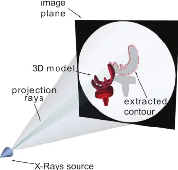
In 3D joint kinematics with3DF, the accurate knowledge of the geometry of the bony or prosthetic segments is necessary together with the relevant projection on the image plane. When a non-symmetric object is imaged by a nonorthogonal camera, a unique projection is produces for each 3D pose of the object. The pose estimation of the bone from a single view can be obtained by aligning the 3D object model in order to obtain a corresponding projection as observed in the X-ray image. A perspective projection model can represent the fluoroscope. In perspective projection model, a pinhole camera forms the image. X rays are considered straight lines emitted by a point source of uniform radiation in all directions (Figure1.2). X-rays pass through the object damping their intensity according to the Lambert-Beer law (equation1.1), and this process can be
vir-1.3 Pose estimation algorithms 27 Image intensifier and camera 3D imaging area X-Ray source and collimator X Y Z A) B)
Figure 1.1: Configuration of a mono-planar (A) and bi-planar (B) fluoroscopic system. The bi-planar is more reliable but can investigate smaller volumes (in light red) with a higher X-ray dose for the subject.
tually simplified and replicated in order to estimate the pose that generated the real fluoroscopic image.
Mono-planar methods The first model based method in the literature was proposed by Banks and Hodge in 1996 [12]. An object recognition technique presented by Wallace and Wintz [67] formed the basis for the shape represen-tation and matching components of the pose estimation process. Contour sil-houettes were represented by normalized Fourier descriptors, where each contour was normalized for in-plane translation, in-plane rotation, and scale. The results indicated that knee rotations could be measured with an accuracy of approxi-mately one degree and that sagittal plane translations could be measured with an accuracy of approximately 0.5 mm, but the technique was not reliable for the out-of-plane pose parameters. However this method could be applied only to prostheses, relied on the creation of a contour library of the object in different sampled poses, and had to interpolate the results for the inter-sample cases.
A similar approach was used by Hoff and Stiehl [43,51] with different represen-tations of silhouettes and alignment algorithm. Being based on the comparison of the areas of the prosthesis, these techniques had to extract closed curve contours, and this is not always possible in fluoroscopic images mainly due to cluttering.
technique, described in depth in Section 1.3.1 exploit the algorithm proposed by Lavall´ee and Szelinsky [11]. This algorithm is based on tangency condition between the model 3D surface and the projection rays that generated the external contours of the object in the image. Differently from the previous methods, this algorithm could work also with incomplete contours.
To reduce the user interaction, Mahfouz et al. [13] proposed a contour match-ing method that does not need manual identification of the external contours but exploit also the information of the internal part of the images. Informations re-lated to spurious contours, however, interfere with a proper alignment reducing the convergence domain of the real pose.
Bi-planar methods To improve the accuracy of3DFin the estimation of the out-of-plane pose parameters, different bi-planar methods were proposed.
Tashman and Anderst [68] used for the first time a bi-planar setup, but due to the high radiation dose, the method was test on a canine intact knee. The matching was carried out optimizing a similarity metric between a Digitally Re-constructed Radiography (DRR) and the relevant real projection. For the 3D model generation aCTacquisition was needed. The method was applied to the human knee in 2007 [2], and validate versus aRSAgold-standard with an invasive study during a running task. The declared accuracy was of 0.15−0.52mmand 0.34−1.27degdepending on the DOF.
Bingham and Li [69] proposed a new alignment algorithm calledconnectivity method which is a contour matching methods between the extracted contour in the image and the iteratively created virtual contour of the prosthesis. The declared accuracy is in the order of 0.2mm/deg.
Another solution was proposed by Kaptein in 2003 [14]. Using reverse engi-neering 3D models of prostheses and contour matching methods in a phantom based validation study, a maximum standard deviation of the error in the migra-tion calculamigra-tion of 0.14mmfor translations 0.05degfor rotation.
Even if bi-planar fluoroscopy is more robust and accurate, the present work focused on mono-planar fluoroscopy because it can investigate bigger volume with smaller X-ray dose for the patient. Moreover, mono-planar fluoroscopy represents the worst case scenario, more suitable to highlight and identify the pitfalls of the method and to optimize the pose estimation in terms of accuracy and precision. In the present work, a modified version of the pose estimation algorithm
1.3 Pose estimation algorithms 29
proposed by Lavall´ee and Szelinsky [11] and based on Adaptive Distance Maps (ADMs) was implemented. This algorithm was chosen because of its light com-putational weight and because it permits to achieve good accuracies even with incomplete contours [3], which can arise from occlusions or image blurring due to the bone motion.
X-Rays source
3D m odel
extracted
contour
projection
rays
image
plane
Figure 1.2: Virtual representation of a fluoroscopic system for the pose estima-tion with tangency condiestima-tion
1.3.1
Implementation
An established technique was implemented to estimate the 3D pose of an ob-ject of known 3D geometry given its mono-planar fluoroscopic proob-jection [3]. The algorithm was originally proposed by Lavall´ee and Szeliski [11] for bi-planar projection, and it is based on 3D ADM. In brief, (a) the fluoroscope is virtu-ally modeled with a perspective projection model; (b) the 3D pose estimation is obtained with an iterative procedure that finds the best alignment between a bone surface model and its 2D fluoroscopic projection (typically a 1024x1024
DICOM1image). In the present study, the bone surface was modeled with
tri-angles meshes, however different representation can be used (i.e. cloud of points, Non Uniform Rational B-Splines (NURBS)).
The quality of the alignment is represented by a cost function defined as:
RM SD(p) = v u u t 1 n n X i=1 [d(Sm(p), li)]2 (1.3)
RMSDis the root mean square distance between the surfaceSm(p) of the model mpositioned in the posep= (Tx, Ty, Tz, Θx, Θy, Θz) andnprojection linesl. The projection lineslrepresent the X-rays that generated the edge points of the bone segment projection extracted by a Canny edge detector [70] in the fluoroscopic image and is expressed in parametric form:
li:Ci+λ·
F−Ci
Li
, λ∈[0, Li] (1.4)
WhereF = (F x, F y, F z) is a point representing the X-ray source position (focus),
Ci= (Cix, Ciy, Ciz) is thei−thof thenpoints of the contour, both expressed in the fluoroscopic system of reference, andLi is their distance:
Li=kF−Cik (1.5)
To quantify the Root Mean Square Distance (RMSD),liis sampled and, for each sampling pointPki=li(λk), the distance from Sm(p) is computed. The distance of the projection line from the surface is then defined as the minimum distance among those of the line sampling points.
d(Sm(p), li) = min k d(Sm(p), Pki) (1.6) The best alignment condition is finally identified finding the values of the posep
that minimize theRM SDwith an optimization algorithm.
RM SDmin= min
p [RM SD(p)] (1.7)
For a faster quantification of the distanced(Sm(p), li) between the line and the
1.3 Pose estimation algorithms 31
model surface, and to define the sampling step ofli,ADMs of the model surface is pre-computed and stored.
Figure 1.3: Adaptive Distance Maps (ADMs) of the elbow bones.
Briefly, the ADMis an octree-based representation of an object [71]. In this representation, the volume outside and inside the surface of the object is non-uniformly discretized. The map assigns to each point of the discretization the corresponding signed distance from the surface of the model: positive if outside, negative if inside the object.
The distance is computed as the minimum distance between the discretization point and the surface of model of the bone. The structure of theADMis an octree which is built with an iterative procedure which subdivides a cube (also called octant) iteratively in other 8 half-side octants only if it contains at least one point of the mesh. The octree is then refined to avoid discontinuities between the levels of subdivision of two adjacent octants. The vertices of the octants are the volume discretization points. The distance of a generic point from the surface is then computed with a tri-linear interpolation of the distances of the 8 vertices of the smallest octant containing the point. The octant side dimension gets smaller closer to the surface, thus the interpolation error becomes negligible. In the present work, the resolution of the octree (smallest octant side) will be referred as Distance Map Resolution (DMR). For a further improvement of the algorithm speed, also the sampling step of the projection lines is adaptive. The sampling step varies accordingly to the local resolution of the ADM and gets
smaller closer to the surface. If si
k is the side of the smallest octant containing
the sampled pointPki then the next point to evaluate the distance will be:
Pki+1=li(λk+1); λk+1=λk+
si k
2 (1.8)
Finally, li is resampled around the closest point to the surface with a uniform
step length ten times smaller thanDMR.
V1 V2
V3 V4
P
Figure 1.4: Scheme of the projection ray sub-sampling procedure. The octree is iteratively subdivided only if it contains at least one point of the model surface. The distance of a generic point P is the trilinear interpolation of the vertices (V) of the smallest octant containing that point. Information of the octant side is used for the adaptive sampling of the projection rays.
1.4
Conclusions
X-rays imaging methods proved to be valuable tools for the quantification of hu-man joints kinematics, but, in order to find a good compromise among reliability, costs and invasiveness, much work can be done.
1.4 Conclusions 33
Even if bi-planar fluoroscopy is more robust and accurate, the present work focused on mono-planar fluoroscopy because, being less robust, it can better high-light the limitation of the fluoroscopic methods. A modified version of the pose estimation algorithm proposed by Lavall´ee and Szelinsky [11] was implemented. This algorithm was chosen because of its light computational weight and because it permits to achieve good accuracies even with incomplete contours [3]. Due to this characteristics, even if developed for prosthetic components, the algorithm can be applied also to natural joints.
The described 2D-3D registration algorithm will be investigated in depth in the following chapters. In particular differentin-silico studies will characterize its performances under controlled conditions, in order to isolate and evaluate the ef-fects of the various sources of error. Considerations will stem indicating the path to follow to improve the robustness and the quality of the measurements, and novel methods will be proposed to overcome the limitations of the current tech-nique. The work will focus on the common aspects of the different3DFmethods such as the distortion correction, the optimization, and the segmentation. The worst case scenarios will be investigated, in order to highlight the limitations. The results will be generalizable to other alignment algorithms.
CHAPTER
TWO
PRELIMINARY ANALYSIS OF THE
METHODOLOGICAL LIMITATIONS OF 3D
FLUOROSCOPIC ANALYSIS
2.1
Introduction
In this chapter the preliminary analysis meant at the investigation of the main limitations related to the use of mono-planar 3D video-fluoroscopy (3DF) for the quantification of human intact and prosthetic joint kinematics will be discussed.
Part of the material described in this chapter was submitted to:
L. Tersi, S. Fantozzi, R. Stagni, A. Cappello: In-vivo elbow kinematics using flu-oroscopy: a feasibility study: Under review to Computer Methods and Programs in Biomedicine.
L. Tersi, R. Stagni, P. Masini, S. Fantozzi, A. Cappello: 3D fluoroscopy to analyse elbow kinematics. Proceeding ofESBME 2008, Crete.
L.Tersi, R. Stagni, S. Fantozzi, A. Cappello: Mono-planar vs Bi-planar 3D Fluoroscopy: in-silico Simulation of the Estimation of Total Knee Replacement kinematics. In: Pro-ceedingsVPH 2010, Brussels, Belgium, September 30 - October 1, 2010
L. Tersi, R. Stagni, S. Fantozzi, A. Cappello: Total Knee Replacement kinematics: an in-silico reliability comparison between mono-planar and bi-planar 3D Fluoroscopy. In: ProceedingsXVII ESB Conference 2010. Edinburgh, Scotland UK, 5-8 July 2010. This work was awarded with theESB Travel Award 2010.
The accuracy of the measure depends on instrumental and environmental factors, such as (a) the number of projections considered, (b) the methodology to correct the geometrical distortions of the fluoroscopic images and (c) the calibration to establish the operating dimensions of the virtual fluoroscope, or (d) the geometry of the bony segments to be reconstructed. Moreover, the lack of a non-invasive gold-standard that can be appliedin-vivo prevents the analysis of the influence of the various sources of error in optimal condition. Thus, in order to obtain a reliable estimation of the intact or prosthetic joint kinematics, computer simula-tions might help to isolate the various sources of error and to find proper specific solutions.
In order to find out to which extent the algorithm proposed by Lavall´ee [11] is suitable for mono-planar projection, anin-silico comparison between the mono-planar and bi-mono-planar 3DF applied to knee prosthesis is proposed. Then the effect of the correction distortion and calibration were investigated with another
in-silico study: using Digitally Reconstructed Radiographies (DRRs) obtained from upper limb CT models, we focused on how the geometric deformation of the fluoroscopic images modifies the estimate of the elbow kinematic. Finally, an
in-vivo preliminary study on the elbow joint is proposed to test the performance of the method on real data.
2.2In-silico comparison of mono- and bi-planar 3D fluoroscopy 37
2.2
Quantification of the performance reduction
from bi-planar to mono-planar 3D Fluoroscopy
2.2.1
Introduction
A better knowledge of the kinematics behavior of Total Knee Replacement (TKR) during physiological activity still remains a crucial issue to validate innovative prosthesis designs and different surgical strategies. X-ray imaging tools for the accurate measurement ofin-vivo kinematics ofTKRcomponents have been used to improve the clinical outcome of knee replacement [47]. The Roentgen Stereo-photogrammetric Analysis (RSA) is currently considered as a gold-standard but invasive technique. It is based on bi-planar X-ray projections and on tantalum beads implants on prosthesis and bone surfaces. To avoid marker implantation, mono-planar fluoroscopic techniques [12] were proposed. Recently, Model Based
RSA(MB-RSA) [72,68,69] were introduced to increase the technique reliability
but with higher costs and invasiveness. The knowledge of the 3D geometry of the components and a mono-planar projection view in a fluoroscopic image were claimed to be sufficient to reconstruct the absolute and relative 6 Degrees Of Free-dom (DOFs) pose of the components with amm/degaccuracy level. However, it is still not clear how the reduction of information introduced by the mono-planar fluoroscopy can affect the accuracy and reliability of the technique. In this in-silicostudy we compared the mono- and bi- planar fluoroscopy, investigating the convergence properties and the sensitivity of the two methods.
2.2.2
Methods
The implemented alignment algorithm was based on 3D surface models and Adaptive Distance Maps (ADMs). Two orthogonal fluoroscopes were represented by perspective projection models (Figure2.1). A global system of reference was defined with thexandyaxis in the image plane of the frontal projection, and the
z axis perpendicular to the image pointing towards the X-ray source, forming a right-hand reference frame. For the lateral projection, the out-of-plane axis wasy. The pose was then estimated minimizing, with a Levenberg-Marquardt minimiza-tion Algorithm (LMA) [73], the Euclidean Root Mean Square Distance (RMSD) between a surface model and a beam of lines connecting the X-ray sources and the edge of the bone extracted in the projected images. A surface model of a
lateral projection frontal projection reference frame prosthesis x-ray sources projection lines x z y
Figure 2.1: Outline of a bi-planar orthogonal setup.
femoral component of aTKR cruciate retaining prosthesis was placed in 4 ref-erence poses and flat shaded projections were generated. The complete contours were extracted and then used for the alignment. The ADMhad a resolution of 0.5 mm.
TheRMSDwith respect to each fluoroscope can be represented as a cusp. Its sensitivity to the variation of theDOFs was then quantified by the slope of the tangents around its minimum varying eachDOFat a time with a step of 0.1mm
or deg (see Section 3.2.2 for details). Different minimizations were carried out varying the initial conditions in the domain around the projection pose. The initial deviation for translations (T) and rotations (Θ) were equal to−4 or 4mm
ordeg, resulting in 256 permutations. Three conditions were analyzed: (a) double projection, (b) frontal projection, (c) lateral projections. The pose estimation errors were quantified and reported in terms of means and standard deviations.
2.2 In-silic o comparison of mono-and bi -planar 3D fluoroscop y -10 -5 0 5 10 10-1 100 101 Tx [mm] RMSD [mm] -10 -5 0 5 10 10-1 100 101 Ty [mm] -10 -5 0 5 10 10-1 100 101 Tz [mm] -10 -5 0 5 10 10-1 100 101 Θx [deg] RMSD [mm] -10 -5 0 5 10 10-1 100 101 Θy [deg] -10 -5 0 5 10 10-1 100 101 Θz [deg]
Frontal Lateral Biplanar
Ph.D.
2.2.3
Results and discussion
TheRMSDsensitivity (RMSD/DOF) was quantified as the slope of the sensitivity curves around their minima, see Figure2.2. With the double projection the sensi-tivity was approximately of the same magnitude for all the translations (medium value'0.34mm/mm), and for all the rotations (medium value'0.09mm/deg). In the frontal and lateral projections, similar results were obtained for rotations, but the sensitivity is larger for the in-plane translations ('0.54mm/mm), and smaller for the out-of-plane translation ('0.01mm/mm). Local minima (high-lighted by the arrow in figure 2.2) are evident for the lateral projection due to the convexities and the symmetries of the model in this projection (see also figure
2.3).
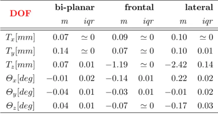
Table2.1reports the means and standard deviations of the pose estimations.
Table 2.1: Median and interquartile range of the estimation error.
DOF bi-planar frontal lateral
m iqr m iqr m iqr
Tx[mm] 0.07 '0 0.09 '0 0.10 '0 Ty[mm] 0.14 '0 0.07 '0 0.10 0.01 Tz[mm] 0.07 0.01 −1.19 '0 −2.42 0.14 Θx[deg] −0.01 0.02 −0.14 0.01 0.22 0.02 Θy[deg] −0.04 0.01 −0.03 0.01 −0.01 0.02 Θz[deg] 0.04 0.01 −0.07 '0 −0.17 0.03
2.2.4
Conclusions
The bi-planar method could always provide errors at least one order of magnitude lower than the mono-planar methods. As confirmed by the sensitivity analysis, the bi-planar method can avoid the low out-of plane sensitivity of one projection relying only on the good information provided by the orthogonal one. As com-pared to the frontal projection, the larger dispersions of the errors obtained in the lateral can be explained by the larger number of convexity (Figure 2.3) in the extracted contours that can cause local minima in the cost function. A
ro-2.2In-silico comparison of mono- and bi-planar 3D fluoroscopy 41
bust minimization algorithm could eventually avoid the minimization problems. The results confirmed the out-of-plane translation is a critical issue in3DF, how-ever error in the order of 1−2 mm could still be acceptable depending on the application.
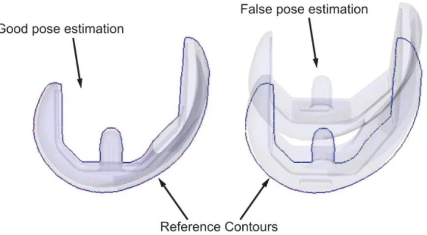
Reference Contours Good pose estimation
False pose estimation
Figure 2.3: False pose estimation due to convexities: the alignment of only one condyle create a local minimum in the cost function.
2.3
In-silico
evaluation of the distortion
correc-tion in
3DF
2.3.1
Introduction
One of the most evident source of error, that makes the step from qualitative to quantitative analysis complicated, is the presence of geometric distortion in the fluoroscopic images. Particular attention must be paid to the calibration of the system and to the correction of any geometric distortions introduced by the image formation chain (Section2.3). Solutions were proposed to deal with the distortion correction and calibration issues [60], and computer aided simulations may help in investigating whether this technique is effective for our particular registration method.
The upper limb is particularly interesting for validation purposes. Recently
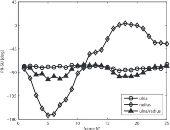
3DFhas been applied to the shoulder [74,75], and the elbow kinematics has been recently investigated with stereophotogrammetric protocols [30, 76]. The elbow plays a fundamental role in activities of daily living such as eating, drinking, cooking, personal hygiene, etc. Any alteration of its anatomical structures can compromise its function. An accurate knowledge of thein-vivokinematics is nec-essary for the development of effective methods for joint surgical reconstruction and rehabilitation.
However, the 2D to 3D mono-planar fluoroscopy registration methods for the estimate of the 6 DOFs pose (3 translations and 3 angles) rely on surface model of the bone to be aligned and are particularly dependent on its spatial symmetries. Moreover, the elbow joint is composed by highly overlapping long cylindrical bones such as radius and humerus, and their alignment can suffer lack of accuracy and reproducibility. The effects of all the sources of error must be related to the final kinematic estimate, and the elbow is a joint that best highlight the problems for the in-vivo application of 3DF. Thus, a thorough validation study is needed to understand whether the proposed method can deal with the difficult alignment of the elbow.
The lack of a non-invasive gold-standard, with an accuracy lower than 1mm
for translations and 1deg for rotations, on the other hand, can complicate in-vivovalidation tests on humans. In-silico analysis are then needed for validation purposes. This study represents the first step towards the characterization of
2.3In-silico evaluation of the distortion correction in 3DF 43
computer assisted simulations. Using Computer Tomography (CT) models of the upper limb bones and constructingDRRs simulating flexion-extension kinematic we investigated (a) whether the algorithm proposed is suitable for the elbow kinematics in absence of significant sources of error, and (b) whether the geometric deformations introduced by X-Ray Image Intensifier (XRII) [60] compromise the final kinematics data.
X -R ays source
reference
fram e
ulna m odel
extracted
contours
projection rays
im age plane
Figure 2.4: Image generation process: the X-Rays source generates the pro-jection rays attenuated through the interaction with the bone, determining the image grey level. The tangency condition between the model and the projection rays generating the contours is used to estimate the bone pose.
2.3.2
Methods
High resolution bone models of ulna and radius (in the following analyzed together and referred as forearm) and humerus were downloaded from the official site of the European project VAKHUM (contract #IST-1999-10954, [77]). The anatomical reference frames were associated to the bone models according to International Society of Biomechanics (ISB) recommendations [78] but placed in the medium point between the humerus epicondile for both the segments. Distance maps with smallest octant side equal to 0.5mmwere computed. The same models were used for the construction of theDRRs
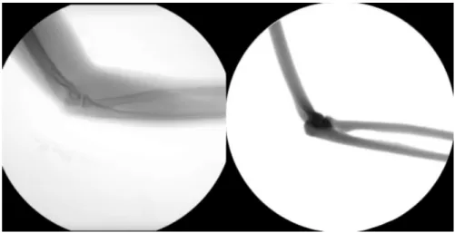
Figure 2.5: Comparison between real elbow fluoroscopic image (left panel) and the relevant Digitally Reconstructed Radiography (DRR) (right panel).
Other uniform maps with a resolution of 0.5mm were computed in order to code the space inside and outside the model with boolean values. DRRs were represented by 1024x1024 pixel wide DICOM image with pixel spacing equal to 0.37mm. The X-rays sources was virtually placed in the middle of the image at a distance of 1300mm. Initially all the pixels were set to white. Then, the models were placed in known positions and orientations in the space. For each point inside the models, a projection ray from the camera was traced and the nearest 9 pixels to point of intersection in the image were attenuated according to the Lambert-Beer law1.1. A low pass Gaussian filter was applied to smoothen the edges. Models of the calibration grid and cage were also created and the relative
2.3In-silico evaluation of the distortion correction in 3DF 45
DRRs created. A forearm flexion movement was simulated and 6 different images generated. The same images were then reprocessed to generate a second dataset considering also the simulation of geometric pincushion and sigmoidal distortion according to Fantozzi [61]. The images were then analyzed for the reconstruction of the two kinematics and the results were compared. Given the fact that the pixel spacing was estimated together with the correction of the distortion, analyzing the undistorted dataset, which do not need the correction, the pixel spacing was manually imposed to 0.37mm.
Distortion Correction and Calibration
In order to obtain a reliable representation of the fluoroscope with a perspective projection model, geometric image distortion must be taken in consideration [61] and the position in the space of the camera must be identified with high accuracy. The geometric distortion has two main sources: (a) the “pincushion effect” caused by the projection of the x-ray beam onto the curved input surface of theXRII
and (b) the deflection of the electrons inside the XRII caused by any external magnetic field producing the typical sigmoidal distortion. For image distortion correction a global warping techniques proposed by Gronenshild [60] based on a 5th degree polynomial function was used. A 2D model of a rectangular grid of tin-leaded alloy balls 5mmapart was developed and the relevant distortedDRR
was generated in order to calculate the parameters necessary for the correction. Positions of markers on the distorted image were detected. Transformations between detected and known positions of markers were then used to correct every generatedDRR image. This automatic procedure leaded also to the estimation of the pixel spacing. Another DRR was generated projecting a model of the 3D calibration cage of plexiglas containing 18 tin-leaded alloy in known position typically used for the calibration. The position of the camera was then estimated minimizing the Euclidean distance between the projection of a model of the cage and the positions of the markers center in the distortion corrected fluoroscopic image with a Nelder-Mead minimization algorithm [79].
Pose estimation
After the geometric distortion correction, a Canny’s edge detector [70] was applied to extract the bone contours. However, bones overlapping and pixel-wise noise caused the extraction of spurious contours which had to be detected and manually
erased by the operator. The method described in Section1.3.1 was applied to the distorted and to the un-distorted datasets. The minimization was carried out by applying theLMA[73].
2.3.3
Results
Undistorted dataset The DRR of the calibration cage was generated and analyzed. The principal point position of the camera (projection of the pinhole camera to the image plane) was estimated with an error minor than 0.1µmwhile the camera distance was estimated as 1299.15 mm. The poses of the forearm and of the humerus were estimated and the absolute residual deviations from the imposed kinematic were quantified. In Table 2.2 the mean (m), the standard deviation (std), the median (med) and the maximum (max) values over the six frames analyzed are reported.
Distorted dataset The pixel spacing estimated during the correction of the distortion was equal to 0.3708 mm. Analyzing the cage the camera principal point was estimated with an error minor than 0.1 µmwhile the camera distance was estimated at 1302.62mm. Results are reported in Table2.2.
2.3.4
Discussion and conclusions
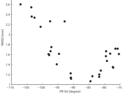
Even if the number of alignments was limited, results showed that the error was normally distributed: the information of the mean and the median values were similar. Both the alignments of the forearm and of the humerus showed the same errors. Considering the resolution of the distance maps and the error related to the contour extraction as the only sources of error, an error of about 1 mm is made for the forearm translation in x and y direction. As showed in previous works [3] the more critical pose component in mono-planar 3DFis the translation along the projection axis z, because the contour extracted from the image is not so sensitive to displacement in this direction due to the high distance of the camera. Probably better results will be achieved placing the X-ray source closer to image plane, but further investigations are needed. Regarding the rotation angles, high accuracy was achieved for the flexion-extension angle due to high sensitivity associated to lateral view, while it is possible to observe an higher variability for the other two angles that seems to be coupled with the error made for the translation along thez-axis. Comparing the data of the
2.3In-silico evaluation of the distortion correction in 3DF 47
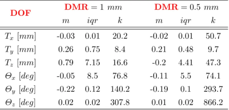
Table 2.2: Forearm and humerus residual pose deviation in terms of translation and rotation after the alignment for undistorted dataset, and after the correction of distorted images.
Forearm No Distortion Geometric Distortion
m std med max m std med max Tx [mm] 0.34 0.25 0.31 0.68 0.44 0.39 0.39 1.11 Ty [mm] 1.12 0.30 1.03 1.57 1.47 0.30 1.36 1.97 Tz [mm] 2.17 0.68 2.44 2.89 4.05 1.90 3.42 7.31 Θx[deg] 0.97 0.50 0.99 1.45 2.54 0.27 2.56 2.97 Θy [deg] 2.80 0.79 2.64 3.94 0.82 0.63 0.83 1.74 Θz [deg] 0.07 0.06 0.06 0.17 0.12 0.05 0.12 0.16
Humerus No Distortion Geometric Distortion
m std med max m std med max Tx [mm] 0.20 0.23 0.16 0.48 0.76 0.65 0.67 1.89 Ty [mm] 0.32 0.14 0.33 0.48 0.26 0.14 0.24 0.49 Tz [mm] 1.38 1.31 1.42 2.53 2.06 0.66 2.19 2.99 Θx[deg] 1.60 0.95 1.91 2.32 2.01 2.50 1.31 6.94 Θy [deg] 1.74 0.96 1.69 2.92 1.79 1.03 2.06 2.96 Θz [deg] 0.14 0.06 0.16 0.21 0.18 0.23 0.12 0.65
alignments with or without the distortion correction, the Gronenshild algorithm [60] resulted effective: there was no significant difference between the errors in the two groups of data. However, the maximum error related to theΘxangle for the
humerus is about 7 degrees. This suggest that relative minima can compromise the non-linear minimization algorithm. Before characterizing the technique in
in-vitro conditions, further study are needed to investigate how to reduce the error associated toz-axis translation and to analyze how the proposed method behave in the analysis of other motor tasks such as intra-extra rotation and at different degrees of abduction.