EFFICIENT LEARNING WITH SOFT LABEL
INFORMATION AND MULTIPLE ANNOTATORS
by
Quang Nguyen
BS, Moscow State University, 2006
Submitted to the Graduate Faculty of
the Dietrich School of Arts and Sciences in partial fulfillment
of the requirements for the degree of
Doctor of Philosophy
University of Pittsburgh
2014
UNIVERSITY OF PITTSBURGH COMPUTER SCIENCE DEPARTMENT
This dissertation was presented by
Quang Nguyen
It was defended on March 24th, 2014 and approved by
Milos Hauskrecht, PhD, Associate Professor, Computer Science
Janyce Wiebe, PhD, Professor, Computer Science
Jingtao Wang, PhD, Assistant Professor, Computer Science
Gregory Cooper, MD, PhD, Professor, Biomedical Informatics
Copyright © byQuang Nguyen
EFFICIENT LEARNING WITH SOFT LABEL INFORMATION AND MULTIPLE ANNOTATORS
Quang Nguyen, PhD
University of Pittsburgh, 2014
Nowadays, large real-world data sets are collected in science, engineering, health care and other fields. These data provide us with a great resource for building automated learn-ing systems. However, for many machine learnlearn-ing applications, data need to be annotated (labelled) by human before they can be used for learning. Unfortunately, the annotation pro-cess by a human expert is often very time-consuming and costly. As the result, the amount of labeled training data instances to learn from may be limited, which in turn influences the learning process and the quality of learned models. In this thesis, we investigate ways of improving the learning process in supervised classification settings in which labels are provided by human annotators. First, we study and propose a new classification learning framework, that learns, in addition to binary class label information, also from soft-label information reflecting the certainty or belief in the class label. We propose multiple meth-ods, based on regression, max-margin and ranking methodologies, that use the soft label information in order to learn better classifiers with smaller training data and hence smaller annotation effort. We also study our soft-label approach when examples to be labeled next are selected online using active learning. Second, we study ways of distributing the anno-tation effort among multiple experts. We develop a new multiple-annotator learning frame-work that explicitly models and embraces annotator differences and biases in order to learn a consensus and annotator specific models. We demonstrate the benefits and advantages of our frameworks on both UCI data sets and our real-world clinical data extracted from Electronic Health Records.
TABLE OF CONTENTS
1.0 INTRODUCTION. . . 1
1.1 Learning with auxiliary soft-label information . . . 2
1.2 Learning with multiple annotators . . . 4
1.3 Organization of the thesis. . . 5
2.0 BACKGROUND . . . 7
2.1 Supervised classification learning . . . 7
2.1.1 Logistic regression . . . 8
2.1.1.1 Learning the logistic regression model . . . 9
2.1.1.2 Regularization . . . 11
2.1.2 Maximum Margin method . . . 11
2.1.2.1 Linear Support Vector Machines. . . 12
2.1.2.2 Kernel Support Vector Machines . . . 14
2.2 Related work for label efficient learning . . . 16
2.2.1 Active learning . . . 17
2.2.2 Transfer learning . . . 20
2.2.2.1 Core concepts . . . 20
2.2.2.2 Types of information to be transferred . . . 21
2.2.2.3 Multitask learning . . . 22
2.2.3 Learning with auxiliary soft labels . . . 24
2.2.4 Learning with multiple annotators . . . 25
2.2.4.1 Learning the "true" label. . . 27
3.0 LEARNING WITH AUXILIARY SOFT-LABEL INFORMATION . . . 32
3.1 Introduction . . . 32
3.2 Algorithms for learning with probabilistic soft-labels . . . 35
3.2.1 Discriminative regression methods . . . 35
3.2.1.1 Linear regression . . . 35
3.2.1.2 Consistency with probabilistic assessment. . . 36
3.2.1.3 Soft-labels help to learn better classification models . . . 36
3.2.2 Noise in subjective estimates . . . 37
3.2.3 A ranking method to improve the noise tolerance . . . 39
3.2.4 Ranking methods with reduced number of constraints . . . 42
3.2.4.1 A ranking method with discrete bins of examples . . . 42
3.2.4.2 A ranking method with linear number of constraints . . . 43
3.3 Learning with auxiliary categorical soft-labels . . . 45
3.4 Experiments with UCI data sets. . . 46
3.4.1 Experimental set-up . . . 46
3.4.2 Effect of the training data size on the model quality . . . 47
3.4.3 Effect of noise on the auxiliary soft-label information . . . 49
3.4.4 Effect of the training size on the training time . . . 50
3.4.5 Effect of auxiliary soft-label information when learning with unbal-anced data sets . . . 52
3.5 Experiments with clinical data. . . 56
3.5.1 HIT and HIT data set . . . 56
3.5.1.1 HIT . . . 56
3.5.1.2 HIT data . . . 56
3.5.1.3 Temporal feature extraction . . . 57
3.5.1.4 HIT data assessment . . . 58
3.5.2 Experimental setup . . . 60
3.5.3 Results and discussion. . . 61
3.5.3.1 Experiment 1: learning with probabilistic soft-labels . . . 61
3.6 Active learning with soft-label information . . . 66
3.6.1 A query strategy for active learning with soft-label information . . . . 67
3.6.1.1 Description of the query strategy . . . 68
3.6.2 Experiments . . . 70
3.6.2.1 Experiments on UCI data sets . . . 71
3.6.2.2 Experiments on HIT data set. . . 73
3.7 Summary . . . 73
4.0 LEARNING WITH MULTIPLE ANNOTATORS . . . 77
4.1 Introduction . . . 77
4.2 Formal problem description . . . 80
4.3 Methodology. . . 81
4.3.1 Multiple Experts Support Vector Machines (ME-SVM) . . . 82
4.3.2 Optimization . . . 86
4.4 Experiments. . . 88
4.4.1 Methods . . . 88
4.4.2 Experiments on public medical data sets: Breast Cancer and Parkinsons 89 4.4.2.1 Effect of the number of reviewers . . . 90
4.4.2.2 Effect of different levels of expertise (model-consistency) . . . 91
4.4.2.3 Effect of different levels of self-consistency . . . 91
4.4.3 Experiments on HIT data set . . . 92
4.4.3.1 HIT data assessment . . . 92
4.4.3.2 Experiment: learning consensus model. . . 94
4.4.3.3 Experiment: running time for learning the consensus model . 95 4.4.3.4 Experiment: modeling individual experts . . . 97
4.4.3.5 Experiment: self-consistency and consensus-consistency . . . 99
4.5 Summary . . . 101
5.0 CONCLUSIONS. . . 103
5.1 Contributions . . . 103
5.2 Open questions . . . 105
A.1 Features used for constructing the predictive models . . . 108
A.2 Statistics of agreement between experts . . . 109
A.3 AUC and significance test results for learning with auxiliary information experiments . . . 111
A.4 Derivation of Equation 4.4 . . . 115
LIST OF TABLES
1 UCI data sets used in the experiments . . . 47
2 Basic statistics for the auxiliary soft label information collected from the ex-perts. Each expert labels 377 patient instances. The second and third columns show the distribution of probabilities for positive and negative examples. The remaining columns show the counts of strong and weak subcategories for pos-itive and negative examples. . . 59
3 Methods used in experiments with probabilistic soft-labels (experiment 1) and ordinal categorical soft-labels (experiment 2). Note: in the "Labels used" col-umn, "prob" and "categ" mean probabilistic and categorical soft-labels, respec-tively. . . 61
4 Methods for the experiments of learning with soft-labels in active learning setting. . . 71
5 AUC of different methods on medical data sets with 3 reviewers . . . 90
6 Features used for constructing the predictive models. The features were ex-tracted from time series data in electronic health records using methods from [Hauskrecht et al., 2010, Valko and Hauskrecht, 2010, Hauskrecht et al., 2013] 108
7 Expert 1 versus Expert 2, binary labels. Absolute agreement = 0.85, Kappa = 0.53 . . . 109
8 Expert 1 versus Expert 2, ordinal categorical labels. Absolute agreement = 0.61, Kappa = 0.39, Weighted Kappa = 0.47 . . . 109
9 Expert 1 versus Expert 3, binary labels. Absolute agreement = 0.84, Kappa = 0.57 . . . 110
10 Expert 1 versus Expert 3, ordinal categorical labels. Absolute agreement =
0.60, Kappa = 0.40, Weighted Kappa = 0.51 . . . 110
11 Expert 2 versus Expert 3, binary labels. Absolute agreement = 0.77, Kappa = 0.33 . . . 110
12 Expert 2 versus Expert 3, ordinal categorical labels. Absolute agreement = 0.55, Kappa = 0.26, Weighted Kappa = 0.34 . . . 110
13 All three experts, binary labels. Fleiss’ Kappa = 0.47. . . 111
14 All three experts, ordinal categorical labels. Fleiss’ Kappa = 0.34. . . 111
15 Expert 1 (figure 20(a)) . . . 112
16 Expert 2 (figure 20(b)) . . . 112
17 Expert 3 (figure 20(c)) . . . 113
18 Expert 1 (figure 22(a)) . . . 113
19 Expert 2 (figure 22(b)) . . . 114
LIST OF FIGURES
1 Discriminant functions and decision boundary. . . 9
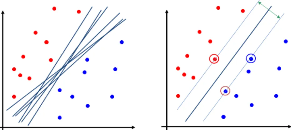
2 Maximum Margin (Support Vector Machines) idea. Left: many possible deci-sions; Right: maximum margin decision. . . 12
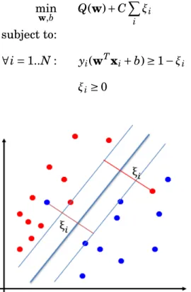
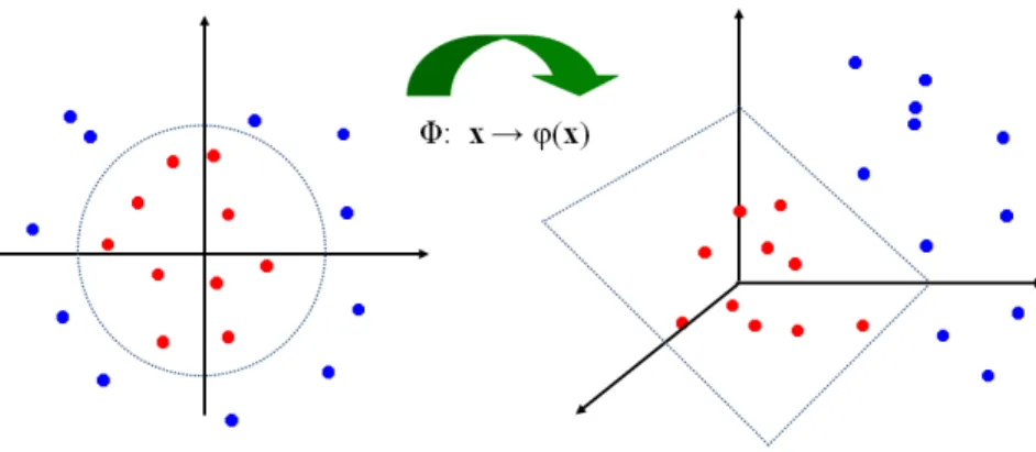
3 Soft-Margin SVM for the linearly non-separable case. Slack variables ξi rep-resent distances between examplesxi and margin hyper-planes. . . 13 4 Kernel SVM idea. Left: original 2-d input space, positive and negative
exam-ples are not linearly separable; Right: functionϕmapping original input space to a higher-dimensional (3-d) feature space, where positive and negatives can be linearly separable.. . . 14
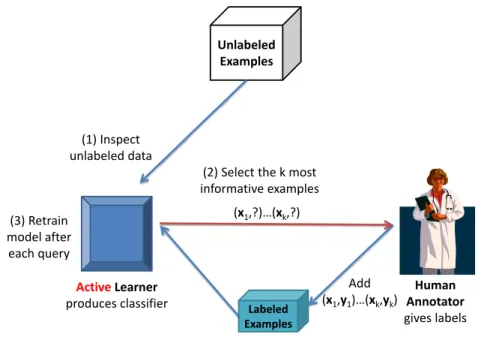
5 Active Learning scheme.. . . 18
6 Graphical model for the majority vote method. N examples labeled by K an-notators. . . 26
7 Graphical model for Dawid method [Dawid and Skene, 1979]. N examples labeled by K annotators.. . . 28
8 Graphical model for Welinder’s method [Welinder et al., 2010]. N examples labeled by K annotators.. . . 29
9 Graphical model for Raykar’s method [Raykar et al., 2010]. N examples la-beled byK annotators. . . 29
10 Regression methods LinRaux and LogRaux, that learn from probabilistic soft-label information, outperform binary classification models SVM and logistic regression (LogR), that learn from binary class labels only. The soft-labels are not corrupted by noise. . . 37
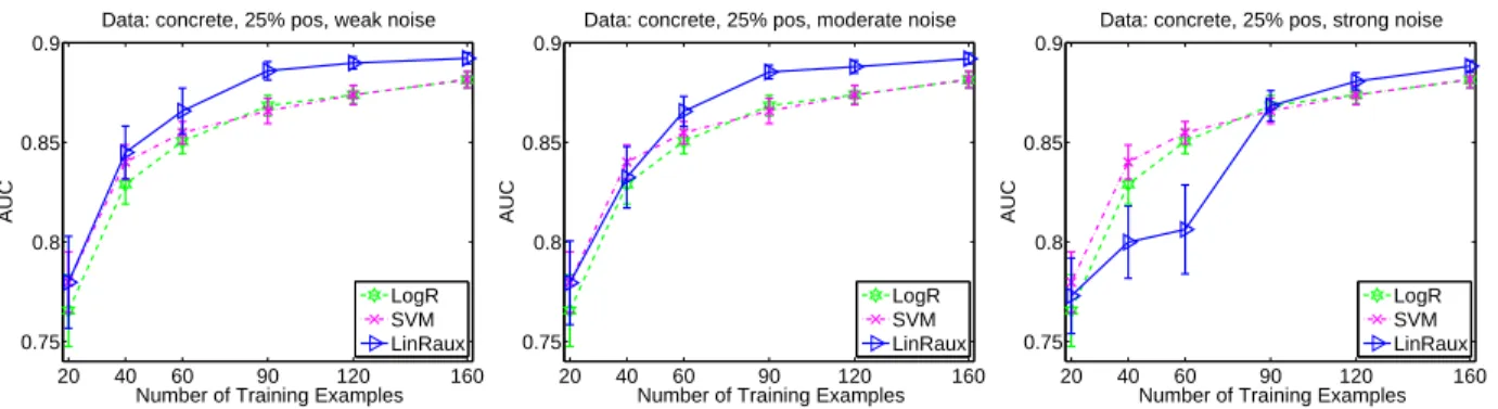
11 AUC of different models when the auxiliary soft-labels have three different lev-els of noise: (Left) weak noise, (Middle) Moderate noise, (Right) Strong noise. Regression method LinRaux clearly outperforms standard binary classifiers SVM and LogR when noise is weak. However, it’s performance deteriorates quickly as the noise increases, and is outperformed by SVM and LogR when the noise is strong. . . 38
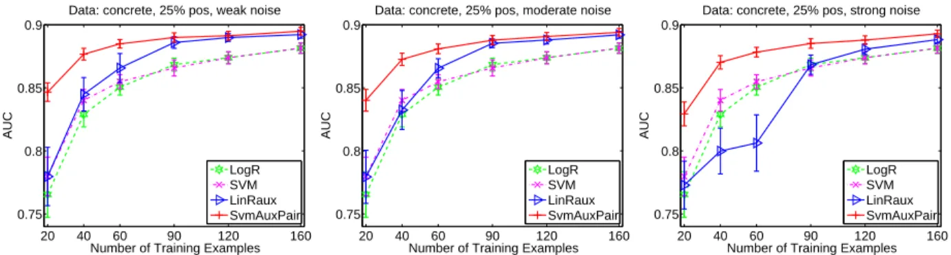
12 AUC of different models when the auxiliary soft-labels have three different levels of noise: (Left) weak noise, (Middle) Moderate noise, (Right) Strong noise. Ranking method SvmAuxPair is robust to noise and outperforms all other methods across different noise levels. . . 42
13 Ranking based on discrete bins. Examples are distributed to different bins based on their soft-labels. Optimization constraints are defined for examples and their relative positions to bin boundaries. Red and blue data points denote negative and positive examples, respectively. . . 43
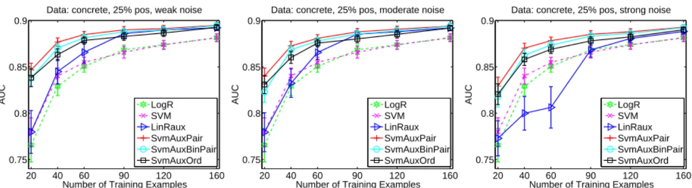
14 Ranking method SvmAuxOrd, with a linear number of optimization constraints, is robust to soft-label noise and is comparable with SvmAuxPair and SvmAuxBin-Pair, which have a quadratic number of constraints. . . 45
15 The benefit of learning with auxiliary probabilistic information on five ent UCI data sets. The quality of resulting classification models for differ-ent training sample sizes is shown in terms of the Area under the ROC curve statistic. . . 48
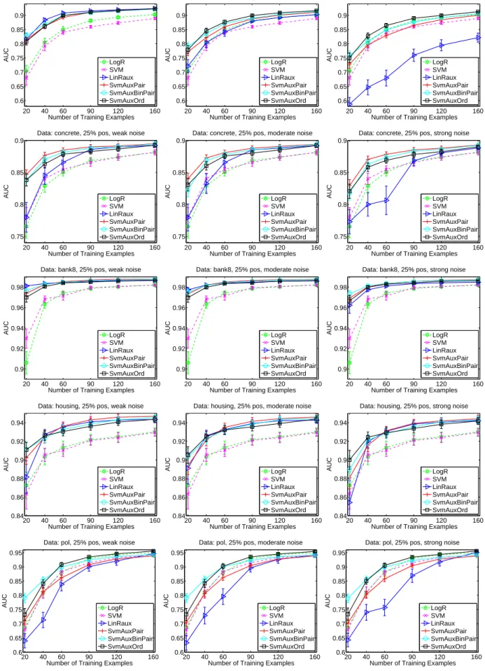
16 Learning with noise in soft-labels. AUC vs. sample size for different learning methods trained on data with soft-label information corrupted by three levels of noise: left column weak noise (5%), middle moderate noise (15%), right -strong noise (30%). One row of figures for each data set. . . 51
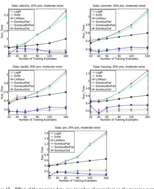
17 Effect of the training data size (number of examples) on the training running time (seconds).. . . 53
18 Learning with unbalanced data. Area under the ROC curve vs. sample size for different learning methods trained on data with different ratios of positive examples: left column - 5%, middle - 25%, right - 50%. One row of figures for each data set. . . 55
19 The figure illustrates a subset of 10 temporal features used for mapping time-series for numerical lab tests.. . . 58
20 AUC for the different learning methods trained on probabilistic soft labels from three different experts and for the different training sample sizes. . . 62
21 Distribution of probabilities assigned to negative (left) and positive (right) ex-amples by experts 1, 2 and 3, respectively. Left and right vertical bars show mean and standard deviation of assigned probabilities to negative and positive examples, respectively. The ’Overlap Region’ between horizontal dash lines is where probability estimates for positive and negative examples overlap. These inconsistencies may lead to deterioration of models trained based on such prob-abilities. . . 64
22 AUC for the different learning methods trained on ordinal categorical labels from three different experts and for the different training sample sizes. . . 65
23 The query strategy (SLDiscr) that uses soft-label information. The black points are labeled examples. The x-coordinate represents the probability of the ex-ample as estimated by the current model, while the y-coordinate shows the probability that is assigned to it by a human. . . 70
24 AUC vs. sample size for different learning methods and query strategies trained on data with auxiliary soft-label information corrupted by three levels of noise: left column - weak noise (5%), middle - moderate noise (15%), right - strong noise (30%). One row of figures for each data set. . . 72
25 AUC for different learning methods and query strategies trained on probabilis-tic soft labels from three different experts and for different training sample sizes. 75
26 AUC for different learning methods and query strategies trained on ordinal categorical labels from three different experts and for different training sample sizes. . . 76
27 The consensus model and its relation to individual expert models. . . 79
28 The experts’ specific linear models wk are generated from the consensus lin-ear model u. The circles show instances that are mislabeled with respect to individual expert’s models and are used to define the model self consistency. . 81
29 Graphical representation of the auxiliary probabilistic model that is related to our objective function. The circles in the graph represent random variables. Shaded circles are observed variables, regular (unshaded) circles denote hid-den (or unobserved) random variables. The rectangles hid-denote plates that rep-resent structure replications, that is, there are k different expert models wk, and each is used to generate labels for Nk examples. Parameters not enclosed in circles (e.g. η) denote the hyperparameters of the model. . . 83
30 UCI data: effect of number of reviewers . . . 91
31 UCI data: effect of model noise . . . 92
32 UCI data: effect of flipping noise . . . 93
33 Effect of the number of training examples on the quality of the model when: (Left) every example is labeled by just one expert; (Right) every example is labeled by all three experts . . . 95
34 Number of training examples versus running time required for learning the consensus model (in seconds).. . . 97
35 Learning of expert-specific models. The figure shows the results for three ex-pert specific models generated by the ME-SVM and the standard SVM meth-ods, and compares them to models generated by the Majority* and Raykar* methods. First line: different examples are given to different experts; Second line: the same examples are given to all experts. . . 99
36 (left top) Agreement of experts with labels given by the senior expert; (right top) Learned self consistency parameters for Experts 1-3; (left bottom) Learned consensus consistency parameters for Experts 1-3; (right bottom) Cumulative self and consensus consistencies for Expert 1-3. . . 101
PREFACE
I would like to thank everybody who made my journey to Ph.D. possible and enjoyable. First of all, I want to express my deepest gratitude to my advisor, professor Milos Hauskrecht, who has always supported me in both professional career and personal life. Milos taught me machine learning and data mining, and how to conduct high quality re-search in these fields. He also encouraged and guided me through difficult moments during my graduate school years in Pittsburgh.
I would like to thank my thesis committee, Dr. Gregory Cooper, Dr. Janyce Wiebe and Dr. Jingtao Wang, for their valuable feedback and discussions on my thesis research.
Parts of this thesis are the results of collaboration with colleagues from University of Pittsburgh. In particular, I want to thank our former post-doc, Dr. Hamed Valizadegan (currently at NASA research), who worked with me on several papers and gave me insights in many machine learning and optimization techniques. I also would like to thank Dr. Gregory Cooper, Dr. Shyam Visweswaran and former and current members of Milos’s lab: Charmgil Hong, Zitao Liu, Mahdi Pakdaman, Eric Heim, Dr. Iyad Batal (currently at GE research), Dr. Saeed Amizadeh (Yahoo Labs), Dr. Michal Valko (INRIA France), Dr. Tomas Singliar (Amazon Research) and Dr. Richard Pelikan (USC).
I am grateful to have many good friends in Pittsburgh, who made my life more enjoyable. In particular, I want to mention my best friend Nguyen Bach, who was always willing to help and gave me a lot of useful advices.
Finally, I am very grateful to my parents Le and Hung, my brother Vinh, my sister in law Hang and my niece Ha for their unlimited love, encouragement and support.
1.0 INTRODUCTION
Nowadays, large real-world data sets are collected in various areas of science, engineering, economy, health care and other fields. These data sets provide us with a great opportunity to understand the behavior of complex natural and man-made systems and their combina-tions. However, many of these real-world data sets are not perfect and come with missing information we currently have no means to collect automatically. One type of such infor-mation is subjective labels provided by human annotators in the field that assigns data examples to one of the classes of interest. Take for example a patient health record, while some of the data (such as lab tests, medications given) are archived and collected, diagnoses of some conditions, or adverse events that occurred during the hospitalization are not. In the context of supervised learning, in order to analyze these conditions and predict them, in-dividual patient examples must be first labeled by an expert or a group of experts. Moreover, supervised learning systems often perform well only if they are trained on a large number (hundreds, even thousands) of labeled examples. However, the process of labeling examples using subjective human assessments faces a number of problems:
First, collecting labels from human annotators can be extremely time-consuming and costly, especially in the domains where data assessment requires a high level of expertise. For example, in our disease diagnostics task, an experienced physician needs to spend about
five minutes (on average) to review and evaluate one patient case [Nguyen et al., 2011a];
or in speech recognition tasks, [Zhu, 2005] reports that a trained linguist may take up to
seven hours to annotate one minute of audio record (e.g. 400 times as long). The challenge is to find ways to reduce the number of examples that need to be reviewed and labeled by an expert while improving the quality of the models learned from these examples.
it is hard to expect that one annotator/expert will be able to label all examples. To address this, instead of using one annotator, we can use multiple annotators to label examples. However, different annotators may have different opinions, knowledge or biases, which lead to disagreements in the labeling. For example, one physician may diagnose a patient as having a certain disease, while another may say the opposite. Modelling and combining all agreements/disagreements among annotators is an important and interesting problem. Studying of this problem would help us get more insights into the labeling process, improve the quality of labels and the performance of learning models.
The first problem focuses more on the quantityof labels, while the second one focuses
more on the quality of labels. In this thesis, we study and develop approaches to address
both quantity and quality aspects of the annotation and learning process. Our ultimate goal is to increase the performance of classification models, while reducing and distributing the cost of labeling. Note that our work was originally motivated by applications in medical do-main, so many examples and discussions in this thesis are related to this domain. However, in general, our proposed methods can be successfully applied in other domains, as we will demonstrate on many real-world benchmark data sets.
1.1 LEARNING WITH AUXILIARY SOFT-LABEL INFORMATION
The problem of optimizing the time and cost of labeling has been studied extensively in ma-chine learning research community. One of the most popular research directions for this
problem is Active Learning [Cohn et al., 1996]. The goal of active learning research is to
develop methods that analyze unlabeled examples, prioritize them and select those that are most critical for the task we want to solve, while optimizing the overall data labeling cost. We explore another direction that is orthogonal to the active learning approach, which can help us to alleviate the costly labeling process in practice. The idea is based on a simple premise: a human expert who gives us a subjective label can often provide us with auxiliary information, which reflects his/her certainty in the label decision, at a cost that is insignifi-cant when compared to the cost of example review and label assessment. To illustrate this
point, assume an expert reviewing electronic health record (EHR) data in order to provide some diagnostic assessment of the patient case. The complexity of clinical data prompts him/her to spend a large amount of time reviewing and analyzing the case. However, once the example is understood and the label decision is made, the cost of providing additional assessment of the confidence in this decision is relatively small. For example, according to our studies analyzing adverse clinical events (Heparin Induced Thrombocytopenia and Amiodarone Toxicity), experts spend four to six minutes before they make a decision on the condition and whether it is worthwhile to alert on it. In contrast, it takes them only a few seconds to provide an auxiliary assessment of confidence, e.g. the probability of having dis-ease or the strength of the alert. Clearly, the cost to obtain this auxiliary information is insignificant compared to the whole data acquisition cost. The question is how to utilize it efficiently?
We propose and study a machine learning framework in which a classification learning problem relies, instead on just the binary class label information, on a more refined soft-label information reflecting the certainty or belief in this soft-label. In general, this information can be a probabilistic/numeric score, e.g. chance of having disease is 0.7/1, 7/10, etc. or a qualitative category, e.g. weak, medium, strong belief in having disease. We expect this auxiliary soft-label information, when properly used, can help us to learn a better classifica-tion model. Briefly, we expect an instance with a high (or low) probability should be easier to classify by a proposed machine learning model, while an instance with probability close to 0.5 likely indicates the instance is harder to classify and is close to the decision bound-ary. The limitation of soft labeling is that assessments may be subject to noise. Studies by [Suantak et al., 1996,Griffin and Tversky, 1992,O’Hagan et al., 2007] showed that hu-mans are not very good in assigning subjective probabilities. To address the problem, we propose novel methods based on the support vector machine and learning to rank method-ologies, that are more robust to noise and able to learn high quality classifiers with smaller numbers of examples.
Note that our learning from auxiliary soft labels approach is complementary to active learning: while the later aims to select the most informative examples, we aim to gain more useful information from those selected. This gives us an opportunity to combine these two
approaches.
1.2 LEARNING WITH MULTIPLE ANNOTATORS
In practice the labeling process is often tedious and time consuming. At the same time the human expert effort is scarce. Therefore, it is hard to expect that one annotator/expert will be able to label all examples. To address this problem, we investigate and develop a learning framework that lets us use the labels obtained from multiple expert annotators. Our objective is to build a "consensus" model that agrees as much as possible with all experts and generalizes well on future unseen data. Note that this setting is different than the traditional supervised learning: instead of having a single annotator, we have a group of annotators labeling examples.
The biggest challenge in multiple-annotator learning is how to model and combine all agreements and disagreements among annotators. To develop a consensus model, we need to grasp the causes for the labeling disagreement of different annotators. The labeling dis-agreement may be rooted in (1) differences in the risks annotators associate with each class label assignment, (2) differences in the knowledge (or model) annotators use to label exam-ples, and (3) differences in the amount of effort annotators spend for labeling each case. To illustrate the nature of these differences, let us consider the problem of diagnosing a patient from noisy and incomplete observations. First, diagnosing a patient as not having a disease when the patient has disease, carries a cost due to, for example, a missed opportunity to treat the patient, or longer patient discomfort and suffering. A similar, but different cost is caused by incorrectly diagnosing a patient. The differences in the annotator-specific utilities (or costs) may explain differences in their label assessments. Second, while diagnoses pro-vided by different experts may be often consistent, the knowledge they have and features they consider when making the disease decision may differ, potentially leading to differ-ences in labeling. It is not rare when two expert physicians disagree on a complex patient case due to differences in their knowledge and understanding of the disease. These differ-ences are best characterized as differdiffer-ences in the model they use to diagnose the patient.
Third, different experts may spend different amounts of time to review the case and decide on the diagnosis. This may lead to mistakes in the labeling that are inconsistent with the expert’s own knowledge and model. Our objective is to develop a learning framework that will embrace these types of differences and find a consensus model.
In this dissertation, I propose and develop a new multiple-annotator learning approach that takes into account the annotators’ reliability as well as differences in the annotator-specific models and biases when learning a consensus model.
1.3 ORGANIZATION OF THE THESIS
This thesis is organized as follows:
Chapter 2 provides background and relevant research for supervised classification and
approaches for label efficient learning. In particular, we start with an overview of super-vised classification learning, with more details on logistic regression and maximum margin methods. Then we review relevant research in active learning, transfer learning, learning with auxiliary soft-label information and multi-annotator learning fields.
Chapter3describes our approach for learning with auxiliary soft-label information and
the combination of active learning and auxiliary information in one learning framework. We demonstrate the benefits of our methods on a number of UCI data sets, while adding noise to auxiliary assessments. We also test our approach on real medical data representing
experts assessment of the risk of the Heparin Induced Thrombocytopenia (HIT) [Warkentin
et al., 2000] given a set of patients’ observations and labs.
Chapter 4 describes our approach for learning with multiple annotators, followed by
experimental results. We study our framework on synthetic (UCI-derived) datasets and on our real-world multiple expert learning problem in medical domain. First, for the synthetic data we start from the ground consensus model and show that we can recover it accurately from simulated experts’ labels that may differ because of the expert-specific parameters. Second, we show benefits of our approach on HIT data.
Finally, I would like to note that parts of this thesis have been previously published in [Nguyen et al., 2011a], [Nguyen et al., 2011b], [Nguyen et al., 2013], [Valizadegan et al., 2012], [Valizadegan et al., 2013].
2.0 BACKGROUND
This chapter outlines background and relevant research for methods we describe in this thesis. We start with the basics of supervised learning and classification methods, then discuss label efficient learning and related works. We use the following notation throughout this document: matrices are denoted by capital letters, vectors by boldface lower case letters and scalars by normal lower case letters.
2.1 SUPERVISED CLASSIFICATION LEARNING
Supervised learning is a sub-field of machine learning, where the task is to learn a mapping from input examples to desired output targets. In the standard supervised setting, training data consist of examples and corresponding labels (targets), which are given by a teacher (labeller). The goal is to learn a model that can accurately predict labels of future unseen examples. Formally, given training data D={d1,d2, ...,dN} where di is a pair of (xi,yi), xi
is an input feature vector, yi is a desired output given by a teacher, the objective is to learn a mapping function f :X→Y such that for a new future examplexnew, f(xnew)≈ ynew. If
desired outputs are continuous values then the learning problem isregression, otherwise
the learning problem isclassificationif desired outputs are discrete.
In this thesis we focus on the classification learning, which has many applications in practice, for example, given historical clinical data, predict whether a (future) patient has disease or not, or given a text database, classify a new text document to one of possible topics (news, sport, etc.). In general, there may be any number of desired class outputs, however, the most frequently researched problem is binary classification, where outputs belong to
two classes, e.g. a disease is detected/not detected.
The exact form of the model f :X →Y, and the algorithms used to learn it, can take
on different forms. For example, the model can be based on linear discriminant analysis
(LDA) [Fisher, 1936], logistic regression [McCullagh and Nelder, 1989], maximum margin
(support vector machines) [Cortes and Vapnik, 1995], probabilistic models such a Naive
Bayes model [Domingos and Pazzani, 1997] or a Bayesian belief network [Pearl, 1985], and
classification trees [Breiman et al., 1984]. In addition, there are various ensemble methods,
such as bagging [Breiman, 1996] and boosting [Schapire, 1990], where multiple individual
(weak) learners are combined together to create a strong one.
In this chapter, we describe Logistic Regression [McCullagh and Nelder, 1989] and
Max-imum Margin [Cortes and Vapnik, 1995] methods in more details. These are the two of the
most widely used baselines in classification learning research. Moreover, many methods mentioned in this thesis, including some of ours, are based on these methods, so a review of them would be useful.
2.1.1 Logistic regression
We want to learn a classification function f :X →Y, that maps input (features) X to one
of the class labels {0, 1..k} inY. One way to do this is to define a function gi(x) :X→R for
each class i∈{0, 1, ..,k}, then classify an input examplexto the class with the highest value of gi(x), i.e. f(x)=argmaxi∈{0..k}gi(x). Intuitively, function gi(x) represents a kind of class
membership, and an example belongs to the class for which it has the highest membership value.
For illustration let us consider the binary classification case, i.e. Y ∈{0, 1}. Figure 1
illustrates the input space with positive and negative examples and the decision boundary defined by gi(x), i∈{0, 1}. If g1(x)> g0(x) then x belongs to class 1 (positive), otherwise it belongs to class 0 (negative). The decision boundary is defined when g1(x)=g0(x), e.g.
membership values are equal.
Figure 1: Discriminant functions and decision boundary.
Nelder, 1989], one of the most commonly used models, defines g1and g0as follows:
g1(x) = 1
1+e−wTx=p(y=1|x,w)
g0(x) = p(y=0|x,w)=1−p(y=1|x,w)
An examplexwill be assigned to class 1 if g1(x)≥0.5, and class 0 otherwise.
The main idea of logistic regression is to obtain a probabilistic interpretation of class
membership by transforming a linear combination of input vectorx, i.e. wTx, into a
proba-bilistic value. The logistic function 1
1+e−wTx is useful because it can take any inputw
Txfrom
(−∞,+∞) range and transforms it into an output in (0,1) range.
2.1.1.1 Learning the logistic regression model LetDi=(xi,yi) denotes the set of in-put examplesxiand labels yi, andµi=p(yi=1|xi,w)=g(wTx). We learn logistic regression
model by maximizing the likelihood of data:
w∗=argmaxwL(D,w) where L(D,w) = N Y i=1 p(y=yi|xi,w) = N Y i=1 µyii (1−µi)1−yi
This is equivalent to maximizing the log-likelihood of data since the optimal weights are the same for both likelihood and log-likelihood:
w∗ = argmaxw[logL(D,w)] (2.1) = argmaxwl(D,w) = argminw−l(D,w) = argminw−log N Y i=1 p(y=yi|xi,w) = argminw−log N Y i=1 µyii (1−µi)1−yi = argminw− N X i=1
yilogµi+(1−yi) log(1−µi)
We can solve the optimization problem maxwl(D,w)= minw−l(D,w) by taking the
derivatives and updating the weight vector w by some scheme, for example, gradient
de-scent. More specifically, the gradient of the log-likelihood of data for the logistic regression model becomes: 5w−l(D,w)= N X i=1 −xi(yi−f(w,xi))
The gradient descent procedure can be implemented by iteratively updating weights as:
w(k)=w(k−1)+α(k)
N
X
i=1
−xi(yi−f(w,xi))
wherekindicates thek-th step of the updating process andα(k) is the learning rate scaling the iterative updates.
In this section we gave a brief review of logistic regression, more details about theory
2.1.1.2 Regularization Over-fitting problem is a problem in which a learner achieves high performance on training, but poor performance on test data. It can arise when the
dimensionality ofxis high while the number of training examplesNis small. We can reduce
the over-fitting effect by using one of the regularization approaches, such as the ridge (or L2) regularization [Hoerl and Kennard, 1981], the lasso (or L1) regularization [Tibshirani,
1996,Friedman, 2010], or their elastic network combination [Zou and Hastie, 2005]. Using
regularization, the optimization in Equation2.1is modified to:
w∗=argminwLoss(D,w)+Q(w)
whereLoss(D,w)= −logL(D,w) for logistic regression andQ(w) is a regularization penalty. Examples of regularization penalties are: Q(w)=λ||w||1 =λPdj=1|wj| for the L1 (lasso)
regularization, or Q(w)=λ||w||2 =λ(Pd
j=1w 2
j)
1
2 for the L2 (ridge) regularization. λ is a
constant that scales the regularization penalty. Typically this constant is optimized using the internal cross-validation approach.
2.1.2 Maximum Margin method
The main idea of the Maximum Margin method for classification is to find the decision hyper-plane that maximizes the margin between examples of the two classes. "Margin" is defined as the distance from the closest examples to the decision hyper-plane. The intuition is that among all possible decisions, the max-margin decision has the best generalization ability. In other words, it has the best chance to classify a future example correctly. This intuition was proved to be true. In fact, the idea has a strong foundation in statistical
learning theory: [Vapnik, 1995] proved that the bound on generalization error is minimized
by maximizing the margin.
Figure 2 illustrates this idea. In Figure 2-left positive and negative examples can be
perfectly separated by many linear decision boundaries. However, as argued by [Vapnik,
1995] and [Cortes and Vapnik, 1995], the optimal solution is the decision boundary that
maximizes the margin between positive and negative examples (Figure2-right).
Note that the decision hyper-plane is determined only by the examples on the margin hyper-planes (circled points in Figure 2-right). Hence, these examples are called "support
vectors". In machine learning literature, Maximum Margin method for classification is often referred by the term "Support Vector Machines".
Figure 2: Maximum Margin (Support Vector Machines) idea. Left: many possible decisions; Right: maximum margin decision.
We briefly describe mathematical formulations of Linear SVM and Kernel SVM in the following sections.
2.1.2.1 Linear Support Vector Machines Let start with a simple case, when data are
linearly separable. Figure2illustrates a 2-d example of this case.
Linear SVM can be formulated by the following constrained optimization problem:
min
w,b Q(w)
subject to:
∀i=1..N: yi(wTxi+b)≥1
where Nis the number of examples in the training data,wis the weight vector - the model
to be learned. w defines the direction of the decision boundary. b is the bias term, which
defines the shift of the boundary. xiandyi∈{1,−1} are feature vector and label, respectively, of example i. Q(w) is a regularization function (Section2.1.1.2), which is typically written in L2 norm in machine learning literature, but in general can be in L1 norm. For classification, a new examplexis assigned "1" (positive) if (wTx+b)>0, otherwise "-1" (negative).
The above SVM formulation is called Hard-margin SVM, because it requires all exam-ples of the two classes to be linearly separable. However, in practice, it is often impossible
to separate data perfectly with a linear boundary, as shown in Figure 3. To handle this case, we relax the above requirement by allowing SVM to make mistakes, but mistakes are penalized in the objective function. We have the following formulation of Soft-margin SVM,
also called theprimal formof (Soft) SVM:
min w,b Q(w)+C X i ξi (2.2) subject to: ∀i=1..N: yi(wTxi+b)≥1−ξi ξi≥0
Figure 3: Soft-Margin SVM for the linearly non-separable case. Slack variablesξirepresent
distances between examplesxi and margin hyper-planes.
Slack variables ξi represent distances between examples xi and margin hyper-planes.
Note that ξi=0 if xi is located on the correct side of the margins, otherwise ξi >0. ξi =
max(0, 1−yi(wTxi+b)) is called the hinge loss. Constant C is a trade-off parameter that
defines how much misclassified examples should be penalized. In fact, Hard-margin SVM is a special case of Soft-margin SVM with C set to infinity. Therefore, further in this document, the term "Support Vector Machines" refers to Soft-margin SVM.
Both Hard and Soft-margin formulations are convex optimization problems, which means that any local optimum is also the global optimum. This property is very important because it indicates that if we can find a best local solution, we are guaranteed to have the best
global solution. This is not the case for many other classification methods (logistic regres-sion, neural networks, etc.), where we may be "trapped" in local optima and never find the global optimum.
2.1.2.2 Kernel Support Vector Machines Linear SVM with soft margins is a powerful tool when the non-separability is caused by a small number of (noisy) examples. However, if data are highly non-linear and are not separable by a linear boundary, e.g. data shown
in Figure 4-left, then Linear SVM may not perform well. Kernel SVM was designed to
solve this problem. The idea is to map features from the original space to a new higher dimensional space, where linear relations may exist. Figure4illustrates this idea: Figure4 -left shows positive and negative examples that cannot be separable in the 2-d space; Figure
4-right shows that mappingϕof input data from the original 2-d space to a 3-d space may
introduce a linear boundary that can separate examples of two classes (in this case the linear boundary is a surface).
Figure 4: Kernel SVM idea. Left: original 2-d input space, positive and negative examples
are not linearly separable; Right: function ϕ mapping original input space to a
higher-dimensional (3-d) feature space, where positive and negatives can be linearly separable.
Solving the optimization problem 2.2 in the feature space is equivalent to solving the
optimization of the following Lagrangian function:
min w,b L(w,b,a)= 1 2||w|| 2 − N X i=1 ai(yi(wTϕ(xi)+b)−1)
where a=(a1, ...,aN)T is the vector of Lagrangian multipliers. Note that for the
demon-stration purpose we use L2 norm regularization||w||2, which is widely used in the machine
learning literature.
Setting the derivatives of L(w,b,a) with respect tow and b equal to 0, we obtain the following two conditions:
w = N X i=1 aiyiϕ(xi) 0 = N X i=1 aiyi
Plugging these conditions into L(w,b,a) gives thedual formof the maximum margin
problem: max a1..aN N X i=1 ai− 1 2 N X i,j=1 aiajyiyjk(xi,xj) subject to: ∀i=1..N: 0≤ai≤C N X i=1 aiyi=0
wherek(xi,xj)=ϕ(x)Tϕ(x0) is a kernel function. For Linear SVM,k(xi,xj) is the dot product ofxi andxj : k(xi,xj)=xi·xj.
Solving constrained optimization problems in high dimensional spaces is difficult and
computationally expensive. Therefore, kernel functionsk should be designed so that SVM:
(1) has the representation power of high dimensional spaces and (2) still be computationally
efficient. This can be done by choosing a mapping from the input space I to a new feature
spaceF:x−→ϕ(x) , such thatk(x,x0)=ϕ(x)·ϕ(x0)∀x,x0∈I. Thus, we implicitly compute dot
product in a high dimensional spaceF, in terms of operations in the original low dimensional
space I. This is called the "kernel trick".
Many different types of kernels have been designed by the research community. For example, the two most widely used kernels are polynomial and radial basis functions (RBF):
• RBF:k(x,x0)=ex p(−||x−x0||2
2σ2 )
In this section we gave a brief review of Support Vector Machines. More details about theory
and analysis of SVM can be found in [Cortes and Vapnik, 1995] and [Bishop, 2006].
2.2 RELATED WORK FOR LABEL EFFICIENT LEARNING
By definition supervised learning systems rely on labels given in the training data, and in practice, they often must be trained on a large number of labelled examples in order to perform well. However, as mentioned in the Introduction chapter, the process of labeling examples using subjective human assessments faces two problems: (1) it can be extremely time-consuming and costly, which results in a limited number of labeled examples, and (2) in many cases labels are given by not only one but multiple annotators, which may introduce disagreements/contradictions due to differences in knowledge, opinions or biases. Since supervised learning methods rely on labeled examples, we need to find approaches to obtain more useful information (labels) with lower cost and utilize them efficiently. Again, in this thesis, we focus on classification learning, where our goal is to build classification models that can learn with smaller training data and make more accurate prediction on future unseen examples.
In this section we give an overview of research works that are relevant to our solutions
for above problems. In Section2.2.1we review active learning - a sub-field of machine
learn-ing that aims to reduce labellearn-ing cost by selectlearn-ing the most informative examples. In Section
2.2.2we review transfer learning that aims to reducing labeling cost by transferring useful information from one domain/task to another domain/task. Then we give an overview of our alternative approach - learning with auxiliary soft labels and its relevant research. In Sec-tion2.2.4we summarize works in multi-annotator learning, where the two main objectives are estimating the "true" labels and learning a consensus model, given information collected from multiple annotators.
2.2.1 Active learning
Active Learning is a sub-field of (supervised) machine learning, where the primary goal is to reduce the cost of labeling examples. Active learning has been explored extensively by the data mining and machine learning communities in recent years. In traditional "passive" learning, the learner randomly picks examples from the database and requests labels for them. In contrast, active learning only requests labels for the most informative examples -ones that help to increase the performance of the current learning model. Intuitively, this may reduce the number of examples to be labeled and accelerate the learning process.
There are two common query scenarios: stream-based [Cohn et al., 1994] and pool-based
[Lewis and Gale, 1994]. In the stream-based scenario, data come in a stream, one example at a time, the active learner set an "informativeness" threshold and decides whether to query for label or discard this example based on that threshold. In the pool-based scenario, the active learner has access to a pool (subset) of all unlabeled examples. It inspects examples in
the pool and selects the k most informative examples to query for labels. While pool-based
scenario is used much more common in practice, stream-based scenario is more appropriate in the case when limited processing power does not allow us to scan and inspect a pool of examples (e.g. mobile applications).
Figure 5 illustrates how (pool-based) active learning works. An active learner
recur-sively performs three steps: (1) inspects unlabeled examples; (2) selects the mostk
informa-tive examples and requests an annotator to label them, and (3) retrains the current learning model with the new set of labeled examples. This process is repeated until some stopping criteria is met, for example, N examples have been labeled, or the performance the model has reached some satisfied threshold.
In all the scenarios, the active learner needs to select example(s) based on some "in-formativeness" criteria. Different strategies to define the "in"in-formativeness" have been pro-posed. We summarize the most popular ones in the following paragraphs.
Uncertainty sampling [Lewis and Gale, 1994] is the simplest and most widely used query
strategy. It queries the example that the current model predicts with the lowest confidence. For binary classification, uncertainty sampling selects the example that has predictive
prob-ActiveLearner produces classifier Human Annotator gives labels Unlabeled Examples Labeled Examples (3) Retrain model after each query (1) Inspect unlabeled data
(2) Select the k most informative examples
(x1,?)…(xk,?)
Add (x1,y1)…(xk,yk)
Figure 5: Active Learning scheme.
ability closest to 0.5. The idea is intuitive: if the current model can predict an example with high confidence then this example does not carry much information to improve the model; otherwise the example can benefit the model. For regression task, the learner queries the example for which the current learning model has the highest output variance in its predic-tion (e.g. least confidence).
Another popular strategy is query-by-committee (QBC) [Seung et al., 1992]. In QBC, one
first constructs a committee of different models, which are all trained on the current labeled training data, but represent competing hypotheses. Then, committee members vote on the labeling of query candidates. The most informative example to be queried is the one that the committee members most disagree on. The construction of committee may be done in
different ways. For example, the approach introduced by [Seung et al., 1992] simply samples
randomly two hypotheses that are consistent with the current labeled training examples.
Another approach is query-by-bagging [Abe and Mamitsuka, 1998]. It repeatedly samples
subsets of labeled instances (using bagging [Breiman, 1996]) and trains committee models
on them. The size of committee may vary, however previous works have shown that even
a small committee (size two or three) could work well in practice ( [Settles, 2010], [Seung
et al., 1992], [Settles and Craven, 2008]).
change to the current model if we knew their labels. The intuition is that if an example changes the current learning model significantly then it likely carries much information and can make great impact on the learning process. One example of the expected model
change strategy is the method by [Tong and Koller, 2000], where examples are selected to
maximize the Kullback-Leibler divergence between the new posterior distribution obtained after training with the new queried label and the current posterior distribution (before the query). Another example of this query strategy is the "expected gradient length" method
introduced by [Settles et al., 2008], where the model change was defined as the Euclidean
length of the training gradient (the vector used to estimate parameter values during the optimization process). The disadvantage of the expected model change strategy is that "in-formativeness" can be over-estimated, for example, gradient may be too large if some pa-rameters become large during the optimization. Therefore, some techniques, e.g. parameter regularization, need to be used to alleviate this problem.
Expected error reduction strategy was first proposed by [Roy and McCallum,]. It aims to
directly reduce the generalization error of the learning model. The idea is that, for each
ex-amplexiin the unlabeled pool, the learning algorithm estimates its label and builds a model
over the combination of xi and the training labeled examples. Among them, the example
that minimizes the generalization error is selected to query for label. The disadvantage of this strategy is the expensive computational cost.
Variance reduction strategy [Geman et al., 1992] was originally designed for
regres-sion task, but could be generalized for classification task. This strategy queries example that would minimize the prediction variance of the current model. The intuition is that the generalization error can be indirectly reduced by minimizing output variance. To use this strategy one must have a way to approximate the output variance, which is not a triv-ial problem, and also depends on specific learning models. Closed-form approximations of
output variance were derived for Gaussian random fields [Cressie, 1993] and Neural
2.2.2 Transfer learning
Transfer learning is an emerging field in machine learning research, that aims to improve the sample complexity of learning problems with the help of additional information and knowledge sources. The main idea is to transfer useful knowledge/information learned in one domain or task (source) to another (target) domain or task. This would help to increase the amount of information that the target learner can learn form, which leads to improved predictive performance. This is not a trivial problem because we need to find out what infor-mation is useful and beneficial for the target learner, and how to transfer that inforinfor-mation.
2.2.2.1 Core concepts For the discussion of transfer learning we need to give the def-initions of the core concepts: domain, task and transfer learning. For illustration let us consider an application example: disease diagnosis, where given patient health records, the goal is to classify them into certain classes.
Domain, denoted byD, consists of two components: the feature spaceX and the marginal distributionP(X).
Task, denoted by T, consists of two components: the label space Y and a predictive
function f that maps the feature space to the label space: f :X →Y. From probabilistic
point of view, f is the conditional probability P(Y|X). The function f needs to be learned from the training data, and can be used to predict the label of a future example.
Source domainandsource taskare denoted byDS andTS, whereastarget domain
andtarget taskare denoted byDT andTT, respectively.
Transfer Learning is a learning technique that aims to improve the predictive
per-formance of the function fT in DT by using the information and knowledge inDS andTS,
whereDS6=DT and/orTS6=TT.
GivenDS,TS,DT andTT, we may have the following cases:
• The case when DS =DT and TS =TT. This is the traditional classification learning,
where we have one domain and one task.
• The case whenDS6=DT. In this case either (1) the feature spaces in source and target
bio characteristics, or (2) the feature space is the same but feature distributions are dif-ferent: P(XS)6=P(XT), e.g. patient data in source and target domains focus on different patient demographics (different countries, different age groups, etc.)
• The case when TS6=TT. In this case we have either (1) the label spaces in source and
target domains are different, e.g. there are two classes in the source domain and five classes in the target domains, or (2) the label space is the same but the label distributions are different: P(YS|XS)6=P(YT|XT), e.g. the source and the target set of patient records
have very different ratios of positive/negative examples.
• The case whenDS6=DTandTS6=TT. This is the combination of the previous two cases.
2.2.2.2 Types of information to be transferred The most important question of trans-fer learning is "What to transtrans-fer ?". According to [Pan and Yang, 2010], there can be four different types of information to be transferred from the source domain/task to the target domain/task:
• Instance transfer. The main idea of this approach is to transfer a set of labeled train-ing instances from the source data to the target data. The predictive performance is expected to increase because the target learner has acquired more labeled data to learn from. The source data usually cannot be used directly for the target task, so typically some re-weighting technique is developed to assign the weights or importance of the transferred data instances in the new domain/task. Some related works in this area are [Dai et al., 2007], [Jiang and Zhai, 2007], [Zadrozny, 2004].
• Feature representation transfer. The main idea of this approach is to utilize infor-mation from the source and target domains to learn a good feature representation that reduces the difference between these domains and decrease error rates. The predictive performance is expected to increase with the new (better) feature set. Some related
works are [Argyriou et al., 2007a], [Lee et al., 2007], [Ruckert and Kramer, 2008]. A
representative work is [Argyriou et al., 2007a], where the authors proposed to learn a
low-dimensional feature representation that is shared between source and target tasks. • Parameter transfer. The main idea of this approach is to assume that the source and target tasks have some shared parameters or prior distributions of hyper-parameters
and the approach aims to increase the performance of the target learner by exploiting
these parameters. Some related works for the parameter transfer approach are ( [
Evge-niou and Pontil, 2004], [Gao et al., 2008], [Lawrence and Platt, 2004]). In Section2.2.2.3
we will give more details about [Evgeniou and Pontil, 2004] - a representative work in
this area.
• Relation transfer. The main idea of this approach is to assume that some relations among the data in the source and target domains are similar. Therefore, the learner in the target domain can benefit by transferring these relations from the source do-main. Methods for relation transfer typically use some statistical learning technique (e.g. Markov Logic network) to transfer relation in data from the source to the target
domain. Some related works in this area are ( [Mihalkova et al., 2007], [Davis and
Domingos, 2009]). Note that data are usually in relational domains (e.g. entities are predicates and their relations are in first-order logic), and not assumed to be indepen-dent and iindepen-dentically distributed (i.i.d).
2.2.2.3 Multitask learning Multitask learning is a special type of transfer learning. The reason we have a special interest in multitask learning is that it motivated our
so-lution for the multi-annotator learning problem (Section 2.2.4 and Chapter 4). The main
differences between multitask learning and (general) transfer learning are:
• In multitask learning we have many different tasks and the domain of all tasks is the same, whereas in transfer learning the relations between tasks and between domains could be in any combination (Section2.2.2.1).
• While transfer learning focuses on improving the predictive performance of the target learner, multitask learning learns all tasks simultaneously and aims to improve the performance of all involved learners.
The main idea of multitask learning is that it assumes involving tasks are different but related, i.e. they share some related information that can help to improve the learning of all tasks simultaneously. Related works in this area aim to discover this shared information
the information among tasks through the shared hidden layer nodes in Neural Networks. [Yu et al., 2005], [Argyriou et al., 2007b], [Evgeniou and Pontil, 2004] transfer information through shared parameters of task-specific models.
A representative work in this area is [Evgeniou and Pontil, 2004], where the authors
proposed a SVM-based method for multitask learning. The idea is to separate the weight
vector w to be learned by the SVM into two components: a shared weight vector that is
common for all tasks; and a task specific weight vector, one for each task:
wt=w0+vt, t∈{1..T}
where T is the number of tasks, w0 is the shared common weight vector, wt is the weight
vector for tasktandvt is the difference betweenw0 andvt.
w0 andwt are incorporated into a single optimization problem and learned
simultane-ously during the optimization process:
min w0,vT,ξit T X t=1 m X i=1 ξit + λ1 T T X t=1 kvtk2+λ2kw0k2 s.t. ∀i∈{1, 2, ...,m} and t∈{1, 2, ...,T}: yit(w0+vt)·xit ≥ 1−ξit, ξit ≥ 0
where mis the number of training examples,ξit are slack variables that penalize
misclas-sification errors,λ1andλ2are regularization constants andxitare feature vectors.
Note that we adopt the idea of learning the common and specific tasks for solving the
multi-annotator learning problem (Section2.2.4). Our approach learns a common consensus
model and annotator-specific models simultaneously. However, we go beyond the Evgeniou and Pontil’s multitask learning approach by also incorporating the consistency and bias of different annotators into the optimization process. Details of our multi-annotator learning
2.2.3 Learning with auxiliary soft labels
We have done an overview of two popular label-efficient learning approaches: active learning and transfer learning. In this work we study an alternative approach: enrichment of labeled instances using auxiliary soft label and its incorporation into the classification learning. The idea is simple: we ask a human expert annotator to provide us, in addition to class label, also auxiliary soft label, reflecting his belief/certainty in the class label. This auxiliary information can be obtained with little extra cost because most of the time was already spent on example assessment and making class decision. Now, for each example, instead of having only class label, we have both class and soft labels. The question is how to efficiently utilize both kinds of labels to improve classification learning.
This problem is different than active learning: while active learning aims to select in-formative examples to label, we aim to obtain more useful information from those examples that are selected. This problem is also different than transfer learning because we work in the same domain, with the same data set, the auxiliary information is (always) directly relevant and available.
Since there are two kinds of labels available, this problem has close relationships to both classification, regression, and also preference learning. Previous works in the machine learning and AI community focused on one of these, but not their combination. For example, classification algorithms (e.g. logistic regression, SVM) would use only class labels. [Smyth, 1995] used probabilistic labels to learn classification of volcanoes from radar images of dis-tant planets. They used a simple Gaussian model and relied only on the probabilistic
in-formation to learn the classifier. In preference/rank learning [Fürnkranz and Hüllermeier,
2010], the learner would rely only on the soft label as preference/ranking score and learns a
ranking function that predicts this score. The final classification is made based on a
thresh-old of the score. For example, SVMRank ( [Herbrich et al., 1999], [Joachims, 2002]) learns
a ranking function that satisfy pairwise order constraints on every pair of examples in the target rank.
In this work we investigate ways to improve existing algorithms by incorporating both class and auxiliary soft labels. Moreover, we also study the problem of noise in the soft
labels. Notice that most existing classification/regression/ranking algorithms assume that
labels are reliable (golden standard). However, as we will see in Chapter 3, human
subjec-tive assessments can be noisy, which make the learning process more difficult.
2.2.4 Learning with multiple annotators
In traditional supervised learning, examples are assumed to be annotated by a single anno-tator - oracle, who gives ground truth labels . In contrast, in multiple-annoanno-tator learning, each example may be labeled by one or many annotators, who are not assumed to give ground truth labels. There are many application scenarios for multi-annotator learning, including, but not limited to, the following:
• Each example is labeled by a large number of annotators. In this scenario, the goal is to obtain a high-quality label for each example and the idea is, instead of acquir-ing the label from a reliable but expensive expert, one would acquire multiple labels from many (perhaps unreliable) annotators and try to come up with a consensus "true" label by some voting scheme. This scenario was motivated by the emerge of crowd-souring services (e.g. Amazon Mechanical Turk), where labels can be obtained at very low costs by online workers.
• Different annotators label non-overlapping set of examples. This is the scenario where each example in the training data is labeled by only one annotator, but overall there is more than one annotator labeling the training set. The goal is to distribute labeling efforts to different annotators. This scenario is motivated by the fact that in many domains (e.g. medical domain), the labeling task may be costly, time-consuming and tedious, so it is not expected that one annotator can label all examples. Note that in this scenario, the labeling task is typically very complicated and a high level of domain expertise is required.
• Different annotators label overlapping sets of examples. This scenario is in be-tween of the above two scenarios, where each example can be labeled by only one or multiple annotators. This scenario may appear where, by the nature of the application, we may have some examples labeled by one and some labeled by many people, e.g. some
patients may be examined by one or several physicians, or some products may be rated by one or many consumers. In this case, the goal could include not only learning the consensus label or model, but also exploring the relations between different annotators through the labeling process.
Most of the current research focuses on the first case - crowd-sourcing application. How-ever, note that in practice, there is no clear separation between the application scenarios, so methods designed for one application can be applied for another application.
So far the most commonly used approach in multi-annotator learning is the majority vote. For each examplei∈{1. . .N}from the set ofNexamples, the "true" labelziis estimated
by voting: zi=1 ifPm
k=1y k
i ≥0, otherwisezi= −1, where y k
i is the label of example igiven by
annotatork∈{1. . .K}. The majority vote is illustrated in Figure6. In this figurezi denotes
the (true) consensus label and yk
i denotes the label of an example provided by an annotator
(in total there areNexamples andK different annotators).
Figure 6: Graphical model for the majority vote method. Nexamples labeled byK
annota-tors.
Note that majority vote focuses on estimating the "true" labels, it learns neither a con-sensus model nor annotator-specific models. Nevertheless, the data set D = {(xi,zi)}Ni=1
gen-erated by majority vote can be used to train a consensus model later.
The majority vote comes with two drawbacks. First, it assumes that all annotators are equally reliable when labeling examples. However, when one reviewer is very reliable and the other ones are unreliable, the majority vote may sway the final labels and assign incor-rect labels to some examples. Second, tight votes are ignored when learning the majority-based consensus model. The biggest advantage of majority vote is simplicity, which explains why it is being used in most practical applications, and as a common baseline to compare with more advanced methods in the field.
The research of more advanced techniques than the majority vote has been encouraged recently by the growing number of crowd-souring services. Using these services, one can
hire many annotators to repeatedly label examples at low cost. [Sheng et al., 2008,Snow
et al., 2008] showed that repeated labeling could help to learn better classification models. However, like the majority vote, they assume that all annotators have the same reliability, which is not true in practice. Other methods have been developed to address this limitation. In general, they can be divided into two main directions, depending on the primary goal of the learning process:
• Learning the "true" labelwhich represents labels given by multiple annotators. This label can be used later to learn a predictive model.
• Learning a consensus modelthat is representative for models of different annotators, and this consensus model can be applied directly to predict future examples.
In the following sections, we give a brief overview of works in these two directions.
2.2.4.1 Learning the "true" label. This research direction is mainly motivated by the crowd-sourcing applications. In this line of research, [Dawid and Skene, 1979] is the pioneer work that serves as the foundation for most other works. The Dawid method is illustrated in Figure7. In this figurezi denotes the (true) consensus label and yk
is denotes the label of an
example provided by an annotator (overall, there are Nexamples labeled byK annotators).
These are the same as for the majority vote model (see Figure 6). In addition to these,
Dawid’s method adds a set of hidden variables πk that represents the quality of reviews
provided by each annotator. These extra variables are the elements of the contingency table for each annotator, i.e. true positive, false positive, true negative, and false positive rates. Dawid & Skene proposed an EM algorithm to learn the elements of the contingency table
πks (M step) and the consensus labels zis (E step).
Many works in this direction were based on this framework. [Smyth et al., 1995] used a
similar method for estimating ground truth from subjective labels of Venus images. [
White-hill et al., 2009] extended the framework by modeling difficulty of examples. [Donmez et al., 2009] estimated the confidence interval for the reliability of each annotator.