UKnowledge
Computer Science Faculty Publications
Computer Science
9-17-2018
An Outlier Detection Algorithm Based on
Cross-Correlation Analysis for Time Series Dataset
Hui Lu
Beihang University, China
Yaxian Liu
Beihang University, China
Zongming Fei
University of Kentucky, [email protected]
Chongchong Guan
Beihang University, ChinaRight click to open a feedback form in a new tab to let us know how this document benefits you.
Follow this and additional works at:
https://uknowledge.uky.edu/cs_facpub
Part of the
Databases and Information Systems Commons, and the
Theory and Algorithms
Commons
This Article is brought to you for free and open access by the Computer Science at UKnowledge. It has been accepted for inclusion in Computer Science Faculty Publications by an authorized administrator of UKnowledge. For more information, please [email protected].
Repository Citation
Lu, Hui; Liu, Yaxian; Fei, Zongming; and Guan, Chongchong, "An Outlier Detection Algorithm Based on Cross-Correlation Analysis for Time Series Dataset" (2018).Computer Science Faculty Publications. 22.
Notes/Citation Information
Published in
IEEE Access
, v. 6, p. 53593-53610.
© 2018 IEEE
The copyright holder has granted the permission for posting the article here.
Digital Object Identifier (DOI)
https://doi.org/10.1109/ACCESS.2018.2870151
An Outlier Detection Algorithm Based
on Cross-Correlation Analysis for
Time Series Dataset
HUI LU 1, YAXIAN LIU1, ZONGMING FEI2, AND CHONGCHONG GUAN1
1School of Electronic and Information Engineering, Beihang University, Beijing 100191, China 2Department of Computer Science, University of Kentucky, Lexington, KY 40506, USA
Corresponding author: Hui Lu ([email protected])
This work was supported by the National Natural Science Foundation of China under Grant 61671041 and Grant 61101153.
ABSTRACT Outlier detection is a very essential problem in a variety of application areas. Many detection methods are deficient for high-dimensional time series data sets containing both isolated and assembled outliers. In this paper, we propose an Outlier Detection method based on Cross-correlation Analysis (ODCA). ODCA consists of three key parts. They are data preprocessing, outlier analysis, and outlier rank. First, we investigate a linear interpolation method to convert assembled outliers into isolated ones. Second, a detection mechanism based on the cross-correlation analysis is proposed for translating the high-dimensional data sets into 1-D cross-correlation function, according to which the isolated outlier is determined. Finally, a multilevel Otsu’s method is adopted to help us select the rank thresholds adaptively and output the abnormal samples at different levels. To illustrate the effectiveness of the ODCA algorithm, four experiments are performed using several high-dimensional time series data sets, which include two small-scale sets and two large-small-scale sets. Furthermore, we compare the proposed algorithm with the detection methods based on wavelet analysis, bilateral filtering, particle swarm optimization, auto-regression, and extreme learning machine. In addition, we discuss the robustness of the ODCA algorithm. The statistical results show that the ODCA algorithm is much better than existing mainstream methods in both effectiveness and time complexity.
INDEX TERMS Outlier detection, time series dataset, assembled outliers, cross-correlation analysis, multilevel Otsu’s method.
I. INTRODUCTION
Outliers usually refer to abnormal objects in a dataset that do not conform to the general model. Outliers can either be noise or contain important information. Instead of deleting them directly, it is more meaningful to mine useful informa-tion hidden in abnormal samples through outlier detecinforma-tion. Outlier detection is an important branch of data mining and has been widely used in many fields. For example, outlier detection is generally used to monitor the trend of diagnostic data and predict the outbreak of some diseases according to the occurrence of outliers in the field of medicine [1]–[3]. In the field of fraud detection, outlier detection is often used to resist occasional crimes in commercial companies [4], [5]. In the field of intrusion detection, outlier detection helps a host detect malicious intrusions and avoid the threat of viruses or trojans [6], [7]. It contributes to the field of image processing for finding abnormal regions in an image [8]–[10].
In the field of wireless sensor networks, a problem worth considering is how to reduce the resource consumption under the condition of ensuring high detection rate [11], [12]. As to the transient data streams, several outlier detection algorithms have been proposed. Gilet al.[13] concentrate on the local online detection of data streams in wireless sensor networks. Cejnek and Bukovsky [14] study two methods for two types of data streams with the concept of drift to analyze the general ability for unsupervised novelty detection.
Many real-world problems focus on finding the outlier from time series datasets. A time series dataset is a series of numbers which are indexed in the chronological order. It is a challenging task since there are many detection difficulties for time series datasets. First, the detection algorithm should satisfy the real-time requirement, especially in some indus-trial monitoring and intrusion detection systems for informa-tion security. Second, there is an associainforma-tion among different
VOLUME 6, 2018
2169-35362018 IEEE. Translations and content mining are permitted for academic research only.
attributes of data for high-dimensional datasets. Third, out-liers are not necessarily the maximum or minimum data, but those inconsistent with the surrounding values, which also increases the computational complexity. Finally, a time series has strong continuity and correlation. Therefore, it cannot be assumed that data points are independent and identically distributed. All those characteristics impose sophisticated requirements on outlier detection methods.
Many researchers proposed different kinds of outlier detec-tion algorithms for time series datasets. Some methods are based on the regression analysis, such as the functional coef-ficient regressive model (FAR) [15], the integer auto-regressive (INAR) model [16] and the vector auto-regression (VAR) model [17]. These algorithms search for outliers through inconsistency between the data and the model. There are also several methods based on empirical likelihood, which adds simulated variables to each test and detects outliers via
the likelihood ratio. For example, Baragonaet al.[18] used
this approach for estimation in auto-regressive time series. It is also an important research direction to solve the outlier detection problem of time series based on Bayes formula. It uses the prior probability of outliers in the dataset to calculate the posterior distribution of some parameters. For example, this method was applied to detect outliers in mul-tivariate time series by Bardwell and Fearnhead [19]. Each method has applications in the related area. However, they also have apparent shortcomings. Some algorithms require a priori knowledge of the data, and it can be difficult for some real-world problems. In addition, parameter selection has great influence on the performance and the quality of detec-tion results. Furthermore, they are inapplicable to assembled outliers. Finally, many algorithms have high computational complexities.
In this paper, we investigate a new Outlier Detection algorithm based on Cross-correlation Analysis (ODCA) aiming at solving the above-mentioned problems. The pro-posed ODCA method includes three parts: data preprocessing based on linear interpolation, outlier analysis based on cross-correlation analysis and outlier rank based on the multilevel Otsu’s method. The three parts jointly accomplish the adap-tive detection of isolated and assembled outliers in high-dimensional time series datasets, and the hierarchical output of detection results.
Our contributions can be described in three aspects. First, linear interpolation is proposed for the time series dataset with assembled outliers. The pruning strategy is used to determine the part of normal points which must not be outliers in the dataset. These normal points are used to inter-polate the data linearly so that the assembled outliers can be dispersed. Therefore, the problem is transformed into a case of isolated outliers, which can be detected by cross-correlation analysis.
Second, cross-correlation analysis is proposed for high-dimensional time series datasets. It is one kind of flex-ible and time-saving method to detect isolated outliers
through transforming the high-dimensional data into
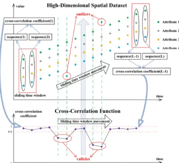
a one-dimensional correlation function by cross-correlation analysis, which also shows the idea of dimension reduction. Through selecting the values of each dimension at the same time we obtained a sequence, and two adjacent sequences are put into a sliding time window. A cross-correlation coefficient can be calculated for the two adjacent sequences in a sliding time window. With the shift of the sliding time window, we have a series of coefficients and obtain a cross-correlation function. As a result, the valley of the cross-correlation is the location of outliers.
Finally, for the outlier detection problem, it is difficult to determine the rank of the outlier and identify the rank thresh-olds. We investigate the multilevel Otsu’s method to provide a strategy for adaptive selection of the rank thresholds and hierarchical output of outliers based on the isolation degree of outliers. According to the cross-correlation function, each level of Otsu’s method can adaptively divide the data into two parts: normal points and outliers. Before executing the next level of the Otsu’s method, it will block the outliers which was found by the previous level, and continue to detect new outliers in the remaining normal points. Apparently, the ear-lier the outear-liers are detected, the higher the rank of them will be. Once the number of detected outliers reaches the outlier ratio threshold (the proportion of outliers to all data points in the dataset, which is preset by the user), the algorithm will stop the detection process. It is not necessary for users to set the rank thresholds of the cross-correlation function by using the multilevel Otsu’s method. In addition, it is very convenient to distinguish different outliers according to the isolation degree.
A set of experiments are performed to verify the valid-ity and reliabilvalid-ity of the proposed ODCA algorithm. Sev-eral typical high-dimensional real-world time series datasets containing both isolated and assembled outliers are used to test the proposed algorithm. Meanwhile, we also carry out some experiments to compare the effectiveness and time complexity of the ODCA algorithm with other five prevailing methods, and demonstrate the robustness of the proposed algorithm. Through the experimental results, it is shown that the ODCA algorithm can adaptively detect isolated and assembled outliers in high-dimensional time series datasets, and can output the detection results hierarchically with a shorter execution time and better detection effectiveness. In addition, it is very convenient for users because the outlier ratio threshold is only one parameter that should be preset.
The remainder of this paper is organized as follows. Section 2 gives a summary of recent researches for the outlier detection problem. The principle of the ODCA algorithm is presented in Section 3. The experiments and statistical results are presented and discussed in Section 4. Section 5 concludes the paper and points out further research directions.
II. RELATED WORK
There are a wide variety of strategies and algorithms for solving the outlier detection problem. We classify the outlier detection algorithms into ten types. They are respectively
based on statistics, regression, distance, density, clustering, filtering, wavelet transform, neural network, support vector machine and evolutionary algorithms.
Statistics-based methods were proposed by
Barnett and Lewis [20]. It determines outliers based on the inconsistency between the actual data and the ideal model. There are many algorithms based on different statistical
mod-els. For example, Brailovsky et al.[21] presented an
algo-rithm using a Bayes model. Gouriéroux [22] used an ARCH model to detect outliers in the field of finance. Monte-Carlo outlier detection was proposed by Zhanget al.[23] to estab-lish cross-prediction models for determining normal samples. Bouguessaet al.[24] investigated a principle approach based on the bivariate beta mixture model to identify outliers in mixed-attribute data. The statistics-based method has a high accuracy and a simple principle. However, it is necessary for users to know the distribution of datasets and the ideal model in advance, which is difficult in practical applications. It is the inherent weakness of the statistics-based method.
Regression-based methods are always suitable for detect-ing outliers in the time series dataset. Li and Li [25] applied a regression model to detect the outliers of energy consumption data of a real coke-oven plant to find an effective energy saving way for the plant. An improved outlier detection method using a regression model was presented in [26], and a synthesized signal using the measurements of different sensors was applied for estimating the model parameters. Kaneko [27] proposed a robust and automatic outlier sample detection method based on ensemble learning and regression analysis, and the outlier samples were detected by comprehensively considering multiple regression models.
Distance-based outlier detection techniques were proposed by Knorr and Ng [28]. The k-nearest-neighbor (KNN) clas-sification algorithm promoted the related researches [29]. The BIRCH algorithm proposed in [30] is aimed at finding k nearest neighbors. Kontakiet al.[31] introduced distance-based algorithms using sliding windows for continuous out-lier monitoring in data streams. Distance-based algorithms are very popular and fundamental in early studies, but they are very sensitive to parameter values. As a result, it is difficult to obtain the ideal detection result without prior knowledge of the data. In addition, it cannot distinguish the degree of isolation.
From a local point of view, density-based outlier detec-tion methods find outliers from datasets depending on the number of neighbors in a certain range and the degree of isolation within that range. Density-based outlier detection techniques were first proposed by Breuniget al.[32] using a local outlier factor (LOF) model. Therefore, the calculation of LOF became the core of the density-based outlier detec-tion technology. A LOF calculadetec-tion formula defined with probability density in the relevant subspace was presented
by Zhang et al. [33]. In order to increase the efficiency,
Bai et al. [34] split the dataset into several grids before calculating the LOF in parallel. In this way, users can find
global outliers and local outliers, but the time complexity is higher than other methods.
For detection algorithms based on clustering, the com-plement of the clustering result is the outlier set. In other words, abnormal samples are the by-products of clustering. The data points which are judged as outliers should satisfy one of the following two conditions: The point does not belong to any classes, or the size of the class is obviously smaller than the other classes. There are many achieve-ments in this area. An outlier detection method based on the
k-means algorithm was proposed by Lei et al. [35].
Jianget al.[36] introduced a strategy intended for the selec-tion of the initial cluster centers. Thah and Sitanggang [37] detected the outliers on hotspot data in Riau province using
k-means algorithm. Huanget al.[38], [39] added the
con-cept of natural neighbor to the cluster-based outlier detection algorithm so that the user would not need to decide the parameter value anymore. The outlier detection method based on clustering is an unsupervised learning method, but it is time-consuming and the detection efficiency is not high.
If we consider outliers as high frequency components in data sequences, the method based on filtering is the most direct way to solve the outlier detection problem. Using the dynamic filtering technology, the noise and outlier in the dataset can be weakened and replaced by normal val-ues so as to achieve the purpose of data preprocessing.
Chang et al. [40] used robust Kalman filtering to detect
outliers in time-series datasets dynamically. Moving-horizon estimation (MHE) was used to detect outliers for discrete-time linear systems by Alessandri and Awawdeh [41]. These methods are efficient and can deal with large amounts of data. However, the useful information hidden in the outliers will be filtered out automatically and the significance of outlier detection is lost.
The Lipschitz exponent in the wavelet transform theory can describe the singularity of function values. This kind of outlier detection method has been widely applied in many fields. For example, an outlier revision method of teleme-try data is proposed based on wavelet transformation by Ma and Liu [42]. Also, Wu and Li [43] proposed a method for satellite gravimetry data based on wavelet analysis. This method can identify a small number of assembled outliers, but cannot distinguish between noise and outliers.
As for using neural networks in outlier detection, it needs to be trained in advance. This method makes use of the learning ability of neural networks to realize the nonlinear mapping from input space to output space. Therefore, the problem of the uncertain relation among the attributes of data is solved. Neural networks can be used to solve classification and fitting problems. Both of them can be used in outlier detection. A Fuzzy min-max neural network, which is a hybridization of fuzzy and neural computing system, is used for outlier detection [44]. Barreto and Barros [45] introduced a simple and efficient extension to the extreme learning machine (ELM) network, which was very robust to label noise, a type of outlier occurring in classification tasks. The
FIGURE 1. Flowchart of the ODCA algorithm.
outstanding feature of ELM is that it is faster than the tra-ditional learning algorithm with similar learning accuracy, when compared with the traditional neural network.
Support vector machines (SVM) can be used in pattern recognition and classification, so they can also be applied for outlier detection. It uses the good classification perfor-mance of SVM to achieve outlier detection. The work in [46] presents a detailed analysis of various formulations of one-class SVM and uses them to separate the normal data from anomalous data in harsh environments. In consideration that the contribution yielded by the outlying instances and the nor-mal data is different, a robust one-class SVM which assigns an adapting weight for every object in the training dataset was proposed in [12]. These methods based on SVM also need further improvement because the detection results strongly depend on the choice of parameters and the origin of the coordinate.
In artificial intelligence, the evolutionary algorithm is a subset of evolutionary computation. In recent years, with the development of evolutionary algorithms, many people have applied them to outlier detection. For example, a genetic algo-rithm to detect multiple additive outliers in multivariate time series was proposed in [47]. In [48], an outlier was considered as a deviation which indicates the existence of cancerous cells in the breast, and the authors proposed a new approach to out-lier detection based on the multi-objective genetic algorithm. Not only genetic algorithms, particle swarm optimization can also be used for outlier detection. Ye and Chen [49] pre-sented an algorithm for outlier detection in high-dimensional spaces based on constrained particle swarm optimization techniques.
In general, there are many sophisticated methods for out-lier detection. These complementary methods perform well in outlier detection for specific problems. However, there are several problems that need to be addressed. First, low
efficiency with high time complexity is the most primary problem. Second, some algorithms are sensitive to the thresh-old of corresponding parameters which are set by users. Third, the degree of abnormality cannot be distinguished. Fourth, the detection results are not satisfactory when dealing with high-dimensional datasets. Finally, the assembled out-liers cannot be detected by existing methods.
These problems limited our ability to apply outlier detec-tion methods to high-dimensional time series datasets that contain both isolated and assembled outliers. Inspired by the existing methods, we propose a new outlier detection method named ODCA to address these limitations.
III. THE ODCA ALGORITHM
In this paper, we propose an outlier detection algorithm framework based on cross-correlation analysis. Several steps are designed to detect outliers for time series datasets. First, linear interpolation is used to scatter the assembled outliers in the dataset and preprocess the data. Second, in the process of analyzing outliers, the cross-correlation function of adja-cent sequences is obtained when the sliding time window is moving. Third, the thresholds of cross-correlation function are adaptively selected using the multilevel Otsu’s method, the process of which is called outlier rank. Finally, when the number of detected outliers reaches the preset proportion, the algorithm stops and outputs the detection results hier-archically. The detailed process of the algorithm is shown in Fig.1.
A. DATA PREPROCESSING
1) ISOLATED OUTLIERS AND ASSEMBLED OUTLIERS
The outliers for the real world problems can be divided into two categories according to their distribution range. They are the isolated outliers and the assembled outliers.
FIGURE 2. The definition and comparison of the isolated outliers and the assembled outliers.
The isolated outliers refer to the outliers that appear indi-vidually, which means any two isolated outliers are located far apart from each other in time. In other words, the data points in the neighborhood of isolated outliers are all normal data values.
However, the assembled outliers refer to a small number of outliers that flock together. It means that the data points in a tiny time window are all outliers. Usually, since outliers are only a small part of the dataset, the length of this tiny time window will be much smaller than the length of the dataset. In this algorithm, we take the length of the time window as 1/1000 of the length of the dataset. The definition and comparison of the isolated outliers and the assembled outliers are shown in Fig.2.
For isolated outliers, they can be detected directly by cross-correlation analysis, which will be explained in Section 3.2. For assembled outliers, they themselves may follow some unique distributions, such as the random distribution or the same tendency with normal data points but a large differ-ence in mean value. Eventually, they will affect the envelope shape of the cross-correlation function, which may lead to the inaccurate location of the outliers. For example, as shown in Fig.3, two isolated outliers which are close to each other and randomly distributed assembled outliers will correspond to a similar cross-correlation function. Therefore, we use the linear interpolation method in data preprocessing to con-vert assembled outliers to isolated outliers, which can be detected using the cross-correlation analysis more easily and unambiguously. The reason for using linear interpolation in data preprocessing to convert assembled outliers to isolated outliers is shown in Fig.3.
2) LINEAR INTERPOLATION
Linear interpolation is the process of determining or predict-ing the unknown points by uspredict-ing a line connectpredict-ing two known points [50]. Assuming that the coordinates of two known points are (x0,y0) and (x1,y1), we need to obtain theyvalue
of any point in the interval [x0,x1]. The principle of linear
interpolation is shown in Fig.4.
Here, we define the interpolation coefficient β, which
refers to the number of inserted points in (1).
β = y−y0
y1−y
= x−x0
x1−x
(1)
FIGURE 3.The reason for using linear interpolation in data preprocessing.
FIGURE 4. The principle of linear interpolation.
It denotes the ratio between the distance fromx0toxand
the distance fromxtox1. For example, if we need to insert
two data samples evenly between two known points, the
inter-polation coefficient should beβ =2. Fig.5 shows the effect
of linear interpolation when the interpolation coefficientβis equal to 2. In Fig.5, the data points with the black circle marks are the interpolation points.
3) DATA PREPROCESSING ALGORITHM
The data preprocessing can be divided into the following steps. First, the pruning strategy is used to determine the normal points which must not be outliers in the dataset. Then, these normal points are used to interpolate the data linearly so that the normal points are inserted between the assembled outliers. Finally, the problem is transformed into a case of isolated outliers. The pseudo code of data preprocessing is shown as follows.
The design of the pruning strategy mainly considers two characteristics of normal data points. First, the cross-correlation coefficient of normal points should be relatively high. However, the assembled outliers which follow the same
FIGURE 5. The effect of linear interpolation.
Algorithm 1Data Preprocessing (Linear Interpolation)
Require: Dis the time series dataset, size:L∗N
Ensure: D0is the interpolated time series dataset, size: (3∗
L−1)∗N
STEP 1: Pruning Strategy
Determining the normal points which must not be outliers
STEP 2: Linear Interpolation
Inserting the normal points between the assembled outliers
tendency and distribution with normal data points may also satisfy this feature. Therefore, we also need to examine the cross-correlation coefficient of the neighborhood of the specific data object. In summary, the feature of the data points which must not be outliers should be that the cross-correlation coefficients of all data points in the neighborhood are relatively high. Here, the size of the neighborhood should be larger than the length of the time window which was mentioned when defining the assembled outliers, so that the assembled outliers will not be regarded as normal values. In this algorithm, we take the size of the neighborhood as 1/100 of the length of the dataset.
In order to turn the assembled outliers into isolated out-liers which can be detected, the setting of the appropriate interpolation coefficient is a crucial problem worth consid-ering. Detailed illustrations about the resolution interval are shown in Fig.6. It is worth noting that an isolated outlier in the dataset will map to two valley values in the cross-correlation function. Therefore, when the cross-cross-correlation function has four adjacent valley values, just as the condition shown in Fig.6, the algorithm cannot judge whether there are two isolated outliers or there are three assembled outliers. When interpolation is not performed or the interpolation coefficientβ is 1, the situation of isolated points is ambigu-ous. However, if we insert two normal points, the assembled outliers can be completely separated. It means that as long as there are two normal data points between two adjacent
FIGURE 6. The selection of the linear interpolation coefficient.
isolated outliers, the algorithm is able to detect them. There-fore, the proper value of the linear interpolation coefficientβ is 2.
B. OUTLIER ANALYSIS
1) PEARSON PRODUCT-MOMENT CORRELATION COEFFICIENT
The cross-correlation coefficient rxy is a parameter that
describes the similarity between two random variables, X and Y. Both X and Y are N dimensional vectors here. That is,X = (x1,x2,x3, ...,xN) andY = (y1,y2,y3, ...yN). The
correlation coefficient, proposed by British scientist Pear-son [51] in 1880, is widely used in various fields. In this paper, Pearson product-moment correlation coefficient (PPCC) is applied. The calculation formula of PPCC is as follows.
rxy= PN i=1(xi−X)(yi−Y) q PN i=1(xi−X)2 q PN i=1(yi−Y)2 (2)
According to the theory of cross-correlation analysis, the closer the values of two discrete sequences are, the higher the correlation coefficient is. Once the values of the two sequences vary greatly at a certain time, the value of the cross-correlation coefficient will significantly reduce. For example, the first sequence is {1,2,3,4,5} and the second sequence is {1.1,2.1,3.1,4.1,5.1}, which is extremely famil-iar with the first one. In this case, the cross-correlation coefficient is 0.9999. But if the second sequence becomes {1.1,2.1,10,4.1,5.1}, in other words, the third element in this sequence is an outlier, the correlation coefficient will apparently decrease to 0.8544.
FIGURE 7. The process of cross-correlation analysis.
2) OUTLIER ANALYSIS ALGORITHM
For the high-dimensional time series dataset, there is no obvious correlation among the data of different attributes, but there should be a certain continuity between the data at adjacent times. Considering the continuity and correlation of data at adjacent times, cross-correlation analysis can be applied to detect outliers.
The values of each dimension at the same time can form a sequence. The adjacent two sequences are selected as a sliding time window. The cross-correlation coefficient of the two adjacent sequences in one sliding time window can be calculated as one point of the cross-correlation function. Assuming that the length of the high-dimensional time series dataset is L, as the sliding time window moves at interval of one step, a cross-correlation function with L-1 points can be obtained.
Actually, it is one kind of dimension-reduction process, which maps the outliers in the high-dimensional dataset to the one-dimensional cross-correlation function. There may be outliers at the valley of the cross-correlation function because the cross-correlation coefficient reflects the simi-larity of the adjacent sequences. The outliers differ greatly from the normal data values both on the left and right sides, so an outlier will correspond to the two valley values of the cross-correlation function, which requires further comparison of the data values in the neighborhood to lock the location of the outliers. The whole analysis process using the cross-correlation function is shown in Fig.7.
The pseudo code of cross-correlation analysis is shown as follows.
C. OUTLIER RANK
Actually, there is usually continuity between the normal points and the outliers. It is not reasonable to directly define
Algorithm 2Outlier Analysis (Cross-Correlation Analysis)
Require: D0is the interpolated time series dataset, size: (3∗
L−1)∗N
Ensure: CF0 is the cross-correlation function of the interpo-lated dataset, size: (3∗L−1)∗1
STEP 1: Controlling Range
Limiting the data values between 0 and 10
STEP 2: Forming Sequence
Refering to the data of each dimension at the same time
STEP 3: Calculating Correlation Coefficient
Calculating the correlation coefficient of two adjacent sequences in one time window
STEP 4: Sliding Time Window
Moving the time window at interval of 1 step
STEP 5: Forming Correlation Function
Generating a cross-correlation function with L-1 points
a data point as an outlier or a normal point. Therefore, it is better to mark or rank the detected outliers according to the isolation degree. In fact, the outlier detection algorithm needs the ability to select the rank thresholds adaptively. It means that the adaptive selection of thresholds and the hierarchical output of outliers are two problems that must be solved.
1) Otsu’s METHOD
Otsu’s method was firstly proposed by Japanese scholar Otsu [52] in 1979 and was widely used in the field of digital image processing to distinguish foreground and background [53]. It divides the sample points into two cat-egories by the principle of the maximum variance between classes and the minimum variance within classes, and gives the threshold of classification adaptively.
Specifically, if the ratio of the foreground points and the background points to the whole image are respectively
expressed as w0 and w1, and the mean gray value of the
foreground points and the background points are respectively expressed asu0 and u1, then the average gray level of the
whole imageuand the inter-class variance of the foreground
and background points σ can be respectively calculated
as (3) and (4). In Otsu’s method, we exhaustively search for the classification threshold that minimizes the inter-class varianceσ by traversing the classification threshold from the minimum gray value to the maximum gray value.
u =w0∗u0+w1∗u1 (3) σ =w0∗(u0−u)2+w1∗(u1−u)2 (4) 2) OUTLIER RANK ALGORITHM
In this paper, we investigate the Otsu’s method in the adaptive threshold selection, and design a multilevel Otsu’s method to classify the amplitude of cross-correlation function and output the detection results hierarchically. It should be noted that the classification object of the multilevel Otsu’s method
FIGURE 8. The process of the multilevel Otsu’s method.
is the set of cross-correlation coefficients, rather than the dataset. The principle and procedures of the multilevel Otsu’s method are introduced below.
To begin with, the outliers generated by the first classifica-tion are called level-one outliers, and the remaining normal data will be classified again. Then, we repeat the above steps and gradually screen out outliers at different levels, until the number of outliers reached the predetermined proportion. Finally, the threshold of the last Otsu’s method is taken as the final classification threshold. The implementation steps of the first two stages of the Otsu’s method are shown in Fig.8.
The pseudo code of the multilevel Otsu’s method is shown as follows.
Algorithm 3Outlier Rank (Multiple Otsu’s Method)
Require: CF0 is the cross-correlation function of the interpo-lated time series dataset, size: (3∗L−1)∗1;
ONT is the outlier number threshold entered by the
user
Ensure: CCT is a set of the cross-correlation thresholds of each level;
ODRis a set of the detected outliers classified by level
STEP 1: Otsu’s method
Classifing the amplitude of cross-correlation function and outputting outliers of the current level
STEP 2: Decision Criterion
Going back to step 1 if the number of outliers doesn’t reach the preset value
It should be noted that the outlier threshold, which refers to the proportion of the outliers in the dataset, is the only param-eter needs to be preset by the user in our algorithm. All of the thresholds in the process of outlier rank can be selected by the multilevel Otsu’s method adaptively. Sensitivity analysis of the outlier threshold is presented in Section 4.5.
D. EVALUATION MODEL
We use three kinds of models to evaluate the ODCA algorithm in different aspects. First, confusion matrix can compare the predicted results with the actual results of the outlier detec-tion. Second, the coefficientJ can be calculated by the four elements of the confusion matrix, which will be more suitable for the outlier detection problem. Third, receiver operating
TABLE 1.The construction of the confusion matrix.
characteristic (ROC) curve can describe the classifier effec-tiveness more intuitively in a two-dimensional plane.
1) CONFUSION MATRIX
The construction of the confusion matrix is shown in Table 1 [54].
Class TP is the most common set of the normal data points and has little impact on the detection algorithm. Class FN contains data points which are not outliers, but are detected as outliers. It exists because the threshold proportion of the outliers in the algorithm is so large that some normal points are considered as outliers. Class FP refers to the data which was originally abnormal but has not been detected. On the contrary, it exists because the threshold proportion is too small which leads to the missing outliers. Class TN refers to the data which was originally abnormal and detected at the same time.
2) THE COEFFICIENTJ
The calculation process of the coefficientJ is based on the
confusion matrix. Class FN and Class FP affect the effec-tiveness of the whole algorithm. The fewer the data points in FN and FP classes, the better the algorithm is. The optimal result is that class FN and class FP is minimized, and the class TN is maximized close to the total number of outliers.
We define the coefficientJ as the outlier detection eval-uation factor, which is the ratio of the number of detected outliers to the size of the dataset. Class TP is the normal data which accounts for most of the dataset. The larger the size of class TP, the smaller the influence on the evaluation coefficient. If theJis too small, the evaluation coefficient will be clustered around 0, which cannot reflect the difference of detection results. Therefore, it is not necessary to consider the influence of the normal dataset on the evaluation coefficient. Therefore, the calculation of the evaluation coefficient can be simplified in (5). J = TN TP+FN+FP+TN ⇒ TN FN+FP+TN = 1 1+FN+FP TN (5)
FIGURE 9. The formation of the ROC curve.
We can find that the evaluation coefficientJ is inversely proportional to the data amount of FN and FP classes, and is proportional to the data amount of TN class. The larger the evaluation coefficient J, the higher the effectiveness of the
algorithm. WhenJ= 1, both FN and FP are equal to 0, which
shows that the outlier detection results are optimal.
3) ROC CURVE
In statistics, ROC curve is a graphical plot that illustrates the diagnostic ability of a binary classifier system as its discrimination threshold is varied [55]. The ROC curve is created by plotting the true positive rate (TPR) against the false positive rate (FPR) at various thresholds. The formation of the ROC curve is shown in Fig.9.
The TPR is also known as sensitivity, recall or probability of detection, and the FPR is also known as the fall-out or prob-ability of false alarm. TPR and FPR can be calculated by (6) and (7).
TPR= TP
TP+FN (6)
FPR= = FP
FP+TN (7)
IV. EXPERIMENT AND ANALYSIS
We select two small-scale modeling time series datasets and two large-scale representative real-world time series datasets to evaluate the feasibility of the proposed ODCA algorithm. The two small-scale datasets are the population dataset and the receiver dataset. The population dataset is about the pop-ulation of ten countries from 1953 to 2008. The receiver dataset is the position and velocity information decoded by the satellite navigation receiver. The two large-scale datasets are the climate dataset and the house condition dataset. The climate dataset is the hourly climate data recorded from January 1st, 2010 to December 30th, 2015 in Beijing. The house condition dataset is the house temperature and humid-ity conditions monitored by a ZigBee wireless sensor net-work. For the convenience of the experiments, we artificially
FIGURE 10. The original data distribution in Experiment 1.
inserted several outliers, whose positions and values are cho-sen arbitrarily to illustrate the performance of different outlier detection algorithms.
In addition, we investigate two kind of further experiments based on the house condition dataset, which is more represen-tative among these four datasets. On one hand, we compare our algorithm with some prevailing algorithms in terms of detection effectiveness and execution time. These algorithms are the methods based on wavelet analysis, bilateral filtering, particle swarm optimization, auto-regression and extreme learning machine. On the other hand, we discuss the influence of the noise in the dataset on the performance of our proposed algorithm.
All of the following experiments are performed under the MATLAB simulation environment.
A. EXPERIMENT 1: THE POPULATION DATASET
The population dataset includes the population of ten countries from 1953 to 2008, namely, Australia, Brazil, Canada, China, Egypt, France, Germany, Japan, the United Kingdom and the United States [56]. The dataset con-sists of 10 attributes and 56 objects. With the year as the horizontal axis and the population of each country as the vertical axis, the original data distribution is shown in Fig.10.
Here, we directly insert 3 isolated outliers and 3 assembled outliers into the dataset. They are located in the 9th object of the 4th attribute, the 19th object of the 7th attribute, the 37th object of the 9th attribute and the 46th to the 48th objects of the 10th attribute. The outlier detection result and the cross-correlation function are shown in Fig.11 and Fig.12, respectively.
After the linear interpolation process, the assembled out-liers are separated by normal points so that they can be transformed into isolated outliers. It is not difficult to find from Fig.12 that the 6 outliers correspond to the 6 obvious valley values of the cross-correlation function. The result of the hierarchical output are shown in Table 2.
It can be seen from Table 2 that, before the number of detected outliers reaches the preset value, the multilevel
FIGURE 11. The outlier detection result in Experiment 1.
FIGURE 12. The cross-correlation function in Experiment 1.
TABLE 2. The result of the hierarchical output in Experiment 1.
Otsu’s method has executed 3 times. The Otsu’s method at each level can adaptively determine the classification threshold according to the current cross-correlation coeffi-cients distribution, and output the outliers of each level. It is apparent that the detection result is reasonable by means of comparing Fig.11 and Table 2. The higher the outlier level is, the greater the outlier deviates from the normal value. Since all the outliers have been detected, the evaluation coefficient
Jis equal to 1. The detection result shows that the algorithm can detect all the isolated outliers and the assembled outliers in the high-dimensional time series dataset, output them hier-archically, locate them in the dataset, and mark them on the data image.
FIGURE 13. The original data distribution in Experiment 2.
FIGURE 14. The outlier detection result in Experiment 2.
B. EXPERIMENT 2: THE RECEIVER DATASET
The dataset recorded by a satellite navigation receiver in our laboratory consists of 1000 objects and 5 attributes, namely, week, longitude, latitude, height and speed. With the time as the horizontal axis and the value of each attribute as the vertical axis, the original data distribution is shown in Fig.13.
Here, we directly insert 4 isolated outliers and 4 assembled outliers into the dataset. They are located in the 933rd object of the 1st attribute, the 282th object of the 2nd attribute, the 463rd to 466th objects of the 3st attribute, the 122nd object of the 4th attribute and the 795th object of the 5th attribute. The outlier detection result and the cross-correlation function are shown in Fig.14 and Fig.15, respectively.
The result of the hierarchical output are shown in Table 3. From Fig.13, we can see that the continuity of the receiver dataset is not as good as the population dataset. However, the valley value of the cross-correlation function is still very evident. Since all the outliers have been detected, the evalua-tion coefficientJis equal to 1. In the result, cross-correlation analysis and the linear interpolation algorithm can still detect all of the isolated and assembled outliers, and the multilevel Otsu’s method output them hierarchically.
C. EXPERIMENT 3: THE CLIMATE DATASET
The hourly climate dataset consists of 50048 objects
and 3 attributes, namely, dew point, pressure and
FIGURE 15. The cross-correlation function in Experiment 2.
TABLE 3. The result of the hierarchical output in Experiment 2.
FIGURE 16. The original data distribution in Experiment 3.
the value of each attribute as the vertical axis, the original data distribution is shown in Fig.16.
Here, we directly insert 3 isolated outliers and 3 assembled outliers into the dataset. They are located in the 13300th and the 25000th object of the 1st attribute, the 45000th object of the 2nd attribute and the 27000th to the 27002nd objects of the 3rd attribute. The outlier detection result and the cross-correlation function are shown in Fig.17 and Fig.18, respectively.
The result of the hierarchical output are shown in Table 4. Compared with the small-scale datasets in the above two experiments, the climate dataset is closer to the actual
FIGURE 17. The outlier detection result in Experiment 3.
FIGURE 18. The cross-correlation function in Experiment 3.
TABLE 4.The result of the hierarchical output in Experiment 3.
situation in data capacity. Even so, the ODCA algorithm can still detect several abnormal samples according to the outlier ratio threshold set by the user. Since all the outliers have been detected, the evaluation coefficientJis equal to 1. Thus, the algorithm has good robustness properties and detection performance for large scale datasets.
D. EXPERIMENT 4: THE HOUSE CONDITION DATASET
The house conditions dataset consists of 19735 objects and 12 attributes, namely, the temperature and humidity of the kitchen, living room, laundry room, office room, bathroom and outside of the building [60]. With the time as the hori-zontal axis and the value of each attribute as the vertical axis, the original data distribution is shown in Fig.19.
Here, we directly insert 11 isolated outliers and 3 assem-bled outliers into the dataset. They are located in the 17500th object of the 1st attribute, the 5500th and the 14404th objects
FIGURE 19. The original data distribution in Experiment 4.
FIGURE 20. The outlier detection result in Experiment 4.
FIGURE 21. The cross-correlation function in Experiment 4.
of the 2nd attribute, the 5000th object of the 3rd attribute, the 13825th object of the 4th attribute, the 10000th to the 10002nd objects of the 5th attribute, the 12000th object of the 6th attribute, the 7500th object of the 7th attribute, the 2600th object of the 8th attribute, the 2500th object of the 10th attribute, the 12912th object of the 11th attribute and the 19000th object of the 12th attribute. The outlier detection result and the cross-correlation function are shown in Fig.20 and Fig.21, respectively.
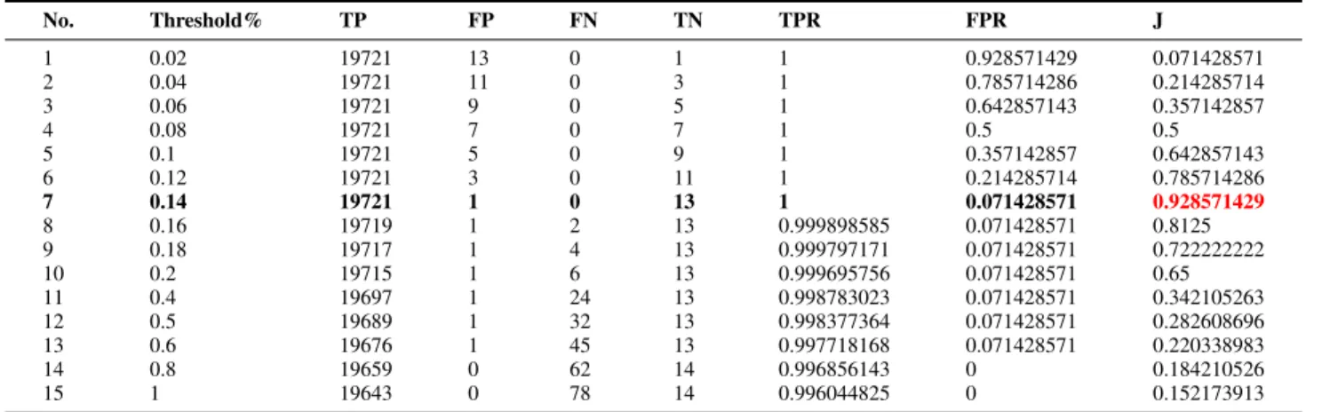
The result of the hierarchical output are shown in Table 5. The dataset in this experiment is more complex in dimen-sion, and it is the most challenging problem in the four experiments. As for the 14 outliers inserted artificially, the
TABLE 5.The result of the hierarchical output in Experiment 4.
proposed outlier detection algorithm can still detect 13 out-liers, and only 1 of them is missing. The evaluation
coeffi-cientJ is equal to 0.9286. Because the isolated degrees of
these detected outliers are similar, in other words, the correla-tion coefficients of them are close to each other, the algorithm does not classify them further in different ranks.
E. PERFORMANCE COMPARISON
For further evaluating the performance of the proposed ODCA algorithm, we compare the algorithm with other methods for time series, namely, the methods based on the Wavelet Analysis (WA), Bilateral Filtering (BF), Parti-cle Swarm Optimization (PSO), Auto-Regression (AR) and Extreme Learning Machine (ELM). The evaluation pro-cess consists of two aspects, the effectiveness and the time complexity.
1) EFFECTIVENESS
We test the effectiveness of the ODCA algorithm and other methods based on WA, BF, PSO, AR and ELM in the case of different outlier thresholds (different populations in PSO-based method) using the house condition dataset, which is the most challenging one among four datasets. The statis-tical results are shown in Table 6, Table 7, Table 8, Table 9, Table 10 and Table 11, respectively.
The bold row in these six tables represents the situa-tion when the six outlier detecsitua-tion algorithms are optimal. By comparing the optimal condition of the six algorithms, we can find in Fig.22 that the ODCA algorithm has the best performance among them.
For a more intuitional comparison, the effectiveness for different algorithms is presented in the form of J curve and ROC curve in Fig.23 and Fig.24.
In fact, the closer to 1 the value of the coefficient J is, the better the effectiveness of the algorithm is. As for the ROC curve, the closer to the upper-left border of the ROC space the ROC curve is, the more accurate the detection result is. In addition, the area under the curve is a measure of classifi-cation accuracy. It should be pointed out that, in Fig.23, when the size of the population in the algorithm based on PSO is
TABLE 6. The effectiveness of the ODCA algorithm in the case of different outlier thresholds.
TABLE 7. The effectiveness of the algorithm based on WA in the case of different outlier thresholds.
TABLE 8. The effectiveness of the algorithm based on BF in the case of different outlier thresholds.
getting larger, the effectiveness of this method will be better. However, the executing time is also becoming longer, which will be illustrated in detail in Section 4.5.2. Therefore, com-pared with other methods, the ODCA algorithm has better detection effectiveness.
2) TIME COMPLEXITY
In addition, we compare the running time of the above-mentioned methods with that of the ODCA algorithm when the length (L) and dimension (N) of test datasets changed, which is presented in Fig.25.
TABLE 9. The effectiveness of the algorithm based on PSO in the case of different populations.
TABLE 10. The effectiveness of the algorithm based on AR in the case of different outlier thresholds.
TABLE 11. The effectiveness of the algorithm based on ELM in the case of different outlier thresholds.
We can find that the execution time of our algorithm is shorter than the methods based on BF, PSO, AR and ELM, and is a little bit longer than the method based on WA. The method based on wavelet transform analyzes the approxi-mation degree of the signal and the wavelet function using the inner product, whereas the ODCA algorithm uses the cross-correlation coefficient to represent the similarity of the adjacent sequences. The inner product operation only con-tains multiplication and addition. The calculation of cross-correlation coefficient includes not only multiplication and addition, but also some complex operations such as division and square root. As a result, the execution time of cross-correlation analysis is a little longer than that of wavelet analysis.
It is worth noting that the execution time of the ODCA algorithm does not grow with the increase of the dimension
of the dataset, which is a significant advantage that other algorithms do not have.
In fact, the time complexities of cross-correlation anal-ysis, linear interpolation and the multilevel Otsu’s method are all O(l). Therefore, the time complexity of the whole outlier detection algorithm is alsoO(l), which is much smaller than that of other outlier detection algorithms. The time complexity of statistic-based method [20], distance-based method [28], [31], clustering-based method [30], [35], [36], density-based method [32], [34], SVM-based method [44], [45] and other algorithms used to detect outliers in the time series dataset [12], [17]–[19], [21], [25]–[27], [40]–[42], [46], [47] are compared in Table 12.
In Table 12, n represents the data dimension, l
rep-resents the data length, and c represents the number of
FIGURE 22. Comparison of the optimal effectiveness.
TABLE 12. The time complexity of various outlier detection algorithms.
F. ROBUSTNESS ANALYSIS
In order to analyze the robustness of the proposed algorithm, we carried out an experiment about the influence of noise on detection results for the housing condition dataset. We added white Gaussian noise (WGN) of different power to the hous-ing condition dataset, and record the J coefficients of the detection algorithm. The result of the experiment is shown in Table 13 and Figure 26.
After analyzing the experiment result and fitting the data, we can conclude that as the noise of the dataset increases, the detection performance of the algorithm will decrease in the form of three-order polynomials approximately. When the
FIGURE 23. TheJcurve.
FIGURE 24. The ROC curve.
dataset contains low power noise (less than 26 dBm), the coef-ficient J decreases at a slow rate and the performance of our algorithm will not be greatly affected, which indicates that the ODCA algorithm has good robustness. However, if the power of the noise is too large (more than 30 dBm), the data will be submerged in heavy noise and the continuity of time series datasets will be destroyed, which is the base of our ODCA method. As a result, the performance of the outlier detection may not be satisfactory. Nevertheless, considering the impact of noise on detection results is a common issue for all outlier detection algorithms, our algorithm will still perform better compared with other methods under the same noisy condition.
G. SUMMARY
Based on the experimental results and the comparison with other algorithms, we can find that the ODCA algorithm demonstrates good applicability for both small-scale datasets and large-scale datasets. Also, ODCA is a one-parameter algorithm because the outlier ratio threshold is the only parameter that needs to be chosen by the user, and the outlier rank thresholds are all selected automatically using the multilevel Otsu’s method. Besides, from the ROC curve and the J curve, the ODCA algorithm performs better than other methods for the same dataset. Furthermore, the exe-cution time of the ODCA algorithm does not increase with
FIGURE 25. The time curve.
TABLE 13. The influence of noise on detection result.
FIGURE 26. The influence of noise on detection result.
the dimension of the dataset, which determines that the proposed algorithm will be more suitable for dealing with high-dimensional datasets than other methods. In addition, the proposed method has good robustness when the dataset contains noise. Overall, the ODCA algorithm is better than other outlier detection algorithms in terms of applicability, effectiveness, time complexity and robustness.
V. CONCLUSION
The outlier detection in time series datasets is a very important problem in practical applications. We propose a new algorithm named ODCA to detect outliers in high-dimensional time series datasets. The method contains three parts. First, data preprocessing based on linear interpola-tion can transform assembled outliers into isolated outliers. Second, outlier analysis based on cross-correlation analysis can map the outliers of the high-dimensional dataset to one-dimensional cross-correlation function, the valley of which corresponds with the location of outliers. Third, outlier rank based on the multilevel Otsu’s method can adaptively deter-mine the rank thresholds and realize the hierarchical output according to the isolation degree of the outliers. The sta-tistical results of different experiments illustrate the strong detection capability for high-dimensional time series datasets containing both isolated and assembled outliers by using the proposed ODCA algorithm.
Our future work will focus on a parameter-less outlier detection algorithm. Currently the user still needs to set the outlier ratio threshold, which requires a prior knowledge of the dataset. We will develop domain-specific algorithms to fully achieve the adaptive selection of thresholds. Also, we find that the process of constructing the cross-correlation
function by calculating the cross-correlation coefficients can be handled in parallel. Therefore, we can use parallel process-ing platforms, such as GPU, to further reduce the program execution time.
REFERENCES
[1] M. Hauskrecht, I. Batal, M. Valko, S. Visweswaran, G. F. Cooper, and G. Clermont, ‘‘Outlier detection for patient monitoring and alerting,’’ J. Biomed. Inform., vol. 46, pp. 47–55, Feb. 2013.
[2] A. Christy, G. M. Gandhi, and S. Vaithyasubramanian, ‘‘Cluster based outlier detection algorithm for healthcare data,’’Procedia Comput. Sci., vol. 50, pp. 209–215, Jan. 2015.
[3] Z. Xie, X. Li, W. Wu, and X. Zhang, ‘‘An improved outlier detection algorithm to medical insurance,’’ inIntelligent Data Engineering and Automated Learning, H. Yin, Y. Gao, B. Li, D. Zhang, M. Yang, and Y. Li, Eds. Cham, Switzerland: Springer, 2016, pp. 436–445.
[4] N. Carneiro, G. Figueira, and M. Costa, ‘‘A data mining based system for credit-card fraud detection in e-tail,’’Decis. Support Syst., vol. 95, pp. 91–101, Mar. 2017.
[5] S. Subudhi and S. Panigrahi, ‘‘Use of optimized fuzzy C-means clus-tering and supervised classifiers for automobile insurance fraud detec-tion,’’ J. King Saud Univ.—Comput. Inf. Sci., to be published, doi:
10.1016/j.jksuci.2017.09.010.
[6] W. Da and H. S. Ting, ‘‘Distributed intrusion detection based on out-lier mining,’’ inProc. Int. Conf. Commun., Electron. Automat. Eng., G. Yang, Ed. Berlin, Germany: Springer, 2013, pp. 343–348.
[7] T. Li and N.-F. Xiao, ‘‘Novel heuristic dual-ant clustering algorithm for network intrusion outliers detection,’’Optik—Int. J. Light Electron Opt., vol. 126, pp. 494–497, Feb. 2015.
[8] H. Zhao, B. Jiang, J. Tang, and B. Luo, ‘‘Image matching using a local distribution based outlier detection technique,’’Neurocomputing, vol. 148, pp. 611–618, Jan. 2015.
[9] I. H. Lee and M. T. Mahmood, ‘‘Adaptive outlier elimination in image registration using genetic programming,’’Inf. Sci., vol. 421, pp. 204–217, Dec. 2017.
[10] H. Palus and M. Frackiewicz, ‘‘Colour image quantisation using KM and KHM clustering techniques with outlier-based initialisation,’’ in Developments in Medical Image Processing and Computational Vision, J. M. R. S. Tavares and R. N. Jorge, Eds. Cham, Switzerland: Springer, 2015, pp. 261–278.
[11] A. Abid, A. Masmoudi, A. Kachouri, and A. Mahfoudhi, ‘‘Outlier detec-tion in wireless sensor networks based on OPTICS method for events and errors identification,’’Wireless Pers. Commun., vol. 97, pp. 1503–1515, Nov. 2017.
[12] N. Shahid, I. H. Naqvi, and S. B. Qaisar, ‘‘One-class support vec-tor machines: Analysis of outlier detection for wireless sensor net-works in harsh environments,’’Artif. Intell. Rev., vol. 43, pp. 515–563, Apr. 2015.
[13] P. Gil, H. Martins, and F. Januário, ‘‘Outliers detection methods in wireless sensor networks,’’Artif. Intell. Rev., vol. 49, p. 126, Feb. 2018. [14] M. Cejnek and I. Bukovsky, ‘‘Concept drift robust adaptive novelty
detection for data streams,’’ Neurocomputing, vol. 309, pp. 46–53, Oct. 2018.
[15] F. Battaglia, ‘‘Outliers in functional autoregressive time series,’’Statist. Probab. Lett., vol. 72, pp. 323–332, May 2005.
[16] M. E. Silva and I. Pereira, ‘‘Detection of additive outliers in Poisson integer-valued autoregressive time series,’’Statistics, Apr. 2012. [Online]. Available: http://arxiv.org/pdf/1204.6516.pdf
[17] T. Bellini, ‘‘The forward search interactive outlier detection in cointegrated VAR analysis,’’Adv. Data Anal. Classification, vol. 10, pp. 351–373, Sep. 2016.
[18] R. Baragona, F. Battaglia, and D. Cucina, ‘‘Empirical likelihood for outlier detection and estimation in autoregressive time series,’’J. Time Ser. Anal., vol. 37, no. 3, pp. 315–336, 2016.
[19] L. Bardwell and P. Fearnhead, ‘‘Bayesian detection of abnormal segments in multiple time series,’’Bayesian Anal., vol. 12, no. 1, pp. 193–218, 2015. [20] V. Barnett and T. Lewis,Outliers in Statistical Data, 3rd ed. New York,
NY, USA: Wiley, 1994.
[21] V. L. Brailovsky, ‘‘An approach to outlier detection based on Bayesian probabilistic model,’’ inProc. Int. Conf. Pattern Recognit., Aug. 1996, pp. 70–74.
[22] C. Gouriéroux,ARCH Models and Financial Applications. New York, NY, USA: Springer, 1997.
[23] L. Zhanget al., ‘‘Improvement on enhanced Monte–Carlo outlier detection method,’’Chemometrics Intell. Lab. Syst., vol. 151, pp. 89–94, Feb. 2016. [24] M. Bouguessa, ‘‘A practical outlier detection approach for mixed-attribute
data,’’Expert Syst. Appl., vol. 42, no. 22, pp. 8637–8649, 2015. [25] L. Li and T. Li, ‘‘A case study on regression model based outlier detection,’’
inAdvances in Information Technology and Industry Applications. Berlin, Germany: Springer, 2012, pp. 661–669.
[26] C. M. Park and J. Jeon, ‘‘Regression-based outlier detection of sensor measurements using independent variable synthesis,’’ inData Science. Cham, Switzerland: Springer, 2015, pp. 78–86.
[27] H. Kaneko, ‘‘Automatic outlier sample detection based on regression analysis and repeated ensemble learning,’’Chemometrics Intell. Lab. Syst., vol. 177, pp. 74–82, Jun. 2018.
[28] E. M. Knorr and R. T. Ng, ‘‘Algorithms for mining distance-based outliers in large datasets,’’ inProc. Int. Conf. Very Large Data Bases, 1998, pp. 392–403.
[29] R. F. Sproull, ‘‘Refinements to nearest-neighbor searching in k-dimensional trees,’’Algorithmica, vol. 6, pp. 579–589, Jun. 1991. [30] T. Zhang, R. Ramakrishnan, and M. Livny, ‘‘BIRCH: An efficient data
clustering method for very large databases,’’ inProc. ACM SIGMOD Int. Conf. Manage. Data, 1996, pp. 103–114.
[31] M. Kontaki, A. Gounaris, A. N. Papadopoulos, K. Tsichlas, and Y. Manolopoulos, ‘‘Efficient and flexible algorithms for monitoring distance-based outliers over data streams,’’Inf. Syst., vol. 55, pp. 37–53, Jan. 2016.
[32] M. M. Breunig, H.-P. Kriegel, and R. T. Ng, ‘‘LOF: Identifying density-based local outliers,’’ inProc. ACM SIGMOD Int. Conf. Manage. Data, 2000, pp. 93–104.
[33] J. Zhang, X. Yu, Y. Li, S. Zhang, Y. Xun, and X. Qin, ‘‘A relevant subspace based contextual outlier mining algorithm,’’Knowl.-Based Syst., vol. 99, pp. 1–9, May 2016.
[34] M. Bai, X. Wang, J. Xin, and G. Wang, ‘‘An efficient algorithm for distributed density-based outlier detection on big data,’’Neurocomputing, vol. 181, pp. 19–28, Mar. 2016.
[35] D. Lei, Q. Zhu, J. Chen, H. Lin, and P. Yang, ‘‘Automatic k-means clustering algorithm for outlier detection,’’ inInformation Engineering and Applications, R. Zhu and Y. Ma, Eds. London, U.K.: Springer, 2012, pp. 363–372.
[36] F. Jiang, G. Liu, J. Du, and Y. Sui, ‘‘Initialization of K-modes cluster-ing uscluster-ing outlier detection techniques,’’Inf. Sci., vol. 332, pp. 167–183, Mar. 2016.
[37] P. H. Thah and I. S. Sitanggang, ‘‘Contextual outlier detection on hotspot data in Riau Province using K-means algorithm,’’Procedia Environ. Sci., vol. 33, pp. 258–268, Jan. 2016.
[38] J. Huang, Q. Zhu, L. Yang, and J. Feng, ‘‘A non-parameter outlier detec-tion algorithm based on natural neighbor,’’Knowl.-Based Syst., vol. 92, pp. 71–77, Jan. 2016.
[39] J. Huang, Q. Zhu, L. Yang, D. Cheng, and Q. Wu, ‘‘A novel outlier cluster detection algorithm without top-n parameter,’’Knowl.-Based Syst., vol. 121, pp. 32–40, Apr. 2017.
[40] G. Chang, ‘‘Robust Kalman filtering based on Mahalanobis distance as outlier judging criterion,’’J. Geodesy, vol. 88, pp. 391–401, Jan. 2014. [41] A. Alessandri and M. Awawdeh, ‘‘Moving-horizon estimation with
guar-anteed robustness for discrete-time linear systems and measurements sub-ject to outliers,’’Automatica, vol. 67, pp. 85–93, May 2016.
[42] Z. Ma and W. Liu, ‘‘Outlier correction method of telemetry data based on wavelet transformation and Wright criterion,’’Multimedia Tools Appl., vol. 75, pp. 14477–14489, Nov. 2016.
[43] Y. Wu and H. Li, ‘‘Improved pre-processing algorithm for satellite gravimetry data using wavelet method,’’ inPrinciple and Application Progress in Location-Based Services, C. Liu, Ed. Cham, Switzerland: Springer, 2014, pp. 95–105.
[44] N. Upasani and H. Om, ‘‘Evolving fuzzy min-max neural network for outlier detection,’’Procedia Comput. Sci., vol. 45, pp. 753–761, Jan. 2015. [45] G. A. Barreto and A. L. B. P. Barros, ‘‘A robust extreme learn-ing machine for pattern classification with outliers,’’Neurocomputing, vol. 176, pp. 3–13, Feb. 2016.
[46] J. Yang, T. Deng, and R. Sui, ‘‘An adaptive weighted one-class SVM for robust outlier detection,’’ inProc. Chin. Intell. Syst. Conf.Berlin, Germany: Springer, 2016, pp. 475–484.
[47] D. Cucina, A. di Salvatore, and M. K. Protopapas, ‘‘Outliers detection in multivariate time series using genetic algorithms,’’Chemometrics Intell. Lab. Syst., vol. 132, pp. 103–110, Mar. 2014.
[48] A. Duraj and L. Chomatek, ‘‘Supporting breast cancer diagnosis with multi-objective genetic algorithm for outlier detection,’’ inAdvanced Solutions in Diagnostics and Fault Tolerant Control. Cham, Switzerland: Springer, 2018, pp. 304–315.
[49] D. Ye and Z. Chen, ‘‘A new algorithm for high-dimensional outlier detec-tion based on constrained particle swarm intelligence,’’ inRough Sets and Knowledge Technology. Berlin, Germany: Springer, 2008, pp. 516–523. [50] M. Kudryavtsev, S. Palafox, and L. O. Silva, ‘‘On a linear
interpola-tion problem for n-dimensional vector polynomials,’’J. Approx. Theory, vol. 199, pp. 45–62, Nov. 2015.
[51] K. Pearson, ‘‘Note on regression and inheritance in the case of two par-ents,’’Proc. Roy. Soc. London, vol. 58, pp. 240–242, Jan. 2006. [52] N. Otsu, ‘‘A threshold selection method from gray-level histograms,’’IEEE
Trans. Syst., Man, Cybern., vol. 9, no. 1, pp. 62–66, Jan. 1979.
[53] T. Y. Goh, S. N. Basah, H. Yazid, M. J. A. Safar, and F. S. A. Saad, ‘‘Per-formance analysis of image thresholding: Otsu technique,’’Measurement, vol. 114, pp. 298–307, Jan. 2018.
[54] S. V. Stehman, ‘‘Selecting and interpreting measures of thematic classifi-cation accuracy,’’Remote Sens. Environ., vol. 62, no. 1, pp. 77–89, 1997. [55] P. J. Heagerty, T. Lumley, and M. S. Pepe, ‘‘Time-dependent ROC curves
for censored survival data and a diagnostic marker,’’Biometrics, vol. 56, no. 2, pp. 337–344, 2015.
[56] Gapminder.Total Population. Accessed: Apr. 20, 2018. [Online]. Avail-able: http://www.gapminder.org/downloads/documentation/gd003 [57] X. Liang, S. Li, S. Zhang, H. Huang, and S. X. Chen, ‘‘PM2.5 data
reliability, consistency, and air quality assessment in five Chinese cities,’’ J. Geophys. Res. Atmos., vol. 121, no. 17, pp. 10220–10236, 2016. [58] L. M. Candanedo, V. Feldheim, and D. Deramaix, ‘‘Data driven
predic-tion models of energy use of appliances in a low-energy house,’’Energy Buildings, vol. 140, pp. 81–97, Apr. 2017.
HUI LU received the Ph.D. degree in naviga-tion, guidance and control from Harbin Engineer-ing University, Harbin, China, in 2004. She is currently a Professor with Beihang University, Beijing, China. Her research interests include information and communication system, intel-ligent optimization, and fault diagnosis and prediction.
YAXIAN LIUreceived the B.Sc. degree from the School of Electronic and Information Engineer-ing, Beihang University, BeijEngineer-ing, China, in 2017, where she is currently pursuing the master’s degree. Her main research areas include outlier detection and parameter control in the swarm intel-ligence algorithm.
ZONGMING FEI received the Ph.D. degree in computer science from the Georgia Institute of Technology, Atlanta, GA, USA, in 2000. He is currently a Professor with the University of Kentucky, Lexington, KY, USA. His research interests include networking protocols and archi-tectures, multimedia networking, and smart grid communications.
CHONGCHONG GUAN received the B.Sc. degree from the College of Information Sci-ence and Engineering, Central South University, Changsha, China, in 2017. She is currently pursu-ing the master’s degree with Beihang University. Her main research areas are data mining and appli-cation in aeronautics and astronautics.