C
ONDITIONAL
L
EARNING OF
F
AIR
R
EPRESENTATIONS
Han Zhao∗& Amanda CostonMachine Learning Department Carnegie Mellon University
[email protected] [email protected] Tameem Adel Department of Engineering University of Cambridge [email protected] Geoffrey J. Gordon
Microsoft Research, Montreal Machine Learning Department Carnegie Mellon University
ABSTRACT
We propose a novel algorithm for learning fair representations that can simultane-ously mitigate two notions of disparity among different demographic subgroups in the classification setting. Two key components underpinning the design of our algorithm are balanced error rate and conditional alignment of representations. We show how these two components contribute to ensuring accuracy parity and equalized false-positive and false-negative rates across groups without impacting demographic parity. Furthermore, we also demonstrate both in theory and on two real-world experiments that the proposed algorithm leads to a better utility-fairness trade-off on balanced datasets compared with existing algorithms on learning fair representations for classification.
1
INTRODUCTION
High-stakes settings, such as loan approvals, criminal justice, and hiring processes, use machine learning tools to help make decisions. A key question in these settings is whether the algorithm makes fair decisions. In settings that have historically had discrimination, we are interested in defining fairness with respect to a protected group, the group which has historically been disadvantaged. The rapidly growing field of algorithmic fairness has a vast literature that proposes various fairness metrics, characterizes the relationship between fairness metrics, and describes methods to build classifiers that satisfy these metrics (Chouldechova & Roth, 2018; Corbett-Davies & Goel, 2018). Among many recent attempts to achieve algorithmic fairness (Dwork et al., 2012; Hardt et al., 2016; Zemel et al., 2013; Zafar et al., 2015), learning fair representations has attracted increasing attention due to its flexibility in learning rich representations based on advances in deep learning (Edwards & Storkey, 2015; Louizos et al., 2015; Beutel et al., 2017; Madras et al., 2018). The backbone idea underpinning this line of work is very intuitive: if the representations of data from different groups are similar to each other, then any classifier acting on such representations will also be agnostic to the group membership.
However, it has long been empirically observed (Calders et al., 2009) and recently been proved (Zhao & Gordon, 2019) that fairness is often at odds with utility. For example, consider demographic parity, which requires the classifier to be independent of the group membership attribute. It is clear that demographic parity will cripple the utility if the demographic group membership and the target variable are indeed correlated. To escape such inherent trade-off, other notions of fairness, such as equalized odds (Hardt et al., 2016), which asks for equal false positive and negative rates across groups, and accuracy parity (Zafar et al., 2017), which seeks equalized error rates across groups, have been proposed. It is a well-known result that equalized odds is incompatible with demographic parity (Barocas et al., 2017) except in degenerate cases where group membership is independent
∗
of the target variable. Accuracy parity and the so-called predictive rate parity (c.f. Definition 2.4) could be simultaneously achieved, e.g., the COMPAS tool (Dieterich et al., 2016). Furthermore, under some conditions, it is also known that demographic parity can lead to accuracy parity (Zhao & Gordon, 2019). However, whether it is possible to simultaneously guarantee equalized odds and accuracy parity remains an open question.
In this work, we provide an affirmative answer to the above question by proposing an algorithm to align the conditional distributions (on the target variable) of representations across different demographic subgroups. The proposed formulation is a minimax problem that admits a simple reduction to cost-sensitive learning. The key component underpinning the design of our algorithm is thebalanced error rate(BER, c.f. Section 2) (Feldman et al., 2015; Menon & Williamson, 2018), over the target variable and protected attributes. We demonstrate both in theory and on two real-world experiments that together with the conditional alignment, BER helps our algorithm to simultaneously ensure accuracy parity and equalized odds across groups. Our key contributions are summarized as follows:
• We prove that BER plays a fundamental role in ensuring accuracy parity and a small joint error across groups. Together with the conditional alignment of representations, this implies that we can simultaneously achieve equalized odds and accuracy parity. Furthermore, we also show that when equalized odds is satisfied, BER serves as an upper bound on the error of each subgroup. These results help to justify the design of our algorithm in using BER instead of the marginal error as our loss functions.
• We provide theoretical results that our method achieves equalized odds without impacting demographic parity. This result shows that we can preserve the demographic parity gap for free while simultaneously achieving equalized odds.
• Empirically, among existing fair representation learning methods, we demonstrate that our algorithm is able to achieve a better utility on balanced datasets. On an imbalanced dataset, our algorithm is the only method that achieves accuracy parity; however it does so at the cost of decreased utility.
We believe our theoretical results contribute to the understanding on the relationship between equal-ized odds and accuracy parity, and the proposed algorithm provides an alternative in real-world scenarios where accuracy parity and equalized odds are desired.
2
PRELIMINARY
We first introduce the notations used throughout the paper and formally describe the problem setup and various definitions of fairness explored in the literature.
Notation We useX ⊆RdandY={0,1}to denote the input and output space. Accordingly, we
useX andY to denote the random variables which take values inX andY, respectively. Lower case lettersxandyare used to denote the instantiation ofXandY. To simplify the presentation, we useA∈ {0,1}as the sensitive attribute, e.g., race, gender, etc.1 LetHbe the hypothesis class of classifiers. In other words, forh ∈ H,h : X → Y is the predictor that outputs a prediction. Note that even if the predictor does not explicitly take the sensitive attributeAas input, thisfairness through blindnessmechanism can still be biased due to the potential correlations betweenX and
A. In this work we study the stochastic setting where there is a joint distributionDoverX, Y and
Afrom which the data are sampled. To keep the notation consistent, fora, y∈ {0,1}, we useDa
to mean the conditional distribution ofDgivenA=aandDyto mean the conditional distribution
ofDgivenY =y. For an eventE,D(E)denotes the probability ofEunderD. In particular, in the literature of fair machine learning, we callD(Y = 1)thebase rateof distributionDand we use ∆BR(D,D0) :=|D(Y = 1)− D0(Y = 1)|to denote the difference of the base rates between two distributionsDandD0over the same sample space.
Given a feature transformation functiong:X → Zthat maps instances from the input spaceXto feature spaceZ, we defineg]D:=D ◦g−1to be the induced (pushforward) distribution ofDunder
g, i.e., for any eventE0 ⊆ Z,g
]D(E0) :=D(g−1(E0)) =D({x∈ X |g(x)∈E0}). To measure
the discrepancy between distributions, we usedTV(D,D0)to denote the total variation between
1
them:dTV(D,D0) := supE|D(E)− D0(E)|. In particular, for binary random variableY, it can be
readily verified that the total variation between the marginal distributionsD(Y)andD0(Y)reduces to the difference of their base rates,∆BR(D,D0). To see this, realize that dTV(D(Y),D0(Y)) =
max{|D(Y = 1)− D0(Y = 1)|,|D(Y = 0)− D0(Y = 0)|} = |D(Y = 1)− D0(Y = 1)| = ∆BR(D,D0)by definition.
Given a joint distributionD, the error of a predictorhunderDis defined asErrD(h) :=ED[|Y −
h(X)|]. Note that for binary classification problems, whenh(X) ∈ {0,1},ErrD(h)reduces to the true error rate of binary classification. To make the notation more compact, we may drop the subscriptDwhen it is clear from the context. Furthermore, we useCED(bY ||Y)to denote the cross-entropy loss function between the predicted variableYb and the true label distributionY over the joint distributionD. For binary random variablesY, we defineBERD(bY ||Y)to be thebalanced error rateof predictingY usingYb, e.g.,BERD(Yb ||Y) :=D(bY = 0|Y = 1) +D(Yb = 1|Y = 0). Realize thatD(Yb = 0 | Y = 1)is the false negative rate (FNR) ofYb andD(Yb = 1 | Y = 0) corresponds to the false positive rate (FPR). So the balanced error rate can also be understood as the sum of FPR and FNR using the predictorYb. We can similarly defineBERD(Ab||A)as well. Problem Setup In this work we focus on group fairness where the group membership is given by the sensitive attributeA. We assume that the sensitive attribute Ais available to the learner during training phase, but not inference phase. As a result, post-processing techniques to ensure fairness are not feasible under our setting. In the literature, there are many possible definitions of fairness(Narayanan, 2018), and in what follows we provide a brief review of the ones that are mostly relevant to this work.
Definition 2.1(Demographic Parity (DP)). Given a joint distributionD, a classifierYb satisfies demographic parityifYb is independent ofA.
When Yb is a deterministic binary classifier, demographic parity reduces to the requirement that D0(Yb = 1) = D1(bY = 1), i.e., positive outcome is given to the two groups at the same rate. Demographic parity is also known asstatistical parity, and it has been adopted as the default definition of fairness in a series of work (Calders & Verwer, 2010; Calders et al., 2009; Edwards & Storkey, 2015; Johndrow et al., 2019; Kamiran & Calders, 2009; Kamishima et al., 2011; Louizos et al., 2015; Zemel et al., 2013; Madras et al., 2018; Adel et al., 2019). It is not surprising that demographic parity may cripple the utility that we hope to achieve, especially in the common scenario where thebase ratesdiffer between two groups (Hardt et al., 2016). Formally, the following theorem characterizes the trade-off in terms of the joint error across different groups:
Theorem 2.1. (Zhao & Gordon, 2019) LetYb =h(g(X))be the classifier. ThenErrD0(h◦g) +
ErrD1(h◦g)≥∆BR(D0,D1)−dTV(g]D0, g]D1).
In this case of representations that are independent of the sensitive attributeA, then the second term
dTV(g]D0, g]D1)becomes 0, and this implies:
ErrD0(h◦g) + ErrD1(h◦g)≥∆BR(D0,D1).
At a colloquial level, the above inequality could be understood as an uncertainty principle which says: For fair representations, it is not possible to construct a predictor that
simultane-ously minimizes the errors on both demographic subgroups. More precisely, by the pigeonhole principle, the following corollary holds:
Corollary 2.1. IfdTV(g]D0, g]D1) = 0, then for any hypothesish,max{ErrD0(h◦g),ErrD1(h◦ g)} ≥∆BR(D0,D1)/2.
In words, this means that for fair representations in the demographic parity sense, at least one of the subgroups has to incur a prediction error of at least∆BR(D0,D1)/2which could be large in settings like criminal justice where∆BR(D0,D1)is large. In light of such inherent trade-off, an alternative definition isaccuracy parity, which asks for equalized error rates across different groups:
Definition 2.2(Accuracy Parity). Given a joint distributionD, a classifierYbsatisfiesaccuracy parity ifD0(Yb 6=Y) =D1(bY 6=Y).
A violation of accuracy parity is also known as disparate mistreatment (Zafar et al., 2017). Different from the definition of demographic parity, the definition of accuracy parity does not eliminate the perfect predictor even when the base rates differ across groups. Of course, other more refined definitions of fairness also exist in the literature, such asequalized odds(Hardt et al., 2016). Definition 2.3(Equalized Odds, a.k.a. Positive Rate Parity). Given a joint distributionD, a classifier
b
Y satisfiesequalized oddsifYb is independent ofAconditioned onY.
The definition of equalized odds essentially requires equal true positive and false positive rates between different groups, hence it is also known aspositive rate parity. Analogous to accuracy parity, equalized odds does not eliminate the perfect classifier (Hardt et al., 2016), and we will also justify this observation by formal analysis shortly. Last but not least, we have the following definition for predictive rate parity:
Definition 2.4(Predictive Rate Parity). Given a joint distributionD, a classifierYbsatisfiespredictive rate parityifD0(Y = 1|Yb =c) =D1(Y = 1|Yb =c), ∀c∈[0,1].
Note that in the above definition we allow the classifierYb to be probabilistic, meaning that the output ofYb could be any value between 0 and 1. For the case whereYbis deterministic, Chouldechova (2017) showed that no deterministic classifier can simultaneously satisfy equalized odds and predictive rate parity when the base rates differ across subgroups and the classifier is not perfect.
3
ALGORITHM AND
ANALYSIS
In this section we first give the proposed optimization formulation and then discuss through formal analysis the motivation of our algorithmic design. Specifically, we show in Section 3.1 why our formulation helps to escape the utility-fairness trade-off. We then in Section 3.2 formally prove that the BERs in the objective function could be used to guarantee a small joint error across different demographic subgroups. In Section 3.3 we establish the relationship between equalized odds and accuracy parity by providing an upper bound of the error gap in terms of both BER and the equalized odds gap. We conclude this section with a brief discussion on the practical implementation of the proposed optimization formulation in Section 3.4. Due to the space limit, we defer all the proofs to the appendix and focus on explaining the high-level intuition and implications of our results. As briefly discussed in Section 5, a dominant approach in learning fair representations is via adversar-ial training. Specifically, the following objective function is optimized:
min
h,g maxh0 CED(h(g(X))||Y)−λCED(h
0(g(X))||A)
(1) In the above formulation, the first term corresponds to minimization of prediction loss of the target variable and the second term represents the loss incurred by the adversaryh0. Overall this minimax optimization problem expresses a trade-off (controlled by the hyperparameterλ >0) between utility and fairness through the representation learning functiong: on one handgneeds to preserve sufficient information related toY in order to minimize the first term, but on the other handgalso needs to filter out information related toAin order to maximize the second term.
3.1 CONDITIONALLEARNING OFFAIRREPRESENTATIONS
However, as we introduced in Section 2, the above framework is still subjective to the inherent trade-off between utility and fairness. To escape such a trade-off, we advocate for the following optimization formulation instead:
min
h,g hmax0,h00 BERD(h(g(X))||Y)−λ BERD0(h
0
(g(X))||A) + BERD1(h00(g(X))||A)
(2) Note that here we optimize over two distinct adversaries, one for each conditional distribution Dy, y ∈ {0,1}. Intuitively, the main difference between (2) and (1) is that we use BER as our
objective function in both terms. By definition, since BER corresponds to the sum of Type-I and Type-II errors in classification, the proposed objective function essentially minimizes the conditional errors instead of the original marginal error:
D(bY 6=Y) =D(Y = 0)D(Yb 6=Y |Y = 0) +D(Y = 1)D(bY 6=Y |Y = 1) BERD(Yb ||Y)∝ 1 2D(Yb 6=Y |Y = 0) + 1 2D(Yb 6=Y |Y = 1), (3)
which means that the loss function gives equal importance to the classification error from both groups. Note that the BERs in the second term of (2) are overDy, y∈ {0,1}. Roughly speaking, the second
term encourages alignment of the the conditional distributionsg]D y
0 andg]D y
1 fory∈ {0,1}. The following proposition shows that a perfect conditional alignment of the representations also implies that any classifier based on the representations naturally satisfies the equalized odds criterion: Proposition 3.1. Forg : X → Z, ifdTV(g]D
y
0, g]D
y
1) = 0,∀y ∈ {0,1}, then for any classifier
h:Z → {0,1},h◦gsatisfies equalized odds.
To understand why we aim for conditional alignment of distributions instead of aligning the marginal feature distributions, the following proposition characterizes why such alignment will help us to escape the previous trade-off:
Proposition 3.2. Forg : X → Z, ifdTV(g]D
y
0, g]D
y
1) = 0,∀y ∈ {0,1}, then for any classifier
h:Z → {0,1},dTV((h◦g)]D0,(h◦g)]D1)≤∆BR(D0,D1).
As a corollary, this implies that the lower bound given in Theorem 2.1 now vanishes if we instead align the conditional distributions of representations:
ErrD0(h◦g) + ErrD1(h◦g)≥∆BR(D0,D1)−dTV((h◦g)]D0,(h◦g)]D1) = 0,
where the first inequality is due to Lemma 3.1 (Zhao & Gordon, 2019) and the triangle inequality by thedTV(·,·)distance. Of course, the above lower bound can only serve as a necessary condition but
not sufficient to ensure a small joint error across groups. Later (c.f. Theorem 3.2) we will show that together with a small BER on the target variable, it becomes a sufficient condition as well.
3.2 THEPRESERVATION OFDEMOGRAPHICPARITYGAP ANDSMALLJOINTERROR
In this section we show that learning representations by aligning the conditional distributions across groups cannot increase the DP gap as compared to the DP gap ofY. Before we proceed, we first introduce a metric to measure the deviation of a predictor from satisfying demographic parity: Definition 3.1(DP Gap). Given a joint distributionD, thedemographic parity gapof a classifierYb is∆DP(Yb) :=|D0(Yb = 1)− D1(bY = 1)|.
Clearly, if ∆DP(Yb) = 0, thenYb satisfies demographic parity. To simplify the exposition, let
γa:=Da(Y = 0),∀a∈ {0,1}. We first prove the following lemma:
Lemma 3.1. Assume the conditions in Proposition 3.1 hold and letYb =h(g(X))be the classifier, then|D0(Yb =y)− D1(bY =y)| ≤ |γ0−γ1| · D0(Yb =y) +D1(Yb =y)
,∀y ∈ {0,1}.
Lemma 3.1 gives an upper bound on the difference of the prediction probabilities across different subgroups. Applying Lemma 3.1 twice fory= 0andy= 1, we can prove the following theorem: Theorem 3.1. Assume the conditions in Proposition 3.1 hold and letYb =h(g(X))be the classifier, then∆DP(bY)≤∆BR(D0,D1) = ∆DP(Y).
Remark Theorem 3.1 shows that aligning the conditional distributions of representations between groups will not add more bias in terms of the demographic parity gap. In particular, the DP gap of any classifier that satisfies equalized odds will be at most the DP gap of the perfect classifier. This is par-ticularly interesting as it is well-known in the literature (Barocas et al., 2017) that demographic parity is not compatible with equalized odds except in degenerate cases. Despite this result, Theorem 3.1 says that we can still achieve equalized odds and simultaneously preserve the DP gap.
In Section 3.1 we show that aligning the conditional distributions of representations between groups helps reduce the lower bound of the joint error, but nevertheless that is only a necessary condition. In the next theorem we show that together with a small Type-I and Type-II error in inferring the target variableY, these two properties are also sufficient to ensure a small joint error across different demographic subgroups.
Theorem 3.2. Assume the conditions in Proposition 3.1 hold and letYb =h(g(X))be the classifier, thenErrD0(Yb) + ErrD1(Yb)≤2BERD(Yb ||Y).
The above bound means that in order to achieve small joint error across groups, it suffices for us to minimize the BER if a classifier satisfies equalized odds. Note that by definition, the BER in the bound equals to the sum of Type-I and Type-II classification errors usingYb as a classifier. Theorem 3.2 gives an upper bound of the joint error across groups and it also serves as a motivation for us to design the optimization formulation (2) that simultaneously minimizes the BER and aligns the conditional distributions.
3.3 CONDITIONALALIGNMENT ANDBALANCEDERRORRATESLEAD TOSMALLERROR
In this section we will see that a small BER and equalized odds together not only serve as a guarantee of a small joint error, but they also lead to a small error gap between different demographic subgroups. Recall that we defineγa:=Da(Y = 0),∀a∈ {0,1}. Before we proceed, we first formally define
the accuracy gap and equalized odds gap of a classifierYb:
Definition 3.2(Error Gap). Given a joint distributionD, theerror gapof a classifierYbis∆Err(Yb) := |D0(Yb 6=Y)− D1(Yb 6=Y)|.
Definition 3.3(Equalized Odds Gap). Given a joint distributionD, the equalized odds gapof a classifierYb is∆EO(bY) := maxy∈{0,1} |D
y
0(bY = 1)− D
y
1(Yb = 1)|.
By definition the error gap could also be understood as the accuracy parity gap between different subgroups. The following theorem characterizes the relationship between error gap, equalized odds gap and the difference of base rates across subgroups:
Theorem 3.3. For any classifierYb,∆Err(Yb)≤∆BR(D0,D1)·BERD(bY ||Y) + 2∆EO(Yb). As a direct corollary of Theorem 3.3, if the classifierYb satisfies equalized odds, then∆EO(Yb) = 0. In this case since∆BR(D0,D1)is a constant, minimizing the balanced error rateBERD(Yb ||Y) also leads to minimizing the error gap. Furthermore, if we combine Theorem 3.2 and Theorem 3.3 together, we can guarantee that each of the errors cannot be too large:
Corollary 3.1. For any joint distributionDand classifierYb, ifYb satisfies equalized odds, then max{ErrD0(Yb),ErrD1(Yb)} ≤∆BR(D0,D1)·BERD(Yb ||Y)/2 + BERD(bY ||Y).
Remark It is a well-known fact that out of the three fairness criteria, i.e., demographic parity, equalized odds, and predictive rate parity, any two of them cannot hold simultaneously (Barocas et al., 2017) except in degenerate cases. By contrast, Theorem 3.3 suggests itispossible to achieve both equalized odds and accuracy parity. In particular, among all classifiers that satisfy equalize odds, it suffices to minimize the sum of Type-I and Type-II errorBERD(Yb ||Y)in order to achieve accuracy parity. It is also worth pointing out that Theorem 3.3 provides only an upper bound, but not necessarily the tightest one. In particular, the error gap could still be 0 whileBERD(bY ||Y)is greater than 0. To see this, we have
(
ErrD0(Yb) =D0(Y = 0)· D0(Yb = 1|Y = 0) +D0(Y = 1)· D0(bY = 0|Y = 1)
ErrD1(Yb) =D1(Y = 0)· D1(Yb = 1|Y = 0) +D1(Y = 1)· D1(bY = 0|Y = 1).
Now if the predictorYb satisfies equalized odds, then
D0(bY = 1|Y = 0) =D1(bY = 1|Y = 0) =D(Yb = 1|Y = 0), D0(bY = 0|Y = 1) =D1(bY = 0|Y = 1) =D(Yb = 0|Y = 1). Hence the error gap∆Err(Yb)admits the following identity:
∆Err(bY) = D(Yb = 1|Y = 0) D0(Y = 0)− D1(Y = 0) +D(bY = 0|Y = 1) D0(Y = 1)− D1(Y = 1) = ∆BR(D0,D1)· D(bY = 1|Y = 0)− D(Yb = 0|Y = 1) = ∆BR(D0,D1)· FPR(Yb)−FNR(Yb) .
In other words, if the predictorYb satisfies equalized odds, then in order to have equalized accuracy, b
Y only needs to have equalized FPR and FNRgloballywhen the base rates differ across groups. This is a much weaker condition to ask for than the one askingBERD(bY ||Y) = 0.
3.4 PRACTICALIMPLEMENTATION
We cannot directly optimize the proposed optimization formulation (2) since the binary0/1loss is NP-hard to optimize, or even approximately optimize over a wide range of hypothesis classes (Ben-David et al., 2003). However, observe that for any classifierYb andy∈ {0,1}, the log-loss (cross-entropy loss)CEDy(bY ||Y)is a convex relaxation of the binary loss:
D(Yb 6=y|Y =y) =
D(Yb 6=y, Y =y) D(Y =y) ≤
CEDy(bY ||Y)
D(Y =y) . (4) Hence in practice we can relax the optimization problem (2) to a cost-sensitive cross-entropy loss minimization problem, where the weight for each class is given by the inverse marginal probability of the corresponding class. This allows us to equivalently optimize the objective function without explicitly computing the conditional distributions.
4
EMPIRICAL
STUDIES
In light of our theoretic findings, in this section we verify the effectiveness of the proposed algorithm in simultaneously ensuring equalized odds and accuracy parity using real-world datasets. We also analyze the impact of imposing such parity constraints on the utility of the target classifier, as well as its relationship to the intrinsic structure of the binary classification problem, e.g., the difference of base rates across groups, the global imbalance of the target variable, etc. We analyze how this imbalance affects the utility-fairness trade-off. As we shall see shortly, we will empirically demonstrate that, in many cases, especially the ones where the dataset is imbalanced in terms of the target variable, this will inevitably compromise the target utility. While for balanced datasets, this trend is less obvious: the proposed algorithm achieves a better fairness-utility trade-off when compared with existing fair representation learning methods and we can hope to achieve fairness without sacrificing too much on utility.
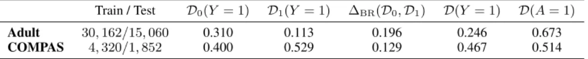
Table 1: Statistics about the Adult and COMPAS datasets.
Train / Test D0(Y = 1) D1(Y = 1) ∆BR(D0,D1) D(Y = 1) D(A= 1)
Adult 30,162/15,060 0.310 0.113 0.196 0.246 0.673
COMPAS 4,320/1,852 0.400 0.529 0.129 0.467 0.514
4.1 EXPERIMENTALSETUP
To this end, we perform experiments on two popular real-world datasets in the literature of algorithmic fairness, including an income-prediction dataset, known as theAdultdataset, from the UCI Machine Learning Repository (Dua & Graff, 2017), and the PropublicaCOMPASdataset (Dieterich et al., 2016). The basic statistics of these two datasets are listed in Table 1.
Adult Each instance in the Adult dataset describes an adult, e.g., gender, education level, age, etc, from the 1994 US Census. In this dataset we use gender as the sensitive attribute, and the processed data contains 114 attributes. The target variable (income) is also binary: 1 if≥50K/year otherwise 0. For the sensitive attributeA,A= 0means male otherwise female. From Table 1 we can see that the base rates are quite different (0.310vs.0.113) across groups in the Adult dataset. The dataset is also imbalanced in the sense that only around24.6%of the instances have target label1. Furthermore, the group ratio is also imbalanced: roughly67.3%of the data are male.
COMPAS The goal of the COMPAS dataset is binary classification on whether a criminal defendant will recidivate within two years or not. Each instance contains 12 attributes, including age, race, gender, number of prior crimes, etc. For this dataset, we use the race (whiteA= 0vs. blackA= 1) as our sensitive attribute and target variable is 1 iff recidivism. The base rates are different across groups, but the COMPAS dataset is balanced in both the target variable and the sensitive attribute.
To validate the effect of ensuring equalized odds and accuracy parity, for each dataset, we perform controlled experiments by fixing the baseline network architecture so that it is shared among all the fair representation learning methods. We term the proposed method CFAIR(for conditional
fair representations) that minimizes conditional errors both the target variable loss function and adversary loss function. To demonstrate the importance of using BER in the loss function of target variable, we compare with a variant of CFAIRthat only uses BER in the loss of adversaries, denoted as CFAIR-EO. To see the relative effect of using cross-entropy loss vsL1loss, we also show the results of LAFTR(Madras et al., 2018), a state-of-the-art method for learning fair representations. Note that LAFTRis closely related to CFAIR-EO but slightly different: LAFTRuses global cross-entropy loss for target variable, but conditionalL1loss for the adversary. Also, there is only one adversary in LAFTR, while there are two adversaries, one forD0and one forD1, in both CF
AIRand CFAIR-EO. Lastly, we also present baseline results of FAIR(Edwards & Storkey, 2015), which aims for demographic parity representations, and NODEBIAS, the baseline network without any fairness constraint. For all the fair representation learning methods, we use the gradient reversal layer (Ganin et al., 2016) to implement the gradient descent ascent (GDA) algorithm to optimize the minimax problem. All the experimental details, including network architectures, learning rates, batch sizes, etc. are provided in the appendix.
4.2 RESULTS ANDANALYSIS
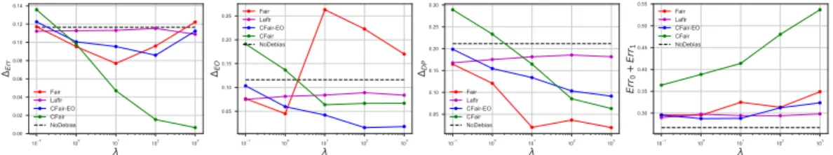
In Figure 1 and Figure 2 we show the error gap∆Err, equalized odds gap∆EO, demographic parity gap∆DPand the joint error across groupsErr0+ Err1of the aforementioned fair representation learning algorithms on both the Adult and the COMPAS datasets. For each algorithm and dataset, we also gradually increase the value of the trade-off parameterλand compute the corresponding metrics.
Figure 1: The error gap∆Err, equalized odds gap∆EO, demographic parity gap∆DPand joint error Err0+ Err1on the Adult dataset withλ∈ {0.1,1.0,10.0,100.0,1000.0}.
Figure 2: The error gap∆Err, equalized odds gap∆EO, demographic parity gap∆DPand joint error Err0+ Err1on the COMPAS dataset withλ∈ {0.1,1.0,10.0}.
Adult Due to the imbalance ofAin the Adult dataset, in the first plot of Figure 1 we can see that all the algorithms except CFAIRhave a large error gap of around 0.12. As a comparison, observe that the error gap of CFAIRwhenλ= 1e3almost reduces to 0, confirming the effectiveness of our algorithm in ensuring accuracy parity. From the second plot, we can verify that all the three methods, including CFAIR, CFAIR-EO and LAFTRsuccessfully ensure a small equalized odds gap, and they also decrease demographic parity gaps (the third plot). FAIRis the most effective one in mitigating ∆DPsince its objective function directly optimizes for that goal. Note that from the second plot we can also confirm that CFAIR-EO is more effective than LAFTRin reducing∆EO. The reason is two-fold. First, CFAIR-EO uses two distinct adversaries and hence it effectively competes with
stronger adversaries than LAFTR. Second, CFAIR-EO uses the cross-entropy loss instead of theL1 loss for the adversary, and it is well-known that the maximum-likelihood estimator (equivalent to using the cross-entropy loss) is asymptotically efficient and optimal. On the other hand, since the Adult dataset is imbalanced (in terms ofY), using BER in the loss function of the target variable can thus to a large extent hurt the utility, and this is also confirmed from the last plot, where we show the joint error.
COMPAS The first three plots of Figure 2 once again verify that CFAIRsuccessfully leads to reduced error gap, equalized odds gap and also demographic parity gap. These experimental results are consistent with our theoretical findings where we show that if the representations satisfy equalized odds, then its∆DPcannot exceed that of the optimal classifier, as shown by the horizontal dashed line in the third plot. In the fourth plot of Figure 2, we can see that as we increaseλ, all the fair representation learning algorithms sacrifice utility. However, in contrast to Figure 1, here the proposed algorithm CFAIRhas the smallest trade-off: this shows that CFAIRis particularly suited in the cases when the dataset is balanced and we would like to simultaneously ensure accuracy parity and equalized odds. As a comparison, while CFAIR-EO is still effective, it is slightly worse than CFAIRin terms of both ensuring parity and achieving small joint error.
5
RELATED
WORK
Algorithmic Fairness In the literature of algorithmic fairness, two key notions of fairness have been extensively proposed and explored, i.e.,group fairness, including various variants defined in Section 2, andindividual fairness, which means that similar individuals should be treated similarly. Due to the complexity in defining a distance metric to measure the similarity between individuals (Dwork et al., 2012), most recent research focuses on designing efficient algorithms to achieve group fairness (Zemel et al., 2013; Zafar et al., 2015; Hardt et al., 2016; Zafar et al., 2017; Madras et al., 2018; Creager et al., 2019; Madras et al., 2019). In particular, Hardt et al. (2016) proposed a post-processing technique to achieve equalized odds by taking as input the model’s prediction and the sensitive attribute. However, the post-processing technique requires access to the sensitive attribute during the inference phase, which is often not available in many real-world scenarios. Another line of work uses causal inference to define notions of causal fairness and to formulate procedures for achieving these notions (Zhang et al., 2018; Wang et al., 2019; Madras et al., 2019; Kilbertus et al., 2017; Kusner et al., 2017; Nabi & Shpitser, 2018). These approaches require making untestable assumptions. Of particular note is the observation in Coston et al. (2019) that fairness-adjustment procedures based onY in settings with treatment effects may lead to adverse outcomes. To apply our method in such settings, we would need to match conditional counterfactual distributions, which could be a direction of future research. Theoretical Results on Fairness Theoretical work studying the relationship between different kinds of fairness notions are abundant. Motivated by the controversy of the potential discriminatory bias in recidivism prediction instruments, Chouldechova (2017) showed an intrinsic incompatibility between equalized odds and predictive rate parity. In the seminal work of Kleinberg et al. (2016), the authors demonstrated that when the base rates differ between different groups, then a non-perfect classifier cannot simultaneously be statistically calibrated and satisfy equalized odds. In the context of cost-sensitive learning, Menon & Williamson (2018) show that if the optimal decision function is dissimilar to a fair decision, then the fairness constraint will not significantly harm the target utility. The idea of reducing fair classification to cost-sensitive learning is not new. Agarwal et al. (2018) explored the connection between fair classification and a sequence of cost-sensitive learning problems where each stage corresponds to solving a linear minimax saddle point problem. In a recent work (Zhao & Gordon, 2019), the authors proved a lower bound on the joint error across different groups when a classifier satisfies demographic parity. They also showed that when the decision functions are close between groups, demographic parity also implies accuracy parity. The theoretical results in this work establish a relationship between accuracy parity and equalized odds: these two fairness notions are fundamentally related by the base rate gap and the balanced error rate. Furthermore, we also show that for any predictor that satisfies equalized odds, the balanced error rate also serves as an upper bound on the joint error across demographic subgroups.
Fair Representations Through the lens of representation learning, recent advances in building fair algorithmic decision making systems focus on using adversarial methods to learn fair representations
that also preserve sufficient information for the prediction task (Edwards & Storkey, 2015; Beutel et al., 2017; Zhang et al., 2018; Madras et al., 2018; Adel et al., 2019). In a nutshell, the key idea is to frame the problem of learning fair representations as a two-player game, where the data owner is competing against an adversary. The goal of the adversary is to infer the group attribute as much as possible while the goal of the data owner is to remove information related to the group attribute and simultaneously to preserve utility-related information for accurate prediction. Apart from using adversarial classifiers to enforce group fairness, other distance metrics have also been used to learn fair representations, e.g., the maximum mean discrepancy (Louizos et al., 2015), and the Wasserstein-1 distance (Jiang et al., 2019). In contrast to these methods, in this paper we advocate for optimizing BER on both the target loss and adversary loss in order to simultaneously achieve accuracy parity and equalized odds. We also show that this leads to better utility-fairness trade-off for balanced datasets.
6
CONCLUSION AND
FUTURE
WORK
In this paper we propose a novel representation learning algorithm that aims to simultaneously ensure accuracy parity and equalized odds. The main idea underlying the design of our algorithm is to align the conditional distributions of representations (rather than marginal distributions) and use balanced error rate (i.e., the conditional error) on both the target variable and the sensitive attribute. Theoretically, we prove how these two concepts together help to ensure accuracy parity and equalized odds without impacting demographic parity, and we also show how these two can be used to give a guarantee on the joint error across different demographic subgroups. Empirically, we demonstrate on two real-world experiments that the proposed algorithm effectively leads to the desired notions of fairness, and it also leads to better utility-fairness trade-off on balanced datasets.
Calibration and Utility Our work takes a step towards better understanding the relationships between different notions of fairness and their corresponding trade-off with utility. In some scenarios, e.g., the COMPAS tool, it is desired to have a decision making system that is also well calibrated. While it is well-known that statistical calibration is not compatible with demographic parity or equalized odds, from a theoretical standpoint it is still not clear whether calibration will harm utility and if so, what is the fundamental limit of a calibrated tool on utility.
Fairness and Privacy Future work could also investigate how to make use of the close relationship between privacy and group fairness. At a colloquial level, fairness constraints require a predictor to be (to some extent) agnostic about the group membership attribute. The membership query attack in privacy asks the same question – is it possible to guarantee that even an optimal adversary cannot steal personal information through inference attacks. Prior work (Dwork et al., 2012) has described the connection between the notion of individual fairness and differential privacy. Hence it would be interesting to exploit techniques developed in the literature of privacy to develop more efficient fairness-aware learning algorithms. On the other hand, results obtained in the algorithmic fairness literature could also potentially lead to better privacy-preserving machine learning algorithms (Zhao et al., 2019).
ACKNOWLEDGMENTS
HZ and GG would like to acknowledge support from the DARPA XAI project, contract #FA87501720152 and an Nvidia GPU grant. HZ would also like to thank Richard Zemel, To-niann Pitassi, David Madras and Elliot Creager for helpful discussions during HZ’s visit to the Vector Institute.
REFERENCES
Tameem Adel, Isabel Valera, Zoubin Ghahramani, and Adrian Weller. One-network adversarial fairness. In33rd AAAI Conference on Artificial Intelligence, 2019.
Alekh Agarwal, Alina Beygelzimer, Miroslav Dudik, John Langford, and Hanna Wallach. A reductions approach to fair classification. InInternational Conference on Machine Learning, pp. 60–69, 2018.
Solon Barocas, Moritz Hardt, and Arvind Narayanan. Fairness in machine learning.NIPS Tutorial, 2017.
Shai Ben-David, Nadav Eiron, and Philip M Long. On the difficulty of approximately maximizing agreements.Journal of Computer and System Sciences, 66(3):496–514, 2003.
Alex Beutel, Jilin Chen, Zhe Zhao, and Ed H Chi. Data decisions and theoretical implications when adversarially learning fair representations.arXiv preprint arXiv:1707.00075, 2017.
Toon Calders and Sicco Verwer. Three naive bayes approaches for discrimination-free classification. Data Mining and Knowledge Discovery, 21(2):277–292, 2010.
Toon Calders, Faisal Kamiran, and Mykola Pechenizkiy. Building classifiers with independency constraints. In2009 IEEE International Conference on Data Mining Workshops, pp. 13–18. IEEE, 2009.
Alexandra Chouldechova. Fair prediction with disparate impact: A study of bias in recidivism prediction instruments.Big data, 5(2):153–163, 2017.
Alexandra Chouldechova and Aaron Roth. The frontiers of fairness in machine learning. arXiv preprint arXiv:1810.08810, 2018.
Sam Corbett-Davies and Sharad Goel. The measure and mismeasure of fairness: A critical review of fair machine learning. arXiv preprint arXiv:1808.00023, 2018.
Amanda Coston, Alexandra Chouldechova, and Edward H Kennedy. Counterfactual risk assessments, evaluation, and fairness. arXiv preprint arXiv:1909.00066, 2019.
Elliot Creager, David Madras, Joern-Henrik Jacobsen, Marissa Weis, Kevin Swersky, Toniann Pitassi, and Richard Zemel. Flexibly fair representation learning by disentanglement. InInternational Conference on Machine Learning, pp. 1436–1445, 2019.
William Dieterich, Christina Mendoza, and Tim Brennan. Compas risk scales: Demonstrating accuracy equity and predictive parity.Northpoint Inc, 2016.
Dheeru Dua and Casey Graff. UCI machine learning repository, 2017. URLhttp://archive. ics.uci.edu/ml.
Cynthia Dwork, Moritz Hardt, Toniann Pitassi, Omer Reingold, and Richard Zemel. Fairness through awareness. InProceedings of the 3rd innovations in theoretical computer science conference, pp. 214–226. ACM, 2012.
Harrison Edwards and Amos Storkey. Censoring representations with an adversary.arXiv preprint arXiv:1511.05897, 2015.
Michael Feldman, Sorelle A Friedler, John Moeller, Carlos Scheidegger, and Suresh Venkatasubra-manian. Certifying and removing disparate impact. InProceedings of the 21th ACM SIGKDD International Conference on Knowledge Discovery and Data Mining, pp. 259–268. ACM, 2015. Yaroslav Ganin, Evgeniya Ustinova, Hana Ajakan, Pascal Germain, Hugo Larochelle, François
Laviolette, Mario Marchand, and Victor Lempitsky. Domain-adversarial training of neural networks. The Journal of Machine Learning Research, 17(1):2096–2030, 2016.
Moritz Hardt, Eric Price, Nati Srebro, et al. Equality of opportunity in supervised learning. In Advances in neural information processing systems, pp. 3315–3323, 2016.
Ray Jiang, Aldo Pacchiano, Tom Stepleton, Heinrich Jiang, and Silvia Chiappa. Wasserstein fair classification.arXiv preprint arXiv:1907.12059, 2019.
James E Johndrow, Kristian Lum, et al. An algorithm for removing sensitive information: application to race-independent recidivism prediction.The Annals of Applied Statistics, 13(1):189–220, 2019. Faisal Kamiran and Toon Calders. Classifying without discriminating. In2009 2nd International
Conference on Computer, Control and Communication, pp. 1–6. IEEE, 2009.
Toshihiro Kamishima, Shotaro Akaho, and Jun Sakuma. Fairness-aware learning through regular-ization approach. In2011 IEEE 11th International Conference on Data Mining Workshops, pp. 643–650. IEEE, 2011.
Niki Kilbertus, Mateo Rojas Carulla, Giambattista Parascandolo, Moritz Hardt, Dominik Janzing, and Bernhard Schölkopf. Avoiding discrimination through causal reasoning. InAdvances in Neural Information Processing Systems, pp. 656–666, 2017.
Jon Kleinberg, Sendhil Mullainathan, and Manish Raghavan. Inherent trade-offs in the fair determi-nation of risk scores.arXiv preprint arXiv:1609.05807, 2016.
Matt J Kusner, Joshua Loftus, Chris Russell, and Ricardo Silva. Counterfactual fairness. InAdvances in Neural Information Processing Systems, pp. 4066–4076, 2017.
Christos Louizos, Kevin Swersky, Yujia Li, Max Welling, and Richard Zemel. The variational fair autoencoder.arXiv preprint arXiv:1511.00830, 2015.
David Madras, Elliot Creager, Toniann Pitassi, and Richard Zemel. Learning adversarially fair and transferable representations. InInternational Conference on Machine Learning, pp. 3381–3390, 2018.
David Madras, Elliot Creager, Toniann Pitassi, and Richard Zemel. Fairness through causal awareness: Learning causal latent-variable models for biased data. InProceedings of the Conference on Fairness, Accountability, and Transparency, pp. 349–358. ACM, 2019.
Aditya Krishna Menon and Robert C Williamson. The cost of fairness in binary classification. In Conference on Fairness, Accountability and Transparency, pp. 107–118, 2018.
Razieh Nabi and Ilya Shpitser. Fair inference on outcomes. InThirty-Second AAAI Conference on Artificial Intelligence, 2018.
Arvind Narayanan. Translation tutorial: 21 fairness definitions and their politics. InProc. Conf. Fairness Accountability Transp., New York, USA, 2018.
Yixin Wang, Dhanya Sridhar, and David M Blei. Equal opportunity and affirmative action via counterfactual predictions. arXiv preprint arXiv:1905.10870, 2019.
Muhammad Bilal Zafar, Isabel Valera, Manuel Gomez Rodriguez, and Krishna P Gummadi. Fairness constraints: Mechanisms for fair classification.arXiv preprint arXiv:1507.05259, 2015.
Muhammad Bilal Zafar, Isabel Valera, Manuel Gomez Rodriguez, and Krishna P Gummadi. Fairness beyond disparate treatment & disparate impact: Learning classification without disparate mistreat-ment. InProceedings of the 26th International Conference on World Wide Web, pp. 1171–1180. International World Wide Web Conferences Steering Committee, 2017.
Rich Zemel, Yu Wu, Kevin Swersky, Toni Pitassi, and Cynthia Dwork. Learning fair representations. InInternational Conference on Machine Learning, pp. 325–333, 2013.
Brian Hu Zhang, Blake Lemoine, and Margaret Mitchell. Mitigating unwanted biases with adversarial learning. InProceedings of the 2018 AAAI/ACM Conference on AI, Ethics, and Society, pp. 335– 340. ACM, 2018.
Han Zhao and Geoffrey J Gordon. Inherent tradeoffs in learning fair representations. InAdvances in neural information processing systems, 2019.
Han Zhao, Jianfeng Chi, Yuan Tian, and Geoffrey J Gordon. Adversarial privacy preservation under attribute inference attack.arXiv preprint arXiv:1906.07902, 2019.
A
PROOFS
A.1 PROOF OFPROPOSITION3.1
Proposition 3.1. Forg : X → Z, ifdTV(g]D0y, g]D
y
1) = 0,∀y ∈ {0,1}, then for any classifier
h:Z → {0,1},h◦gsatisfies equalized odds.
Proof. To prove this proposition, we first show that for any pair of distributionsD,D0overZand any hypothesish:Z → {0,1},dTV(h]D, h]D0)≤dTV(D,D0). Note that sincehis a hypothesis,
there are only two events in the induced probability space, i.e.,h(·) = 0orh(·) = 1. Hence by definition of the induced (pushforward) distribution, we have:
dTV(h]D, h]D0) = max E=h−1(0),orE=h−1(1)|D(E)− D 0(E)| ≤ sup Eis measurable subset ofZ |D(E)− D0(E)| =dTV(D,D0).
Apply the above inequality twice fory∈ {0,1}:
0≤dTV((h◦g)]Dy0,(h◦g)]D1y)≤dTV(g]D0y, g]D y 1) = 0, meaning dTV((h◦g)]D y 0,(h◦g)]D y 1) = 0,
which further implies thath(g(X))is independent ofAgivenY =ysinceh(g(X))is binary. A.2 PROOF OFPROPOSITION3.2
Proposition 3.2. Forg : X → Z, ifdTV(g]D y
0, g]D y
1) = 0,∀y ∈ {0,1}, then for any classifier
h:Z → {0,1},dTV((h◦g)]D0,(h◦g)]D1)≤∆BR(D0,D1). Proof. LetYb = (h◦g)(X)and note thatYb is binary, we have
dTV((h◦g)]D0,(h◦g)]D1) = 1 2 |D0(bY = 0)− D1(Yb = 0)|+|D0(Yb = 1)− D1(bY = 1)| . Now, by Proposition 3.1, ifdTV(g]D y 0, g]D y 1) = 0,∀y∈ {0,1}, it follows thatdTV((h◦g)]Dy0,(h◦ g)]D y
1) = 0,∀y∈ {0,1}as well. Applying Lemma 3.1, we know that∀y∈ {0,1},
|D0(Yb =y)− D1(Yb =y)| ≤ |D0(Y = 0)− D1(Y = 0)| · D0(Yb =y) +D1(bY =y) . Hence, dTV((h◦g)]D0,(h◦g)]D1) = 1 2 |D0(Yb = 0)− D1(bY = 0)|+|D0(Yb = 1)− D1(Yb = 1)| ≤ |D0(Y = 0)− D1(Y = 0)| 2 D0(bY = 0) +D1(bY = 0) + D0( b Y = 1) +D1( b Y = 1) = |D0(Y = 0)− D1(Y = 0)| 2 D0(bY = 0) +D0(bY = 1) + D1( b Y = 0) +D1( b Y = 1) = |D0(Y = 0)− D1(Y = 0)| 2 ·2 =|D0(Y = 0)− D1(Y = 0)| = ∆BR(D0,D1).
A.3 PROOF OFLEMMA3.1
Recall that we defineγa :=Da(Y = 0),∀a∈ {0,1}.
Lemma 3.1. Assume the conditions in Proposition 3.1 hold and letYb =h(g(X))be the classifier, then|D0(Yb =y)− D1(bY =y)| ≤ |γ0−γ1| · D0(Yb =y) +D1(Yb =y)
Proof. To bound|D0(bY =y)− D1(Yb =y)|, fory ∈ {0,1}, by the law of total probability, we have: |D0(Yb =y)− D1(Yb =y)|= = D00(bY =y)D0(Y = 0) +D01(Yb =y)D0(Y = 1) − D0 1(bY =y)D1(Y = 0) +D 1 1(Yb =y)D1(Y = 1) ≤ γ0D00(Yb =y)−γ1D01(Yb =y) + (1−γ0)D1 0(Yb =y)−(1−γ1)D11(Yb =y) ,
where the above inequality is due to the triangular inequality. Now apply Proposition 3.1, we know thatYb satisfies equalized odds, so we haveD00(Yb =y) =D10(bY =y) =D0(Yb =y)and D1 0(bY =y) =D11(bY =y) =D1(bY =y), leading to: =γ0−γ1 · D0(Yb =y) + (1−γ0)−(1−γ1)· D1(bY =y) =|γ0−γ1| · D0(Yb =y) +D1(Yb =y) ,
which completes the proof.
A.4 PROOF OFTHEOREM3.1
Theorem 3.1. Assume the conditions in Proposition 3.1 hold and letYb =h(g(X))be the classifier, then∆DP(bY)≤∆BR(D0,D1) = ∆DP(Y).
Proof. To bound∆DP(Yb), realize that|D0(Yb = 0)− D1(bY = 0)|=|D0(Yb = 1)− D1(Yb = 1)|, so we can rewrite the DP gap as follows:
∆DP(Yb) = 1 2 D0(bY = 0)− D1(Yb = 0)|+|D0(Yb = 1)− D1(Yb = 1) .
Now apply Lemma 3.1 twice fory= 0andy= 1, we have:
|D0(Yb = 0)− D1(bY = 0)| ≤ |γ0−γ1| · D0(Yb = 0) +D 1 (Yb = 0) |D0(Yb = 1)− D1(bY = 1)| ≤ |γ0−γ1| · D0(Yb = 1) +D1(Yb = 1) .
Taking sum of the above two inequalities yields
|D0(Yb = 0)− D1(Yb = 0)|+|D0(bY = 1)− D1(Yb = 1)| ≤ |γ0−γ1| D0( b Y = 0) +D1( b Y = 0) + D0( b Y = 1) +D1(bY = 1) =|γ0−γ1| D0( b Y = 0) +D0( b Y = 1) + D1( b Y = 0) +D1(bY = 1) = 2γ0−γ1 .
Combining all the inequalities above, we know that ∆DP(bY) = 1 2 D0(Yb = 0)− D1(Yb = 0)|+|D0(Yb = 1)− D1(bY = 1) ≤ γ0−γ1 =|D0(Y = 0)− D1(Y = 0)| =|D0(Y = 1)− D1(Y = 1)| = ∆BR(D0,D1) = ∆DP(Y),
completing the proof.
A.5 PROOF OFTHEOREM3.2
Theorem 3.2. Assume the conditions in Proposition 3.1 hold and letYb =h(g(X))be the classifier, thenErrD0(Yb) + ErrD1(Yb)≤2BERD(Yb ||Y).
Proof. First, by the law of total probability, we have: ErrD0(bY) + ErrD1(Yb) =D0(Y 6=Yb) +D1(Y 6=Yb)
=D1
0(Yb = 0)D0(Y = 1) +D00(Yb = 1)D0(Y = 0) +D11(Yb = 0)D1(Y = 1) +D10(Yb = 1)D1(Y = 0) Again, by Proposition 3.1, the classifier Yb = (h◦g)(X)satisfies equalized odds, so we have
D1 0(bY = 0) = D1(Yb = 0), D00(bY = 1) = D0(bY = 1), D11(Yb = 0) = D1(bY = 0) and D0 1(bY = 1) =D0(Yb = 1): =D1(Yb = 0)D0(Y = 1) +D0(Yb = 1)D0(Y = 0) +D1(Yb = 0)D1(Y = 1) +D0(Yb = 1)D1(Y = 0) =D1( b Y = 0)· D0(Y = 1) +D1(Y = 1) +D0( b Y = 1)· D0(Y = 0) +D1(Y = 0) ≤2D1( b Y = 0) + 2D0(bY = 1) = 2BERD(Yb||Y),
which completes the proof.
A.6 PROOF OFTHEOREM3.3
Theorem 3.3. For any classifierYb,∆Err(Yb)≤∆BR(D0,D1)·BERD(bY ||Y) + 2∆EO(Yb). Before we give the proof of Theorem 3.3, we first prove the following two lemmas that will be used in the following proof.
Lemma A.1. Defineγa := Da(Y = 0),∀a ∈ {0,1}, then|γ0D00(Yb = 1)−γ1D01(Yb = 1)| ≤ |γ0−γ1| · D0(Yb = 1) +γ0D0(A= 1)∆EO(Yb) +γ1D0(A= 0)∆EO(bY).
Proof. In order to prove the upper bound in the lemma, it suffices if we could give the desired upper bound for the following term
|γ0D 0 0(bY = 1)−γ1D01(Yb = 1)| − |(γ0−γ1)D0(Yb = 1)| ≤ γ0D00(Yb = 1)−γ1D10(Yb = 1) −(γ0−γ1)D0(Yb = 1) = γ0(D 0 0(bY = 1)− D0(bY = 1))−γ1(D01(bY = 1)− D0(bY = 1)) , following which we will have:
|γ0D00(Yb = 1)−γ1D10(bY = 1)| ≤ |(γ0−γ1)D0(Yb = 1)| + γ0(D 0 0(Yb = 1)− D0(Yb = 1))−γ1(D01(Yb = 1)− D0(bY = 1)) , and an application of the Bayes formula could finish the proof. To do so, let us first simplify D0
0(bY = 1)− D0(bY = 1). Applying the Bayes’s formula, we know that: D0 0(Yb = 1)− D0(Yb = 1) =D00(Yb = 1)− D00(bY = 1)D0(A= 0) +D10(bY = 1)D0(A= 1) = D00(bY = 1)− D 0 0(bY = 1)D 0(A= 0) − D10(Yb = 1)D0(A= 1) =D0(A= 1) D0 0(bY = 1)− D 0 1(bY = 1) .
Similarly, for the second termD0
1(Yb = 1)− D0(Yb = 1), we can show that: D0 1(bY = 1)− D 0(bY = 1) =D0(A= 0) D0 1(Yb = 1)− D00(Yb = 1) .
Plug these two identities into above, we can continue the analysis with γ0(D 0 0(bY = 1)− D0(bY = 1))−γ1(D01(bY = 1)− D0(bY = 1)) = γ0D 0(A= 1)( D00(Yb = 1)− D01(Yb = 1))−γ1D0(A= 0)(D01(Yb = 1)− D00(bY = 1)) ≤ γ0D 0(A= 1)(D0 0(Yb = 1)− D01(Yb = 1)) + γ1D 0(A= 0)(D0 1(Yb = 1)− D00(bY = 1)) ≤γ0D0(A= 1)∆EO(Yb) +γ1D0(A= 0)∆EO(bY).
The first inequality holds by triangular inequality and the second one holds by the definition of
Lemma A.2. Defineγa:=Da(Y = 0),∀a∈ {0,1}, then|(1−γ0)D01(bY = 0)−(1−γ1)D11(Yb = 0)| ≤ |γ0−γ1| · D1(Yb = 0) + (1−γ0)D1(A= 1)∆EO(bY) + (1−γ1)D1(A= 0)∆EO(bY). Proof. The proof of this lemma is symmetric to the previous one, so we omit it here. Now we are ready to prove Theorem 3.3:
Proof of Theorem 3.3. First, by the law of total probability, it is easy to verify that following identity holds fora∈ {0,1}:
Da(bY 6=Y) =Da(Y = 1,Yb = 0) +Da(Y = 0,Yb = 1) = (1−γa)D1a(Yb = 0) +γaD0a(Yb = 1). Using this identity, to bound the error gap, we have:
|D0(Y 6=Yb)− D1(Y 6=Yb)|= ((1−γ0)D01(Yb = 0) +γ0D00(bY = 1))−((1−γ1)D 1 1(Yb = 0) +γ1D10(Yb = 1)) ≤ γ0D00(Yb = 1)−γ1D10(Yb = 1) + (1−γ0)D10(Yb = 0)−(1−γ1)D11(bY = 0) . Invoke Lemma A.1 and Lemma A.2 to bound the above two terms:
|D0(Y 6=Yb)− D1(Y 6=Yb)| ≤ γ0D00(Yb = 1)−γ1D10(Yb = 1) + (1−γ0)D10(Yb = 0)−(1−γ1)D11(bY = 0) ≤γ0D0(A= 1)∆EO(bY) +γ1D0(A= 0)∆EO(Yb) + (1−γ0)D1(A= 1)∆EO(Yb) + (1−γ1)D 1 (A= 0)∆EO(Yb) +γ0−γ1 D0(Yb = 1) + γ0−γ1 D1(Yb = 0), Realize that bothγ0, γ1∈[0,1], we have:
≤ D0(A= 1)∆EO(Yb) +D0(A= 0)∆EO(Yb) +D1(A= 1)∆EO(Yb) +D1(A= 0)∆EO(bY) +γ0−γ1 D0(Yb = 1) + γ0−γ1 D1(Yb = 0) = 2∆EO(bY) +γ0−γ1 D0(Yb = 1) + γ0−γ1 D1(Yb = 0) = 2∆EO(bY) + ∆BR(D0,D1)·BERD(Yb ||Y),
which completes the proof.
We also provide the proof of Corollary 3.1:
Corollary 3.1. For any joint distributionDand classifierYb, ifYb satisfies equalized odds, then max{ErrD0(Yb),ErrD1(Yb)} ≤∆BR(D0,D1)·BERD(Yb ||Y)/2 + BERD(bY ||Y).
Proof. We first invoke Theorem 3.3, ifYb satisfies equalized odds, then∆EO(Yb) = 0, which implies: ∆Err(Yb) =
ErrD0(bY)−ErrD1(Yb)
≤∆BR(D0,D1)·BERD(bY ||Y). On the other hand, by Theorem 3.2, we know that
ErrD0(bY) + ErrD1(Yb)≤2BERD(bY ||Y).
Combine the above two inequalities and recall thatmax{a, b}= (|a+b|+|a−b|)/2,∀a, b∈R,
yielding:
max{ErrD0(bY),ErrD1(bY)}=
|ErrD0(Yb)−ErrD1(Yb)|+|ErrD0(Yb) + ErrD1(bY)|
2
≤ ∆BR(D0,D1)·BERD(Yb ||Y) + 2BERD(bY ||Y) 2
= ∆BR(D0,D1)·BERD(bY ||Y)/2 + BERD(Yb ||Y),
B
EXPERIMENTAL
DETAILS
B.1 THEADULTEXPERIMENTFor the baseline network NODEBIAS, we implement a three-layer neural network with ReLU as the hidden activation function and logistic regression as the target output function. The input layer contains 114 units, and the hidden layer contains 60 hidden units. The output layer only contain one unit, whose output is interpreted as the probability ofD(Yb = 1|X =x).
For the adversary in FAIRand LAFTR, again, we use a three-layer feed-forward network. Specifically, the input layer of the adversary is the hidden representations of the baseline network that contains 60 units. The hidden layer of the adversary network contains 50 units, with ReLU activation. Finally, the output of the adversary also contains one unit, representing the adversary’s inference probability D(Ab= 1|Z =z). The network structure of the adversaries in both CFAIRand CFAIR-EO are exactly the same as the one used in FAIRand LAFTR, except that there are two adversaries, one for D0(
b
A= 1|Z=z)and one forD1( b
A= 1|Z =z).
The hyperparameters used in the experiment are listed in Table 2.
Table 2: Hyperparameters used in the Adult experiment.
Optimization Algorithm AdaDelta
Learning Rate 1.0
Batch Size 512
Training Epochsλ∈ {0.1,1.0,10.0,100.0,1000.0} 100
B.2 THECOMPAS EXPERIMENT
Again, for the baseline network NODEBIAS, we implement a three-layer neural network with ReLU as the hidden activation function and logistic regression as the target output function. The input layer contains 11 units, and the hidden layer contains 10 hidden units. The output layer only contain one unit, whose output is interpreted as the probability ofD(Yb = 1|X =x).
For the adversary in FAIRand LAFTR, again, we use a three-layer feed-forward network. Specifically, the input layer of the adversary is the hidden representations of the baseline network that contains 60 units. The hidden layer of the adversary network contains 10 units, with ReLU activation. Finally, the output of the adversary also contains one unit, representing the adversary’s inference probability D(Ab= 1|Z =z). The network structure of the adversaries in both CFAIRand CFAIR-EO are exactly the same as the one used in FAIRand LAFTR, except that there are two adversaries, one for D0(
b
A= 1|Z=z)and one forD1( b
A= 1|Z =z).
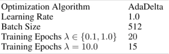
The hyperparameters used in the experiment are listed in Table 3.
Table 3: Hyperparameters used in the COMPAS experiment. Optimization Algorithm AdaDelta
Learning Rate 1.0
Batch Size 512
Training Epochsλ∈ {0.1,1.0} 20 Training Epochsλ= 10.0 15