Grey-Level Co-occurrence features for salt texture classification

Grey-Level Co-occurrence

features for salt texture

classification

Igor Orlov

Grey-Level Co-occurrence features for salt

texture classification

Igor Orlov

Institutt for informatikk, University of Oslo Ole Johan Dahls Hus

Gaustadalléen 23 B N-0373 OSLO

Norge [email protected] 7th December 2015

Abstract

Salt structures form only two percent of world’s sedimentary rocks, but cover about half of the largest oilfields. Thus, exploration and detection of salt tectonics is very interesting for oil and gas industry.

Seismic imaging in a common method to search for salt structures in the crust. Due to the increasing volume of seismic data, and the necessity of classifying this data, as well as the complexity of the segmentation of salt structures in the seismic images, there is a strong demand for an image processing system for computer-aided salt texture detection and segmen-tation. The difficulty of salt texture segmentation in these images is that an accurate velocity model is needed. The velocity of salt is very high so to get a good quality image of the salt iterative imaging is needed. Based on a segmentation of the salt, the seismic data is reprocessed and new velocity estimates can be computed in an iterative manner. For the analysis a subset of marine seismic images from the North Sea was used.

In this thesis the differences between sediment rock and salt diapir textures are discussed, and texture features are used to classify the seismic image pixels into one of two classes. Gray level co-occurrence matrices (GLCM) is a widely used statistical texture descriptor in a local window surround-ing each pixel. To analyze the textures, we use the comparison of differ-ent GLCM-features to check which of them helps to separate two texture classes with the best performance. In addition, a new feature based on the calculation of the Mahalanobis distance between the average GLCMs for two classes was introduced. This feature has shown better classification re-sults than standard GLCM features on a set of test images and can be used for salt texture segmentation in combination with other known features such as statistical, texture or features based on digital signal processing.

Acknowledgments

The entire research for this thesis was led by my supervisor, Anne H Schis-tad Solberg. I would like to thank her for all the help, advices, scientific sources and goals she set for me during this semester. Without her kind help and patience, this thesis would never be written.

I would also like to thank my wife Nastya and my family for support and motivation.

Thank you! Igor Orlov December 2015

Contents

I Introduction and Background 1

1 Introduction 3

1.1 Marine seismic images . . . 3

1.1.1 Seismic images acquisition and pre-processing . . . . 3

1.1.2 Salt structures in seismic images . . . 3

1.2 Motivation and problem statement . . . 4

1.3 Structure of the thesis . . . 5

2 Background 7 2.1 Textures in North Sea seismic images . . . 7

2.2 Texture description methods . . . 9

2.2.1 Gray level co-occurrence matrices . . . 10

2.2.2 GLCM features . . . 11

2.2.3 Other texture analysis methods . . . 12

2.3 Distance metrics used for classification . . . 12

2.4 Gaussian classifier . . . 13

II Implementation and Evaluation 17 3 Implementation 19 3.1 Input image and mask . . . 19

3.2 Finding the optimal GLCM parameters . . . 19

3.3 Mahalanobis distance matrix . . . 23

4 Evaluation 31 4.1 Training a Gaussian classifier . . . 31

4.2 Classification results . . . 31

4.2.1 Classification results on the training data set . . . 31

4.2.2 Classification results on training and test images . . . 32

5 Summary and Conclusion 39 5.1 Thesis results . . . 39

5.1.1 Covered theoretical background . . . 39

5.1.2 Achieved results . . . 39

5.2 Further work . . . 40

List of Figures

1.1 a) Diagram for marine seismic acquisition in 2D (zigzag.co.za, 2013) and b) Schematics of the receiver array for marine seis-mic acquisition in 2D (subseaworldnews.com, 2015) . . . 4 1.2 Sedimentary basins with an intensive salt tectonics shown in

white (Geophysics journal, Kiev, 2013) . . . 4 1.3 Salt dome trap (Long Island University, 2007) . . . 5 2.1 Schematics of seismic textures for a) inline and b) timeslice

sections (Berthelot et al., 2013, [2]) . . . 8 2.2 a) An inline and b) timeslice from a North Sea dataset . . . . 8 2.3 Inline section with the color masks corresponding to the four

classes: sub-horizontal reflectors (yellow), up-dipping re-flectors (light orange), salt (blue) and down-dipping reflec-tors (dark orange) [2]. . . 9 2.4 Timeslice with the color masks corresponding to the three

classes: salt (blue), sub-horizontal reflectors (yellow) and steep dipping reflectors (orange) [2]. . . 10 2.5 Schematics for GLCM in local window of size 7, for d = 1

andθ =0 . . . 11

2.6 Model of Gaussian classifier in two-dimensional case ("Pat-tern recognition", Duda and Hart, 2001, [6]) . . . 14 3.1 Input training data: a) inline slice and b) mask. . . 20 3.2 Histogram of input image a) before and b) after cutting

histogram tails. . . 20 3.3 a) Original inline image and b) normalized after applying a

mask. . . 20 3.4 Distance matrices plots in horizontal direction by distance,

window 51x51. . . 24 3.5 Distance matrices plots in diagonal 45°direction by distance,

window 51x51. . . 25 3.6 Distance matrices plots in vertical direction by distance,

window 51x51. . . 26 3.7 Distance matrices plots in isotropic direction by distance,

window 51x51. . . 27 3.8 Plot of Mahalanobis distance between two classes

3.9 Plot of Mahalanobis distance between two classes

depend-ing on direction and offset for window size 51x51. . . 28

3.10 Distance matrix for isotropic direction and offset 2, window size 51, seen from two viewpoints. . . 29

4.1 Example of inline section with manually interpreted salt borders. . . 33

4.2 Original inline image used for training and evaluation (normalized). . . 34

4.3 Original inline image classification by variance. . . 34

4.4 Original inline image classification by Contrast. . . 35

4.5 Original inline image classification by Energy. . . 35

4.6 Original inline image classification by Correlation. . . 35

4.7 Original inline image classification by Homogeneity. . . 36

4.8 Original inline image classification by Distance. . . 36

4.9 Original inline image classification by Energy and Distance. 36 4.10 Original inline image classification by Energy and Variance. 37 4.11 Original inline image classification by Energy, Distance and Variance. Overtraining due to singularity in features. . . 37

4.12 Original inline image classification by Contrast, Energy and Distance. Correlation is present in features. . . 37

4.13 Original inline image classification by Contrast, Distance and Weighted Energy. Visually the best result. . . 38

4.14 Test inline image (inlinekorr700) classification by Contrast, Distance and Weighted Energy. . . 38

List of Tables

4.1 Comparison of classification results for classifier trained on one feature . . . 32 4.2 Comparison of classification results for classifier trained on

Listings

2.1 Pseudo-code for Gaussian classifier for n . . . 15

3.1 Matlab code for computing the distance GLCM . . . 22

A.1 Computing GLCM features for classification . . . 43

Part I

Chapter 1

Introduction

In this chapter we briefly describe how the marine seismic images used in the thesis were obtained and velocity model that is used for their formation. Also, we provide the motivation and problem statement for this thesis.

1.1

Marine seismic images

1.1.1 Seismic images acquisition and pre-processing

Seismic imaging is among the most popular geophysical methods used in the oil and gas industry for carbohydrates exploration. It is a non-destructive method to obtain a 3D image of a marine subsurface. Air guns, connected to survey vessels, shoot an air bunch and form a pressure, travel-ling downwards as a sound wave. These volume waves are reflected from discontinuities where the physical properties of a subsurface change. Re-flected waves are recorded by an array of receivers, either 2D (figure 1.1a) or 3D (figure 1.1b).

Seismic wave recording, obtained by a seismic receiver corresponding to one point of the surface with a fixed oscillation source is calledseismic trace. In fact, the seismic trace is the dependence of the amplitude of recorded waves from time, basically, A (t). The amplitudes of recorded traces cor-respond to the changes in acoustic impedance associated with sedimen-tary rock layers in the crust. These amplitude variations, as a function of time and receiver position, give an image of a subsurface seismic structure. These time recordings are processed in large-scale computers to reconstruct a model of the subsurface, i.e. of the arrangements of the rock layers accu-mulated and deformed within the different geological periods [2].

1.1.2 Salt structures in seismic images

After receiving and pre-processing the input time recordings, the main step consists in mapping the time of the primary reflections into the reflectors of known depth. This mapping is called prestack migration and requires an accurate velocity model [2]. The initial velocity model is based on

(a) (b)

Figure 1.1: a) Diagram for marine seismic acquisition in 2D (zigzag.co.za, 2013) and b) Schematics of the receiver array for marine seismic acquisition in 2D (subseaworldnews.com, 2015)

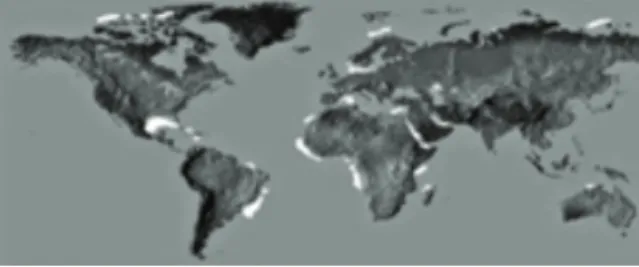
Figure 1.2: Sedimentary basins with an intensive salt tectonics shown in white (Geophysics journal, Kiev, 2013)

manual mapping of image textures to classes, and after that is iteratively updated. In the areas of complex geology such as salt, it is hard to build a velocity model. This process usually needs geologists to manually interpret different geological layers, and is known to be one of the most labour intensive tasks.

1.2

Motivation and problem statement

Salt-bearing sedimentary basins are distributed throughout the world, as demonstrated in figure 1.2. Many large hydrocarbon fields in these basins are often associated with salt structures [18]. Salt tectonics produces a vari-ety of tectonic, structural, stratigraphic and combined conditions for trap-ping hydrocarbons (1.3). Thus, detection and segmentation of salt struc-tures in seismic images is a task of great interest for oil and gas industry. Delimiting the boundary of salt structures is a challenging and important task for iterative imaging of oil reservoirs. To get a good seismic image, a velocity estimate is needed, and to get this velocity estimate correct, an initial segmentation of the boundary of the salt structure is needed. This is often interpreted manually, and is a time-consuming task, so an automatic segmentation of salt structures will be very valuable. Texture attributes is a well-known and tested (e.g. [2], [3], [17]) way for efficient salt texture

Figure 1.3: Salt dome trap (Long Island University, 2007)

mentation. Gray level co-occurence matrices and their features ([11], [1]) is a widely used texture description tool, that gives good enough results in this task.

This thesis has two main tasks:

• Provide an algorithm and visualization tool for finding the optimal GLCM parameters (in the context of salt segmentation), such as direction, offset and window size.

• Check whether distance matrix between two classes can serve as a new GLCM feature for salt segmentation, and how good is its performance comparing to widely used GLCM features.

1.3

Structure of the thesis

This thesis has the following structure in order to, first, present the ideas for methods used for research and provide a theoretical background for these methods, and then to describe the implementation details and performance evaluation.

In the introduction chapter we presented how the marine seismic im-ages are formed, and how the salt structures look like on these imim-ages. In addition, motivation and goals for the thesis were stated. In the second chapter, Background, we describe the methods used in the research, cov-ering some implementation and performance details and giving references to other possible solutions for a task of salt texture segmentation.

Second part called Implementation and Evaluation. Chapter Implementa-tion first presents the input dataset from North Sea, then describes in details

the algorithms used for visualization and hypothesis testing in this research project, covers their Matlab implementation and performance. Chapter Evaluation provides results together with figures, tables and charts for above mentioned algorithms, describes and analyzes whether presented feature can be used for salt texture segmentation.

The final chapter summarizes the thesis, discusses whether the tasks were achieved or not and what are the possible ways for further research in this area.

Chapter 2

Background

In this chapter we will provide the theoretical background for the methods used in the next chapters for texture description, classification and segmentation. First, we cover the differences between textures of salt structures and other sediments in marine seismic images from North Sea dataset. Then, we present some of the texture description methods, mostly focusing on the GLCMs as they were the main feature extraction method in this thesis. We will shortly cover possible distance metrics used in pattern recognition. In the last part of the chapter we explain the concept of Gaussian classification used for GLCM features performance evaluation.

2.1

Textures in North Sea seismic images

This thesis analyzes whether a texture-based segmentation can be used for salt texture detection in marine seismic images. We have to admit, that only a single 3D input dataset from the North Sea Central graben has been in-vestigated. This is due to the limited access to seismic data. However, the task was to test the hypothesis and provide an algorithm that will work for the input data, with some degree of generalization to expect that it will also work on seismic image datasets from other regions.

Despite the fact that original data is stored in a 3D form, we only use 2D images to do texture interpretation in the context of salt. 3D analysis in-cluding extension of GLCM texture features to three-dimensional case can be a further research outside the scope of current thesis. A given 3D sub-cube can be cut into multiple inline (vertical) or timeslice (horizontal) sec-tions (figure 2.1). We were studying only inline secsec-tions due to the clear parallel and sub-parallel pattern in textures corresponding to sedimentary rocks, and clear upward- and downward-dipping texture regions close to the salt diapir.

There are various definitions of a texture present in the image processing literature. Most of them consider an image as a patchwork, where each patch corresponds to one texture with its own parameters, such as similar-ity, contrast and orientation, that make it visually separable from the other

(a)

(b)

Figure 2.1: Schematics of seismic textures for a) inline and b) timeslice sections (Berthelot et al., 2013, [2])

(a)

(b)

Figure 2.2: a) An inline and b) timeslice from a North Sea dataset

parts of an image. Texture distributions can be random or periodic, but most of the real world examples are a mix of both. Classification of texture types in seismic images can be found in Schlaf et al. ([14]).

The examples of inline and timeslice sections from a North Sea 3D dataset corresponding to schematics in figure 2.1 are shown in figure 2.2. The ma-rine seismic textures can be divided into three groups: salt, steep-dipping reflectors and sub-horizontal reflectors (Berthelot, 2013, [2]).

Salt. Texture inside the salt is mostly characterized as an incoherent, low amplitude area with small variance both for inline and timeslice sections [2]. Salt is shown in blue masks on figures 2.3 and 2.4). Salt texture is the object of segmentation in chapter 3 Implementation and is of the most in-terest for this thesis.

Figure 2.3: Inline section with the color masks corresponding to the four classes: sub-horizontal reflectors (yellow), up-dipping reflectors (light orange), salt (blue) and down-dipping reflectors (dark orange) [2].

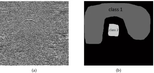
Sub-horizontal reflectorsmostly correspond to sedimentary rocks. On in-line slices, they appear to have a pseudo periodic, high frequency layer-ing structure along the horizontal direction (yellow masks on figure 2.3). For timeslices, they are no longer high frequency and pseudo periodic, but heavily vary in spatial frequencies and orientations (yellow masks in fig-ure 2.4). Sub-horizontal reflectors correspond to the class 1 from the input inline mask shown in figure 3.1b.

Steep-dipping reflectorshave the vertical, pseudo periodic and high fre-quency texture in case of inline slices (light orange and dark orange masks on figure 2.3). In case of timeslices (orange masks in figure 2.4), they have the same dip independent of the direction and appear as circle-like curves surrounding the salt [2]. Training mask with two classes presented in chap-ter Implementation, contained mostly salt and sub-horizontal reflectors, with a small regions of steep-dipping reflectors in class 1.

2.2

Texture description methods

One of the most widely used texture description methods is statistical texture analysis. In this method, texture features are computed from the statistical distribution of observed combinations of intensities at specified positions relative to each other in the image [1], usually in a square local window of odd size. According to the number of intensity points (pixels) in each combination, statistics are classified into first-order, second-order and higher-second-order statistics. First second-order statistics are, for example, mean, variance and higher order moments. They are easy to compute and variance, for example, can be used in the task of salt structures segmentation in combination with more advanced features [2]. However, they only take into account global texture parameters ("roughness" in case of variance), and not mutual intensity distribution between pixels. Second

Figure 2.4: Timeslice with the color masks corresponding to the three classes: salt (blue), sub-horizontal reflectors (yellow) and steep dipping reflectors (orange) [2].

order statistical texture features are called gray level co-occurrence matrices (GLCMs) and were first presented by Haralick et al. [11], [10].

2.2.1 Gray level co-occurrence matrices

A GLCM is a matrix where the number of rows and columns is equal to the number of gray levels, G, in the image. The matrix element P(i,j |∆x,∆y) is the relative frequency with which two pixels, separated by a pixel distance (∆x,∆y), occur within a given neighborhood, one with intensity i and the other with intensity j [1]. One may also say that the matrix element P(i, j | d,∆) contains the second order statistical probability values for changes between gray levels i and j at a particular displacement distance d and at a particular angle (θ).

Formal GLCM definition is provided in equations 2.1 to 2.4. Given M×N image with G gray levels, and f(m,n) is the intensity, GLCM is matrix P of size G×G.

P(i,j|∆x,∆y) =WQ(i,j|∆x,∆y) (2.1)

W = 1

(M−_∆x)(N−_∆y) (2.2)

Figure 2.5: Schematics for GLCM in local window of size 7, ford = 1 and θ =0 Q(i,j|_∆x,∆y) = N−∆y

∑

∑

The less formal definition might be stated as follows. For each pixel of the image we getw×wlocal window surrounding it. The dimension of GLCM isG×G, where G is number of gray levels in the image. For offsetdand directionθ loop through all pixel pairs with distance dand directionθ in

the local window (figure 2.5). Q(i,j|d,θ)is the number of pixel pairs where

pixel 1 in the pair has pixel value iand pixel 2 has pixel valuej. NB: We used 16 gray levels for all GLCMs in the current research project.

GLCMs are usually calculated in four directions - horizontal (0°), verti-cal (90°) and two diagonal (45°and 135°). Direction independent GLCM is called isotropic and computed by averaging GLCMs for all four direc-tions. GLCM for direction 180°is a transposed GLCM for 0°, so they are usually summed up and GLCMs are symmetric with respect to diagonal.

2.2.2 GLCM features

There are many features that can be extracted from the GLCM. Usually they measure the homogeneity or the contrast in the local window. Some of them were presented in the original paper [11], while others have been invented later [7], [19], [5]. In our thesis we tried to invent our own GLCM feature based on Mahalanobis distance between average GLCMs for two classes, and compared to several standard GLCM features that Matlab sup-ports out-of-the-box in function graycoprops, such as Contrast (equation 2.5), Correlation (2.6), Energy (2.7) and Homogeneity (2.8).

Contrast=

∑

i,j

Correlation=

∑

∑

∑

∑

∑

2.2.3 Other texture analysis methods

There are also other analysis methods used in salt texture segmentation problems, such as Gabor filters [16], normalized cut segmentation [12], lo-cal Fourier spectra [17] and dip and frequency attributes [8]. They have not been used in a research, however, they can be good candidates for a com-bination with some of the GLCM features described above. Variance in a local window has also been tested as a texture attribute in Matlab imple-mentation, see chapter 3.

2.3

Distance metrics used for classification

To compute the distance matrix between average GLCMs for two input classes from an input mask (see chapter Implementation), we used a Ma-halanobis distance [13]. Unlike Euclidean distance (2.9), that does not take into account in-class distribution of vectors p and q, Mahalanobis distance measures the number of standard deviations from p to the mean of d. If each of these axes is rescaled to have unit variance, then Mahalanobis dis-tance equals to standard Euclidean disdis-tance in the transformed space. Ma-halanobis distance is thus unitless and scale-invariant, and takes into ac-count the correlations of the data set [9]. In case of two classes, we calculate Mahalanobis distance between mean values in these two classes (average GLCMs),Σis computed as an average ofΣ1andΣ22.10.

deucl(p,q) = q (p1−q1)2+ (p2−q2)2+. . .+ (pi−qi)2+. . . (2.9) dmahal(p,q) = q (p−q)tΣ−1_{(p−q) (2.10)}

Another possible statistical distance to use was Bhattacharyya distance [4]. It measures the separability of classes in classification and it is considered

to be more reliable than the Mahalanobis distance, as the latter is a partic-ular case of the former when the standard deviations of the two classes are the same. The Bhattacharyya coefficient is an approximate measurement of the amount of overlap between two statistical samples, and can be used to determine the relative closeness of the two samples being considered 2.11. However, only Mahalanobis distance was used for current research.

BC(p,q) = n

∑

2.4

Gaussian classifier

In order to estimate and compare the performance of existing GLCM fea-tures for salt segmentation with our own distance feature, we need to choose a classifier, train it on some training set (mask for salt and sediments is described in section 3.1) and test classifier performance on a training set, then on entire inline image and on other inline images from the dataset. We needed a very basic classifier, because the main goal was not to esti-mate the classifier performance, but the texture features performance. We picked multivariate Gaussian classifier due to its simplicity and training speed, and current section describes the basic idea behind this method and implementation in Matlab. More detailed theoretical description can be found in [6] and [15]. We can expect that choosing more advanced classifier such as SVM, neural networks etc. might increase the overall segmentation performance for given features and parameters, but this task is outside of the main goal of this thesis.

Gaussian classifieris a simple probabilistic classifier based on Bayes’ rule. A typical assumption for Gaussian classifier is that the continuous values associated with each class are distributed according to a Gaussian distribu-tion.

Suppose we have J, j=1,..,J classes. wj is the class label for a pixel, andxis

the observed feature vector [15]. We can use Bayes rule to find an expres-sion for the class with the highest probability (equation 2.12). P(wj) is the

prior probability for classwj. If we don’t have special knowledge that one

of the classes occurs more frequent than other classes, we set them equal for all classes (P(wj)=1/J, j=1,..,J). In this thesis we also used equal probabilities,

as the proportion in the training data is normally not representative.

P(w_j|x) =P(w_j)P(x|wj)

P(x) (2.12)

posterior= prior×likelihood

normalization f actor (2.13)

In formula 2.12 p(x|wj) is the probability density function that models the

Figure 2.6: Model of Gaussian classifier in two-dimensional case ("Pattern recognition", Duda and Hart, 2001, [6])

In case of a Gaussian classifier we assume that the distribution is Gaussian and the mean and covariance of that distribution are fitted to some data that we know belongs to class (refer to [15]). This data is called training data and this fitting is called the classifier training. P(wj|x) is the posterior

probability that pixelxactually belongs to classw_j. p(x) is a scaling factor that assures that the probabilities sum is equal to 1 (equation 2.13). The general form for multivariate Gaussian density function is shown in 2.14, whereµsis a 1×nmean vector for training vectors for class S, andΣs- is a

n×ncovariance matrix, where elementσijis a covariance between features

i and j in training vectors for class S, andnis a number of features.

P(x|ws) =

1

p

|Σs|(2π)n/2

e−12(x−µs)tΣs−1(x−µs) _(2.14)

In the two-dimensional case, the Gaussian model can be thought of as an approximation of the classes in 2D feature space with ellipses. The mean vectorµ = [µ1,µ2]defines the center point of the ellipses. σ12, the

covari-ance between the features defines the orientation of the ellipse.σ11andσ22,

define the width of the ellipse (the a and b parameters). The Mahalanobis distance between a given pointxand the class centerµis shown in equation

2.15. Schematics of Gaussian classifier in two-dimensional case (as ellipse) is shown in figure 2.6.

r2= (x−µ)TΣ−1(x−µ) (2.15)

Listing 2.1 provides a pseudo-code for Matlab implementation of Gaussian classifier used in the next chapters.

Listing 2.1: Pseudo-code for Gaussian classifier for n

p r o b a b i l i t y 1 = count1 / ( count1 + count2 ) ;

% same f o r p r o b a b i l i t y 2 . . .

% mean1 − mean o f a l l f e a t u r e v e c t o r s f r o m c l a s s 1 % c o v a r M a t r 1 − c o v a r i a n c e m a t r i x .

% same f o r mean2 and c o v a r M a t r 2 . . .

r e s u l t 1 = p r o b a b i l i t y 1 * exp(−_{0 . 5 *( x}−_{mean1 ) * . . .}

inv_{( covarMatr1 ) * ( x}−_{mean1 ) ’ ) / ( 2 *}pi_*s q r t(det( covarMatr1 ) ) ) ;

% same f o r r e s u l t 2 . . . i f r e s u l t 1 > r e s u l t 2 % x b e l o n g s t o c l a s s 1 e l s e % x b e l o n g s t o c l a s s 2 end

Part II

Implementation and

Evaluation

Chapter 3

Implementation

The goal of the project is, first, to find the optimal GLCM parameters (win-dow size, direction and offset) in terms of separation between two input classes for sedimentary rocks and for salt. And second, to investigate which GLCM feature is most efficient for salt texture segmentation in seismic im-ages and compare results with segmentation by our own feature, based on Mahalanobis distance between class means. This chapter describes the training data from the North Sea dataset and implementation details for finding the optimal GLCM feature, visualization of average GLCMs, calcu-lation of Mahalanobis distance, classification etc.

3.1

Input image and mask

The input training image is an inline slice from the North Sea 3D dataset of size 1401x1501 with values in range from -346.8 to 399.1 (figure 3.1a). In ad-dition, a pixel mask for this image was provided (pixel value 1 corresponds to class 1 - sub-horizontal reflectors, value 2 to salt structures, and 0 - other not mapped pixels). Input mask is shown in figure 3.1b. There are totally 830729 pixels of class 1 (sedimentary rocks) and 57253 pixels of class 2 (salt). Pprocessing has to be very basic to keep the algorithm and research re-sults general. Only histogram tails were cut to range [-100;+100] (figure 3.2) and then image was normalized - shifted to the range [0;255]. Neither histogram equalization nor any other technique were applied.

Figure 3.3 shows mask on top of the original (3.3a) and normalized (3.3b) inline input image.

3.2

Finding the optimal GLCM parameters

The first task was to find the GLCM parameters (direction, offset, window size) that help to separate between pixels of two given classes in an optimal way. Optioptimal in terms of maximizing the norm of a distance matrix

-(a) (b)

Figure 3.1: Input training data: a) inline slice and b) mask.

Figure 3.2: Histogram of input image a) before and b) after cutting histogram tails.

(a) (b)

Figure 3.3: a) Original inline image and b) normalized after applying a mask.

pixel-wise Mahalanobis distance between the average GLCM of class 1 and average GLCM of class 2.

For each pixel from class 1 or 2, for the chosen GLCM parameters and 16 gray levels, we can compute a corresponding GLCM that can be seen as a feature vector of size 16×16=256. Then, we find the mean values for two classes (calculating a mean for each of 256 elements) and then, again, for all elements, we calculate a Mahalanobis distance between the classes. This distance vector of size 1x256 can be converted to a distance matrix of size 16x16, that, basically, represents a distance between average GLCMs for pixels from class 1 and 2. This matrix shows which of the GLCM elements are the most different between these two classes and, thus, can be used as a weighing window to improve the classification or as a GLCM feature itself. The greater the norm of this matrix, the better separation is provided by the chosen GLCM parameters.

The following parameters were used and tested in the experiment: • 16 gray levels, fixed (i.e. all GLCMs had size 16x16);

• local windows sizes - 31x31 and 51x51;

• GLCM directions - horizontal (0°), vertical (90°), diagonal (45°and 135°) and isotropic (average in all 4 directions), see subsection 2.2.1; • GLCM offset from 1 to 15 pixels for 31x31, 1 to 20 pixels for 51x51. Here is a description of the algorithm used to calculate the distance matrix between average GLCMs for two classes:

1. Find pixel coordinates for all pixels from classes 1 and 2 2. Pick GLCM parameters - window size (31 or 51) and direction; 3. For every offset from 1 to 20 do:

(a) For every pixel from class 1 calculate a GLCM matrix, and calculate an average GLCM matrix for class 1, and standard deviation for each of 256 matrix elements;

(b) Do the same for class 2

(c) Create a new 16x16 matrix where element (i,j) is Mahalanobis distance between (i,j) element of average GLCM for class 1 and same of class 2, standard deviation isstdi,j = std1i,j

+std2i,j

2

4. Calculate the norm of a distance matrix.

The following listing demonstrates the main parts of Matlab implementa-tion for the above described algorithm.

Listing 3.1: Matlab code for computing the distance GLCM % l o a d i n l i n e i m a g e and mask % Cut h i s t o g r a m t a i l s and s h i f t t o 0 . . 2 5 5 downLimit = −100; upLimit = 1 0 0 ; i n l i n e I m g ( i n l i n e I m g < downLimit ) = downLimit ; i n l i n e I m g ( i n l i n e I m g > upLimit ) = upLimit ; i n l i n e I m g = normalize2D ( i n l i n e I m g ) ; % C h o o s e GLCM p a r a m e t e r s g r a y L e v e l s = 1 6 ; halfWin = 2 5 ; distanceMax = 2 0 ; % F i n d e l e m e n t s i f c l a s s 1 and 2 [ c l a s s 1 _ X , c l a s s 1 _ Y ] = find( maskImg = = 1 ) ; [ c l a s s 2 _ X , c l a s s 2 _ Y ] = find( maskImg = = 2 ) ; % F o r d i s t a n c e f r o m 1 t o d i s t a n c e M a x % and d i r e c t i o n , c a l c u l a t e a v e r a g e GLCMs f o r d i s t a n c e = 1 : distanceMax % h o r i z o n t a l o f f s e t g l c m O f f s e t = [ 0 d i s t a n c e ] ; % C a l c u l a t e a v e r a g e GLCM and s t d . d e v . f o r c l a s s 1 [ ave1 , s t d 1 ] = getAveGlcm ( i n l i n e I m g , c l a s s 1 , . . . halfWin , grayLevels , g l c m O f f s e t ) ; % Same f o r c l a s s 2 . . . % C a l c u l a t e M a h a l a n o b i s d i s t a n c e stddev = ( s t d 1 + s t d 2 ) / 2 ; f o r j = 1 : length( ave1 )

mahalanobis ( j ) = s q r t( ave1 ( j ) − _{ave2 ( j ) ) * . . .}

inv_{( stddev ) *}s q r t( ave1 ( j ) − ave2 ( j ) ) ’ ;

end % F i n d norm and c o n v e r t t o m a t r i x d i s t a n c e s ( d i s t a n c e ) = norm( mahalanobis ) ; d i s t M a t r i x = reshape( mahalanobis , . . . [ grayLevels , g r a y L e v e l s ] ) ; end 22

3.3

Mahalanobis distance matrix

In this section we show how the distance GLCMs look like depending on direction and offset, and which GLCM parameters are optimal for separa-tion between two classes.

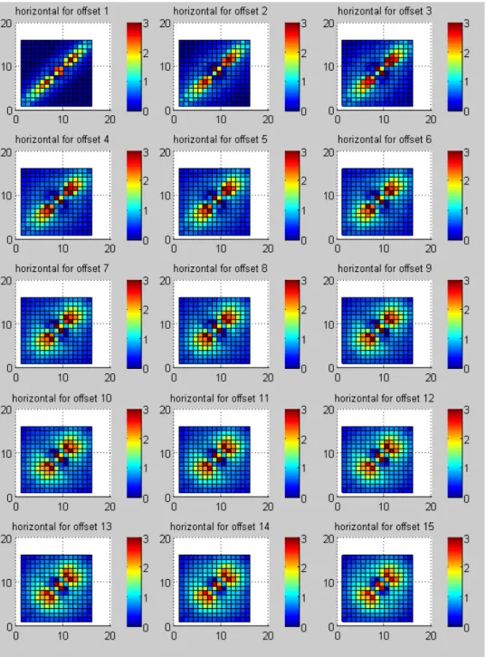
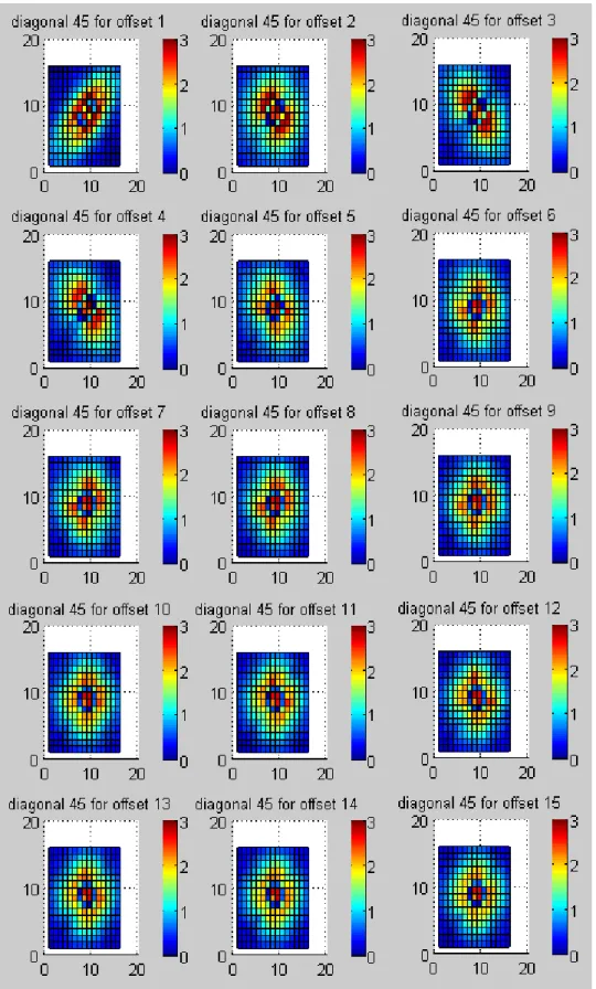
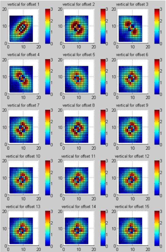
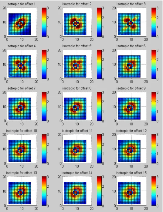
The following figures display the Mahalanobis distance between GLCMs for class 1 and 2 given the window size 51x51 for horizontal (3.4), diagonal 45°(3.5), vertical (3.6) and isotropic (3.7) directions depending on the dis-tance.

Distance matrices for size 31x31 look pretty similar and were not included in this report. We built the plots for norm of Mahalanobis distance matri-ces depending on the offset and direction, to find the optimal GLCM pa-rameters - they correspond to the point where norm reaches the maximum value. Figure 3.8 contains the norms plot for window size 31x31, and figure 3.9 contains the same for window 51x51.

As we see from the plots 3.8 and 3.9, the maximum norm is observed for the following GLCM parameters: window size 51x51, isotropic direc-tion, offset 2. These parameters help discriminate between GLCMs for two classes in the best way. The best discrimination is given by the vertical

and isotropic directions, and this is an expected result, because the first class has mostly sub-horizontal textures and significantly changes in verti-cal direction, while salt has low variance and almost does not change the amplitude regardless of direction. For the same reason, the distance for the

horizontal direction grows slowly with the offset: brightness varies very little in horizontal direction neither for salt, nor for sediments, and starts growing only on big offsets when steep-dipping reflectors become impor-tant. Norms for both diagonal directions, as expected, act as an average between vertical and horizontal.

Figure 3.10 displays the distance matrix between the class centers for isotropic direction and offset 2, the optimal direction and offset in terms of discrimination between two classes as shown above.

In the next chapter we will use the optimal GLCM parameters received in this chapter to test two hypotheses. First, whether the distance matrix can be used as a new GLCM feature and what is the classification performance compared to the standard GLCM features described in Chapter 2. Second, whether weighting the GLCM for each pixel with distance matrix improves the classification accuracy for the standard GLCM features.

Figure 3.4: Distance matrices plots in horizontal direction by distance, window 51x51.

Figure 3.5: Distance matrices plots in diagonal 45°direction by distance, window 51x51.

Figure 3.6: Distance matrices plots in vertical direction by distance, window 51x51.

Figure 3.7: Distance matrices plots in isotropic direction by distance, window 51x51.

Figure 3.8: Plot of Mahalanobis distance between two classes depending on direction and offset for window size 31x31.

Figure 3.9: Plot of Mahalanobis distance between two classes depending on direction and offset for window size 51x51.

(a) (b)

Figure 3.10: Distance matrix for isotropic direction and offset 2, window size 51, seen from two viewpoints.

Chapter 4

Evaluation

In this chapter we investigate whether a distance matrix between class cen-ters can be used as a new GLCM feature, and whether weighting with the distance matrix improves the performance of such standard GLCM fea-tures as Contrast, Homogeneity, Energy and Correlation.

4.1

Training a Gaussian classifier

As mentioned in the previous chapter, we were provided with one inline image and a training mask with two mapped classes. For each pixel of the training image we have computed standard GLCM features provided by Matlab, our own GLCM feature based on Mahalanobis distance matrix, four weighted GLCM features (same features from Matlab computed from GLCM multiplied with distance matrix), and variance. Variance was taken for comparison, as a first-order statistical feature. Totally, we had 10 fea-tures computed for each pixel, listing A.1 is provided in appendix.

We trained the Gaussian classifier both on one feature at a time, and on combinations of two and three features, and compared the results on a training set. The Matlab code for training a classifier is provided in list-ing A.2.

4.2

Classification results

4.2.1 Classification results on the training data set

We were provided the inline image and mask with two classes for training. We trained multiple Gaussian classifiers with dimensions from 1 to 3 on a subset of mask elements (ten percent from each class), selecting various combinations of above mentioned ten features. Then, we tested the per-formance of the classifiers on a training set to compare the original GLCM features with weighted and with our own GLCM feature based on Maha-lanobis distance between two classes. The results for Gaussian classifier

trained on one feature at a time are shown in table 4.1. TN rate stands for true negatives rate (percentage of correctly classified sub-horizontal re-flectors), FP rate - false positives rate (sub-horizontal reflectors classified as salt), TP - true positives (correctly classified salt), and FN - false neg-atives (salt classified as sub-horizontal reflectors). Sum of TN and FP is equal 100%, same for sum of TP and FN. The results for 2 and 3 features are shown in table 4.2.

Feature TN rate FP rate TP rate FN rate Variance 83,77 16,22 95,67 4,32 Contrast 91,52 8,47 97,17 2,82 Energy 94,73 5,26 82,81 17,18 Correlation 65,67 34,32 81,90 18,09 Homogeneity 92,78 7,21 90,92 9,07 Distance (own feature) 90,92 9,07 93,13 6,86 Weighted Contrast 93,52 6,47 96,05 3,94 Weighted Energy 95,35 4,64 77,61 22,38 Weighted Correlation 59,37 40,62 78,69 21,30 Weighted Homogeneity 94,68 5,31 91,01 8,98 Table 4.1: Comparison of classification results for classifier trained on one feature

Feature TN rate FP rate TP rate FN rate Contrast and Energy 94,17 5,82 91,80 8,19 Energy and Homogeneity 93,48 6,51 85,92 14,07 Contrast and Correlation 95,15 4,84 99,20 0,79 Energy and Distance (own) 94,14 5,85 86,64 13,35 Contrast and Distance 92,89 7,10 97,51 2,48 Energy and Variance 89,44 10,55 92,10 7,89 Energy, Distance and Variance 99,96 0,03 12,28 87,72 Contrast, Energy and Own 100,00 0,00 20,59 79,40 Contrast, Distance and Weighted Energy 98,42 1,57 82,80 17,19 Table 4.2: Comparison of classification results for classifier trained on two

features

4.2.2 Classification results on training and test images

However, testing the classifier just on a mask dataset is not completely cor-rect. In addition, we have to check how good the classifier performs on the entire training image, as well as on other inline images. The figure 4.1 shows an example inline image with manually delimited salt borders. It can be used as a reference image to compare classification results. Original inline input image used for training and evaluation is presented in figure

Figure 4.1: Example of inline section with manually interpreted salt borders.

4.2.

The following figures show the classification of the original inline image by variance (4.3), Contrast (4.4), Energy (4.5), Correlation (4.6), Homogeneity (4.7) and own GLCM feature - Distance - based on distance matrix (4.8). The visually best result is shown by a feature combination of Contrast, Dis-tance and Weighted Energy, both on original training image (4.13) and on test inline image (4.14).

Figure 4.2: Original inline image used for training and evaluation (normalized).

(a) (b)

Figure 4.3: Original inline image classification by variance.

(a) (b)

Figure 4.4: Original inline image classification by Contrast.

(a) (b)

Figure 4.5: Original inline image classification by Energy.

(a) (b)

(a) (b)

Figure 4.7: Original inline image classification by Homogeneity.

(a) (b)

Figure 4.8: Original inline image classification by Distance.

(a) (b)

Figure 4.9: Original inline image classification by Energy and Distance.

(a) (b)

Figure 4.10: Original inline image classification by Energy and Variance.

(a) (b)

Figure 4.11: Original inline image classification by Energy, Distance and Variance. Overtraining due to singularity in features.

(a) (b)

Figure 4.12: Original inline image classification by Contrast, Energy and Distance. Correlation is present in features.

(a) (b)

Figure 4.13: Original inline image classification by Contrast, Distance and Weighted Energy. Visually the best result.

(a) (b)

Figure 4.14: Test inline image (inlinekorr700) classification by Contrast, Distance and Weighted Energy.

Chapter 5

Summary and Conclusion

In this chapter we sum up the main results of this thesis. The results are primarily based on the problems stated in the Introduction chapter and solved in chapters 3 and 4.

5.1

Thesis results

5.1.1 Covered theoretical background

In this thesis we discussed how the marine seismic images are collected and processed, and what the motivation for salt segmentation in seismic images is. We have discussed, which textures that are present on seismic images and their properties. We covered several statistical and image pro-cessing methods, the most important of them were gray level co-occurrence matrices and their features, and the multivariate Gaussian classifier.

5.1.2 Achieved results

The two main tasks were to provide a method for finding the optimal GLCM parameters for a given image dataset with pre-mapped classes, and to try to make use of Mahalanobis distance matrix in terms of salt structure classification. The first task was covered and solved in the third chapter, giving us the result that the greatest distance between average GLCMs for two classes for inline images from North Sea dataset is observed in isotropic direction, with offset 2 and window size 51. The two last parameters are dependent on the scale, but the method remains the same.

The second result was that the Mahalanobis distance matrix derived on the previous step, can be used to discriminate between two classes in a same way as standard GLCM features. It also gives a classification improvement, strengthening the most discriminating GLCM elements. The combination of Contrast, own GLCM feature called Distance and Weighted Energy has shown visually best results among all classifiers.

5.2

Further work

Despite the fact the aims stated in the Introduction chapter were reached, there are several ways for further research and improvements. First, only inline cuts from a single 3D dataset were used for training and testing. The same approach can easily be tested also on 3D seismic images, and also images from other seismic datasets. We managed to avoid any fine-tuning with regard only to this dataset and kept the computations as general as possible, so the method is likely to work on marine seismic images from other regions.

Second, we analyzed only 2D seismic images. However, all the seismic data is initially stored in a 3D cube, so the spacial pixel dependencies can be used for better classification performance. For example, with the in-creasing computational power of modern processors and parallel libraries, using a GLCM in 3D might provide some better results.

Third, to compare the GLCM feature performance, only one- and two-dimensional Gaussian classifiers have been used. An adaptive feature se-lection approach can be used, when on each step we choose the best dis-criminating feature and add or remove depending on whether overall per-formance has increased or decreased.

Fourth, the Mahalanobis distance matrix can be used as a feature, however, it is computed based on the input inline image and mask. It will likely work for a close inline image from the same dataset, but still, it is very scale- and size-dependent. It would be a great generalization if one man-ages to extract the formula based on the computed distance matrix, that can be used in the same general way, as standard GLCM features. The Maha-lanobis distance image for isotropic direction and offset 2, shown on a fig. 3.10, gives large weight to the central four elements and to sub-diagonal elements positioned on 2-3 element distance from the center. At the same time, it suppresses the values placed on 1-pixel distance from the central four elements. This is due to the low variance observed in salt structures.

Fifth, as described in the Background chapter, there are many other meth-ods for texture analysis in seismic images, from a simple variance in local window, to Fourier transform and Gabor filters. Gray level co-occurrence matrices were the main research method in this thesis, but classification performance is proven to be better when used in combination with other texture description features.

Sixth, in this thesis we have focused on pixel-wise classification, without covering the methods of salt texture segmentation. There are also various approaches like connected-component analysis and morphological opera-tions that help to provide more exact salt region borders. In addition, seg-mentation can be done by segseg-mentation algorithm directly, without doing pixel-wise classification.

Appendix A

Listings of some of Matlab

scripts used in the thesis

Listing A.1: Computing GLCM features for classification

% Load i n l i n e i m a g e and mask

load( ’ i n l i n e _ 8 5 0 5 _ k o r r . mat ’ ) ; % P r e p a r e i n l i n e i m a g e downLimit = −100; upLimit = 1 0 0 ; i n l i n e I m g ( i n l i n e I m g < downLimit ) = downLimit ; i n l i n e I m g ( i n l i n e I m g > upLimit ) = upLimit ; i n l i n e I m g = normalize2D ( i n l i n e I m g ) ; % S e t GLCM p a r a m e t e r s g r a y L e v e l s = 1 6 ; halfWin = 2 5 ; d i s t = 2 ; % Load w e i g h t m a t r i x f o r i s o−2, window 51

load( ’ weight−i s o 2−win51−l e v 1 6 . mat ’ ) ;

% Compute GLCMs f o r a l l p i x e l s % o f c l a s s 1 i n i s o t r o p i c d i r e c t i o n glcms1 = getAllGlcms ( i n l i n e I m g , i n d i c e s 1 , . . . c l a s s 1 , halfWin , grayLevels , d i s t ) ; % C a l c u l a t e GLCM f e a t u r e s − s t a n d a r d (1−4) , % own ( 5 ) and w e i g h t e d s t a n d a r d (6−9) disp( ’ C a l c u l a t e d glcms1 ’ ) ; f o r i = 1 :length( glcms1 ) glcm = glcms1 ( i ) . glcm ; props = graycoprops ( glcm ) ; CL1 ( i , 1 ) = props . C o n t r a s t ; CL1 ( i , 2 ) = props . Energy ;

CL1 ( i , 3 ) = props . C o r r e l a t i o n ; CL1 ( i , 4 ) = props . Homogeneity ; % own GLCM f e a t u r e CL1 ( i , 5 ) = sum(sum_{( d i s t M a t r i x . * s i n g l e ( glcm ) ) ) ;} newProps = . . . graycoprops ( u i n t 8 ( d i s t M a t r i x . * s i n g l e ( glcm ) ) ) ; CL1 ( i , 6 ) = newProps . C o n t r a s t ; CL1 ( i , 7 ) = newProps . Energy ; CL1 ( i , 8 ) = newProps . C o r r e l a t i o n ; CL1 ( i , 9 ) = newProps . Homogeneity ; end

Listing A.2: Gaussian classification

c l e a r a l l; % l o a d a l l f e a t u r e maps ( p i x e l −> f e a t u r e v a l u e ) load( ’ t r a i n i n g _ d a t a _ w i n 5 1 _ l e v 1 6 _ i s o 2 ’ ) ; % PICK ONE f e a t u r e t o t r a i n a c l a s s i f i e r f e a t u r e = 1 ; featureName = ’ C o n t r a s t ’ ; % f e a t u r e = 2 ; f e a t u r e N a m e = ’ Energy ’ ; % f e a t u r e = 3 ; f e a t u r e N a m e = ’ C o r r e l a t i o n ’ ; % f e a t u r e = 4 ; f e a t u r e N a m e = ’ Homogeneity ’ ; %f e a t u r e = 5 ; f e a t u r e N a m e = ’ diffGLCM ( own ) ’ ; % f e a t u r e = 6 ; f e a t u r e N a m e = ’ W e i g h t e d C o n t r a s t ’ ; % f e a t u r e = 7 ; f e a t u r e N a m e = ’ W e i g h t e d Energy ’ ; % f e a t u r e = 8 ; f e a t u r e N a m e = ’ W e i g h t e d C o r r e l a t i o n ’ ; % f e a t u r e = 9 ; f e a t u r e N a m e = ’ W e i g h t e d Homogeneity ’ ; % f e a t u r e = 1 0 ; f e a t u r e N a m e = ’ V a r i a n c e ’ ; % T r a i n i n g f o r c l a s s 1 mean1 = mean( CL1 ( : , f e a t u r e ) ) ; cov1 = cov( CL1 ( : , f e a t u r e ) ) ; % assume e q u a l c l a s s p r o b a b i l i t y prob1 = 0 . 5 ; % T r a i n i n g f o r c l a s s 2 mean2 = mean( CL2 ( : , f e a t u r e ) ) ; cov2 = cov( CL2 ( : , f e a t u r e ) ) ; prob2 = 0 . 5 ; c l a s s i f i c a t i o n R e s u l t = z e r o s(s i z e( i n l i n e I m g ) ) ; f o r i = 1 : elements1 x = CL1 ( i , f e a t u r e ) ; % C a l c u l a t e G a u s s i a n f o r c l a s s 1 and 2

r e s 1 = c a l c G a u s s i a n ( x , mean1 , cov1 , prob1 ) ; r e s 2 = c a l c G a u s s i a n ( x , mean2 , cov2 , prob2 ) ;

r e s u l t 1 ( i ) = ( r e s 1 >= r e s 2 ) ; x = c l a s s 1 ( i n d i c e s 1 ( i ) ) . X ; y = c l a s s 1 ( i n d i c e s 1 ( i ) ) . Y ; i f r e s 1 >= r e s 2 c l a s s i f i c a t i o n R e s u l t ( x , y ) = 1 0 0 ; % c l a s s 1 e l s e c l a s s i f i c a t i o n R e s u l t ( x , y ) = 2 5 5 ; % c l a s s 2 end end % Do t h e same f o r c l a s s 2 . . . % C a l c u l a t e t r u e n e g a t i v e , f a l s e p o s i t i v e , e t c . TN = length(find( r e s u l t 1 = = 1 ) ) ; TN_rate = TN / elements1 ; FP = length(find( r e s u l t 1 = = 0 ) ) ; F P _ r a t e = FP / elements1 ; TP = length(find( r e s u l t 2 = = 1 ) ) ; TP_rate = TP / elements2 ; FN = length(find( r e s u l t 2 = = 0 ) ) ; FN_rate = FN / elements2 ; % C a l c u l a t e o v e r a l l c l a s s i f i c a t i o n r a t e o v e r a l l _ r a t e = (TN + TP ) / ( elements1 + elements2 ) ;

Bibliography

[1] F. Albregtsen. Statistical texture measures computed from gray level co-occurrence matrices, 2008.

[2] A. Berthelot, A. Solberg, and L.-J. Gelius. Texture attributes for detection of salt. Journal of Applied Geophysics, (88):52–69, 2013.

[3] A. Berthelot, A. Solberg, E. Morisbak, and L.-J. Gelius. Salt diapirs without well defined boundaries — a feasibility study of semi-automatic detection. Geophysical Prospecting, 59:682–696, 2011.

[4] A. Bhattacharyya. On a measure of divergence between two statistical populations defined by their probability distributions. Bulletin of the Calcutta Mathematics Society, 35:99–109, 1943.

[5] D. Clausi and Y. Zhao. Grey level co-occurrence integrated algorithm (glcia): a superior computational method to rapidly determine co-occurrence probability texture features. Computers and Geosciences, (29):837–850, 2003.

[6] R. Duda, P. Hart, and D. Stork. Pattern Classification, Second Edition.

Wiley Interscience, 2001.

[7] J. Gotlieb and H. Kreyszig. Texture descriptors based on co-occurrence matrices. Computer Vision, Graphics, and Image Processing, 51:70–86, 1990.

[8] A. Halpert and R. Clapp. Salt body segmentation with dip and frequency attributes. InSEP-Report 136, 2008.

[9] D. Hand.Discrimination and Classification. John Wiley and Sons, 1981. [10] R. Haralick. Statistical and structural approaches to texture.

Proceed-ings of the IEEE, 67(5):786–804, 1979.

[11] R. Haralick, K. Shanmugam, and I. Dinstein. Textural features for image classification. IEEE Transactions on Systems, Man, and Cybernetics, SMC-3:610–621, 1973.

[12] J. Lomask, R. Clapp, and B. Biondi. Application of image segmenta-tion to tracking 3d salt boundaries. Geophysics, 72(4):47–56, 2007. [13] P. C. Mahalanobis. On the generalised distance in statistics.Proceedings

[14] J. Schlaf, T. Randen, and L. Sønneland. Introduction to seismic texture.

Mathematical Methods and Modelling in Hydrocarbon Exploration and Production, 59:3–21, 2005.

[15] A. Solberg. Multivariate classification (inf4300), 2013.

[16] A. Solberg, A. Berthelot, and L. Gelius. Gabor filters for segmentation of salt structures. InExtended Abstract, 73rd EAGE Conference, 2011. [17] A. Solberg and L. Gelius. New texture attributes from local 2d fourier

spectra.SEG Technical Program Expanded Abstracts, 30:1165–1169, 2011. [18] A. Tiapkina, Y. Tyapkin, and A. Okrepkyj. Advanced methods for seismic imaging when mapping hydrocarbon traps associated with salt domes.Geophysical journal, 3:86–104, 2014.

[19] J.-M. Wu and Y.-C. Chen. Statistical feature matrix for texture analysis.

Computer Vision, Graphics, and Image Processing; Graphical Models and Image Processing, 54:407–419, 1992.