Improving Electrical Impedance Tomography of brain function with a novel servo-controlled electrode helmet

of brain function with a novel

servo-controlled electrode helmet

James Peter Avery

A dissertation submitted in partial fulfilment of the requirements for the degree of

Doctor of Philosophy of

University College London.

Department of Medical Physics & Biomedical Engineering University College London

I, James Peter Avery, confirm that the work presented in this thesis is my own. Where infor-mation has been derived from other sources, I confirm that this has been indicated in the thesis.

Conducting PhD research over the past four years has allowed me to make a living through investigating problems I find interesting, for which I feel extremely privileged. I am profoundly grateful to the people who supported me during this work, without whom this thesis would not have been possible. First I would like to thank my supervisors Prof. David Holder and Dr. Ben Hanson for offering me the opportunity to work on such a stimulating project, this work is a testament to their patience, encouragement, and experience.

Good research is collaborative and I am indebted to all of my friends in the UCL EIT group for their assistance, without their contributions none of the work would have been possible. I am especially thankful to Dr. Kirill Aristovich, whose advice and support in nearly every aspect in the project was invaluable, particularly in helping with the Sisyphean task of 3D printer maintenance. I would like to thank Dr. Thomas Dowrick who developed the UCL EIT system used in this project, and Bishal Karki who dedicated many hours to helping me with the KHU EIT system. Throughout the project I utilised software written by Dr. Gustavo Sato dos Santos, Dr. Aristovich and Markus Jehl for calculation of the forward solution and image reconstruction. The work on the head tank with skull is particularly indebted to Tugba Doru who first demonstrated the methodology. Dr. Brett Packham was a great support to me on innumerable tasks, but the advice and perspective on my research were especially appreciated. I must also acknowledge all past and present members of the UCL EIT group, whose work laid the foundations for my own.

I would also like to thank Dr. Aristovich, Nir Goren and Dr. Santos for helping me maintain my sanity and sharing horror stories during the early days of becoming a father. Finally I am grateful to my partner Catherine Evans, and my parents and sister, for their support and unwavering confidence in my abilities. I would like to dedicate this work to my son, Isaac, whose arrival brought things into perspective, albeit a hazy sleep deprived one.

Electrical Impedance Tomography (EIT) is a medical imaging technique which reconstructs the internal conductivity of an object from boundary measurements. EIT has the potential to provide a novel means of imaging in acute stroke, epilepsy or traumatic brain injury. Previous studies, whilst demonstrating the potential of the technique, have not been successful clinically. The work in this thesis aims to address fundamental limitations including measurement drift in electronic hardware, lack of an anatomically realistic tank phantom for rigorous testing, poor electrode-skin contact and mis-location of scalp electrodes. Chapter 1 provides an introduction of the principles of bioimpedance and EIT, as well as a review of previous clinical studies. Chapter 2 details the development of a novel anatomically realistic head phantom, simulating the human adult head with scalp electrodes, using a 3D printer and cylindrical holes to provide simulated conductivity. This replicated the varying spatial conductivity of the skull within 5 % of the true value. Two multifrequency EIT systems with parallel voltage recording were optimised for recording in the adult head with scalp electrodes, in chapter 3. Measurement drift was reduced by better case design and temperature control and data quality was improved with an updated interface to the current source and signal processing. The UCL ScouseTom system, performed best, with lower noise in all resistor and tank measurements, but the differences were masked during scalp recordings. Further, both systems produced similar results in the realistic adult head tank from chapter 2. Recent advances in EIT imaging coupled with the developments in chapters 2 and 3 provided opportunity to reassess the feasibility of monitoring epilepsy with EIT. Biologically representative perturbations was localised to within 8 mm in the head tank, with less than half the image error of previous studies. However, the key limitations of application time and measurement drift with scalp electrodes had yet to be addressed. Therefore the focus of the work in chapter 5 and chapter 6 was the design and testing of a novel self-adjusting electrode helmet. Skin-electrode impedance was continuously optimised by constant pressure, rotation and feedback control, and position sensors returned the co-ordinates of electrode tips. Finally, experiments with this helmet were undertaken to assess the feasibility of future clinical recordings.

1 Introduction and review 1

1.1 Brain Pathologies . . . 2

1.1.1 Acute stroke . . . 2

1.1.2 Traumatic Brain Injury . . . 2

1.1.3 Epilepsy . . . 3

1.2 Electrical Impedance Tomography . . . 5

1.2.1 Bioimpedance . . . 5

1.2.2 Instrumentation . . . 6

1.2.3 Protocols and data acquisition . . . 8

1.2.4 Imaging principle . . . 10

1.2.5 Imaging modalities . . . 11

1.2.6 Modelling errors in EIT . . . 13

1.3 EIT of brain pathologies . . . 16

1.3.1 Bioimpedance of stroke . . . 16

1.3.2 Bioimpedance of intracranial bleeding . . . 17

1.3.3 Bioimpedance of epilepsy . . . 18

1.3.4 Data collection and electrode localisation . . . 19

1.3.5 Summary of previous studies . . . 20

1.4 Biomedical electrodes . . . 20

1.4.1 Electrode - tissue interface and contact impedance . . . 20

1.4.2 Measurement Drift . . . 24

1.4.3 Electrodes and electrode placement . . . 26

1.5 Rationale . . . 30

1.5.1 Intended application . . . 30

1.5.2 Helmet specification . . . 31

1.6 Purpose . . . 32

1.7 Statement of originality . . . 34

2 Novel head tanks for EIT 37 2.1 Introduction . . . 37

2.1.1 Skull conductivity . . . 38

2.1.2 Head phantoms in EIT . . . 41

2.1.3 Modelling conductivity . . . 44

2.1.4 Reproducibility of tanks . . . 45

2.1.5 Purpose . . . 46

2.2.2 Electrode Positioning . . . 48

2.2.3 Tank design . . . 49

2.2.4 Anatomically realistic skull design . . . 50

2.2.5 Construction . . . 54 2.2.6 Geometry testing . . . 58 2.2.7 Comparison to simulation . . . 59 2.3 Results . . . 60 2.3.1 Geometry analysis . . . 60 2.3.2 Comparison to simulation . . . 60 2.4 Discussion . . . 65 2.4.1 Geometry of phantoms . . . 65 2.4.2 Comparison to simulation . . . 66 2.4.3 Assessment of tanks . . . 68

2.4.4 Reproducibility and limitations of method . . . 69

2.4.5 Technical considerations . . . 70

2.4.6 Recommendations for Further Work . . . 70

3 Comparison of two EIT systems 71 3.1 Introduction . . . 71 3.1.1 EIT systems . . . 72 3.1.2 Purpose . . . 76 3.1.3 Experimental Design . . . 77 3.2 Methods . . . 78 3.2.1 KHU Modifications . . . 78 3.2.2 ScouseTom Modifications . . . 86

3.2.3 Resistor Phantom Measurements . . . 91

3.2.4 Tank Measurements . . . 95

3.2.5 Scalp Recordings . . . 98

3.2.6 Test object complexity . . . 99

3.3 Results . . . 99

3.3.1 Resistor Phantom Measurements . . . 99

3.3.2 Head Tank . . . 104

3.3.3 Scalp Recordings . . . 111

3.3.4 Test Object Complexity . . . 112

3.4 Discussion . . . 115

3.4.1 System Comparison . . . 115

3.4.2 Technical considerations . . . 117

3.4.3 Implications for future experiments . . . 118

3.4.4 Recommendations for future work . . . 119

4 Feasibility of imaging epileptic seizures with EIT 121 4.1 Introduction . . . 121

4.1.1 Previous tank experiments . . . 121

4.1.2 Neonatal Tank Studies . . . 123

4.2.1 Tank Study . . . 125

4.2.2 Simulation Study . . . 128

4.3 Results . . . 129

4.3.1 Adult Head Tank . . . 129

4.3.2 Neonatal Head Tank . . . 132

4.3.3 Localisation Accuracy . . . 137 4.3.4 Signal Size . . . 140 4.4 Discussion . . . 142 4.4.1 Summary of results . . . 142 4.4.2 Tank study . . . 143 4.4.3 Simulation study . . . 143

4.4.4 Assessment of regularisation algorithms . . . 144

4.4.5 Study limitations . . . 145

4.4.6 Recommendations for future work . . . 146

5 Characterisation of abrasion 149 5.1 Introduction . . . 149

5.1.1 Purpose . . . 150

5.1.2 Experimental Design . . . 151

5.2 Methods . . . 152

5.2.1 Test object: skin analogue . . . 152

5.2.2 Overview of prototype and test rig . . . 154

5.2.3 Force control . . . 154 5.2.4 Rotary Actuation . . . 160 5.2.5 Impedance Measurement . . . 163 5.2.6 Electrode . . . 165 5.2.7 Methods validation . . . 167 5.2.8 Test protocol . . . 173 5.3 Results . . . 176

5.3.1 Characterisation of manual abrasion . . . 176

5.3.2 Contact impedance as a function of applied force . . . 177

5.3.3 Impedance during abrasion over a range of applied forces . . . 177

5.3.4 Impedance during abrasion for minimum and maximum applied torque 180 5.3.5 Proof of principle on human skin . . . 182

5.4 Discussion . . . 184

5.4.1 Summary of results . . . 184

5.4.2 Prototype performance . . . 186

5.4.3 Technical considerations . . . 187

5.4.4 Future work: implications for future designs . . . 189

6.1.1 Background . . . 191 6.1.2 Purpose . . . 194 6.1.3 Experimental Design . . . 194 6.2 Methods . . . 194 6.2.1 Electrode Unit . . . 194 6.2.2 Controller . . . 199 6.2.3 32 Channel Helmet . . . 205 6.2.4 Experimental Protocol . . . 208 6.3 Results . . . 209 6.3.1 Single Unit . . . 209

6.3.2 Four channel system . . . 210

6.3.3 32 Channel Helmet . . . 210

6.4 Discussion . . . 212

6.4.1 Summary of results . . . 212

6.4.2 Assessment of helmet design . . . 213

6.4.3 Technical Considerations . . . 214

7 Discussion and future work 217 7.1 Summary of studies . . . 217

7.2 Head tanks . . . 217

7.3 EIT systems . . . 218

7.4 Time difference imaging in the head . . . 218

7.5 Electrode helmet . . . 218

7.6 Future work . . . 219

1.1 Equivalent circuit of a cell(a), extracellular resistanceR_ein parallel with the intracellular resistanceRi and the capacitance of the cell membraneCm,(b) Cole-Cole plot of this circuit . . . 6 1.2 Equivalent circuit of measurement in EIT adapted from Boone and Holder

[41]. I s: current source, Cout: output capacitance, Rout: output resistance,

C_ed (C_er): electrode capacitance on driving (receiver) electrode, R_ed (R_er): electrode resistance on driving (receiver) electrode, R1-R4: load resistance under the measurement,Ri: input resistance,Ci: input capacitance, andVcm: common-mode voltage . . . 7 1.3 (a)Improved Howland Circuit iHCP from Franco[47],(b)equivalent model

of current source . . . 7 1.4 Two EIT systems used in the UCL group,(a)the serial UCL Mk2.5 designed by

McEwan, Romsauerova, Yerworth,et al.[48]and(b)the fully parallel KHU Mk 2 by Oh, Wi, Kim,et al.[49] . . . 8 1.5 EIT electrode positions,(a)EEG 31 protocol, 27 electrodes placed according to

the extended EEG 10-20 psotions from Tidswell, Gibson, Bayford,et al.[53], (b)Spiral16, a subset of 16 electrodes chosen by Fabrizi, McEwan, Oh,et al.[54] 9 1.6 Finite element models in EIT, fig. 1.6a mesh from CT and MRI segmentation

of the head by Jehl, Dedner, Betcke,et al.[63], fig. 1.6b rat brain mesh by Aristovich, Santos, Packham,et al.[61] . . . 13 1.7 Existing tanks used in experiments in the UCL group,(a)a 2D cylindrical tank

and(b)a head shaped tank created by Tidswell, Gibson, Bayford,et al.[74] . 14 1.8 Comparison of simulated and measured voltages in cylindrical tank . . . 14 1.9 Artefacts due to modelling errors during experiments by Malone, Sato Dos

Santos, Holder,et al.[71]in a 2D cylindrical tank . . . 15 1.10 Comparison of simulated and measured voltages in UCL head tank[74] . . . . 16 1.11 Change in conductivity over frequency of normal brain tissue, ischaemic brain

tissue and blood, adapted from[82] . . . 17 1.12 Example of data collection for stroke EIT, photogrammetry markers are visible

above elastic cap . . . 19 1.13 Simple equivalent circuit model of electrode-gel-skin interface from[95]. . . . 21 1.14 Equivalent electrical circuit of the epidermis from[102] . . . 22 1.15 Frequency characteristics of skin impedance from from[102]represented as

values for the equivalent circuit in figure 1.14. Number of tape strippings given by numbers in parenthesis, Roman numerals denote corresponding data inRp andC_p . . . 22

1.17 Simulated reconstruction of Extradural Haematoma,pertis ideal reconstruc-tion, No N is the reconstruction without any noise, the remaining columns

correspond to the images with realistic measurement drift added . . . 25

1.18 Example of traditional cup and paste EEG electrodes . . . 27

1.19 Self abrading electrode from[113] . . . 27

1.20 Quinton Quik-prep system for ECG electrodes[114]. . . 28

1.21 Principle of dry microsprike electrode . . . 29

1.22 Example EEG headnets. Clockwise from top left: Easycap, EEG electrodes, geodesic headnet and Physiometrix headcap from[78] . . . 29

2.1 various skull conductivities . . . 38

2.2 Skull samples demonstrating tri-layered structure, with two outer "compact" bone layers and a inner spongey layer of diploe, from Tang, You, Cheng,et al. [128]. . . 39

2.3 Scatter plots demonstrating the correlation of skull resistivity with(a)thickness r=−0.596 and(b)percentage of diploer=−0.917 from Tang, You, Cheng, et al.[128] . . . 39

2.4 3D head phantoms for EIT,(a)spherical tank from Liston, Bayford, and Holder [127], (b)four shell agar tank from Sperandio, Guermandi, and Guerrieri [141],(c)EEG phantom from Collier, Kynor, Bieszczad,et al.[143]and(d) anatomically realistic phantom from Li, Tang, Dai,et al.[144] . . . 42

2.5 Neonatal head phantoms. (a)spherical tank by Tang, Oh, and Sadleir[140], (b)smoothed head shaped tank by Tang and Sadleir[36] . . . 44

2.6 Simulation of current flow through surface mimicking skull resistivity, from Doru, Avery, Aristovich,et al.[77]. . . 45

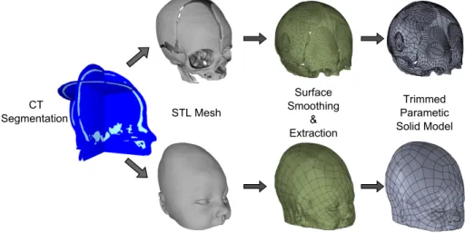
2.7 Workflow to create solid models from an MRI segmentation for the design of the adult tank . . . 48

2.8 Workflow to create solid models from a CT segmentation for the design of the neonatal tank . . . 48

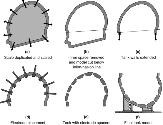
2.9 Design of tank models. (a)the scalp model is duplicated and scaled by 10%,(b) the inner scalp surface is removed and the shell split below in inion-nasion line, (c)the model is trimmed and the walls vertically extended 1cm,(d)models of the electrodes with clearance are positioned according to 2.2.2, (e), the clearance electrodes are removed from the tank volume,(f)Supports add and model is finalised . . . 50

2.10 Completed tank models for(a)adult head and(b)neonatal head . . . 51

2.11 Design of skull models. (a) the skull model is split below in inion-nasion line along the same plane as fig. 2.9,(b)the model is trimmed and the walls vertically extended 1cm to match the height of the tank walls,(c)a support base is added which is used to position the skull precisely in the tank, (d) cylinders are created centred around the points defined in 2.2.4 normal to the surface,(e), the cylinders are removed from the tank volume giving the final skull model . . . 51

2.14 Comparison ofσvalues for target and adjusted adult skull . . . 53

2.15 Skull conductivities from the literature in comparison with target and adjusted adult skull conductivities . . . 54

2.16 Completed skull models for(a)adult head and(b)neonatal head . . . 55

2.17 The 3D printer used to create the tanks, The Makerbot Replicator 2 from Makerbot Ind. . . 56

2.18 Completed phantoms for(a)adult head and(b)neonatal head . . . 57

2.19 Mesh of adult tank produced by 3D scanning . . . 59

2.20 Deviation analysis of head shaped tank . . . 60

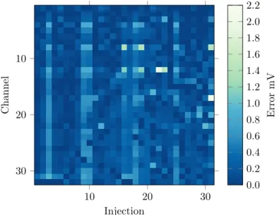
2.21 Comparison of voltages in adult head tank with optimal protocol . . . 61

2.22 Error Across injections in adult head tank with optimal protocolR=0.9985 . . 61

2.23 Comparison of simulated and measured voltages in neonatal head tankR=0.9992 62 2.24 Error in measured voltages across injections in neonatal head tank . . . 62

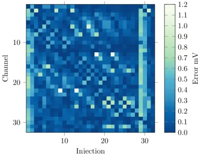
2.25 Comparison of voltages in adult head tank with skull with optimal protocol R=0.9985 . . . 63

2.26 Error Across injections in adult head tank and skull with optimal protocol . . . 63

2.27 Comparison of simulated and measured voltages in neonate head tank including skull phantomR=0.9972 . . . 64

2.28 Error in measured voltages across injections in neonate head tank including skull phantom . . . 64

2.29 Percentage errors in measured voltages . . . 65

3.1 Drift across an hour recording on the head with the UCH mk2.5, as percentage of baseline mean plus standard deviation . . . 72

3.2 Internal view of 16 channel KHU Mk 2 system, from which the 32 channel KHU Mk 2.5 system used in this study is descended, from Oh, Wi, Kim,et al.[49] . 72 3.3 Function blocks of the KHU Impedance Measurement Module (IMM), from Oh, Wi, Kim,et al.[49] . . . 73

3.4 Commercial components of the ScouseTo, EIT system,(a)BioSemi ActiveTwo EEG Amplifier and(b)Keithley 6221 Current Source . . . 74

3.5 Programming ST switch network. Source and sink channels set by pulses on +chn and -chn pins, injections pairs switched when sync pin set to high . . . . 76

3.6 Resistor set up for preliminary testing of the 32 channel KHU Mk 2.5 EIT system 79 3.7 Noise in voltages recorded on 1.1 kΩresistor during preliminary testing of the 32 channel KHU Mk 2.5 EIT system . . . 79

3.8 Comparison of the amplitude of the sine wave across 1.1 kΩresistors, top: as calculated from the rms of voltage collected with a NI USB DAQ, bottom: the output from the KHU system . . . 80

3.9 Updated regulator board for 32 Channel KHU Mk. 2.5,(a)circuit diagram . . 81

3.10 Improved power supply design for KHU 32 channel system . . . 81

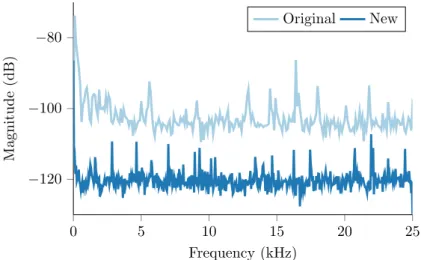
3.11 PSD of the voltage from KHU+5V regulator for original and new design,(a) with system idle(b)with system in scan mode . . . 82

3.12 PSD of the voltage from KHU 3.3 V regulator for original and new design with system in scan mode . . . 83

3.14 Comparison of signal to noise ratio of injected current for the KHU mk2.5 with increasing current level setting . . . 85 3.15 Switch Network Controller for ST EIT system: Switch network PCB and Arduino

Uno with shield in 3D printed housing . . . 87 3.16 Overview of ScouseTom EIT system. Current source and switch network

con-trolled via Serial communication and Matlab interface. Switching indicators sent to BioSemi Digital Input channels . . . 88 3.17 Ringing artefact in ScouseTom demodulation . . . 90 3.18 Effect of increasing truncation samples for 3rd and 5th order IIR filters and

increasingN . . . 90 3.19 Four terminal measurement set-up. Injecting electrodes connected to terminals

1 and 2, measurement electrodes connected to terminals 3 and 4 . . . 91 3.20 Circuit diagram of SwissTom Resistor Phantom[165] . . . 92 3.21 Example four terminal recording with both systems. KHU begins to overheat

after 220 repeats . . . 93 3.22 Section view of conductivities in hexahedral mesh of head tank. (a)baseline

conductivity of saline and skull,(b)“ideal” perturbation in posterior location 96 3.23 Three locations of perturbations used in tank study, based on positions from

Malone, Jehl, Arridge,et al.[59]. . . 96 3.24 Scalp electrode locations, based on the

spiral_16

McE-wan, Oh,et al.[58] . . . 99 3.25 Noise in four-terminal measurements across expected load range, comparison

of ST and KHU systems . . . 100 3.26 Variation across current of transimpedance V

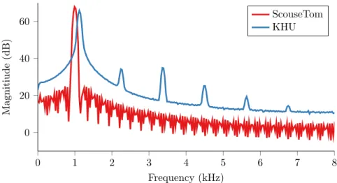
Arecorded on SwissTom resistor phantom with the ST and KHU EIT systems. Top: average transimpedance across all channels, bottom : standard deviation transimpedance across channels101 3.27 PSD of ScouseTom and KHU EIT systems with 1kHz and 1.125 kHz current

injection respectively . . . 101 3.28 Variations of the voltages measured on the SwissTom resistor phantom across

frequency with the ST and KHU EIT system . . . 102 3.29 Noise in hour long recording on resistor phantom . . . 103 3.30 Mean and standard deviation of drift across channels over one hour recording

on SwissTom phantom with ST and KHU systems . . . 103 3.31 Inter channel variations in one hour long recording on four separate protocol

combinations, expressed as relative standard deviation. R_{l oad} = 4.48 for combination 1 and 2,R_{l oad} =15.8 for combinations 3 and 4 . . . 104 3.32 Comparison of baseline voltages measured in adult head tank with ST and KHU

systems to respective simulations . . . 105 3.33 Percentage errors of measurements from ST and KHU systems in comparison

to simulation . . . 105 3.34 Standard deviation of recordings in adult head phantom . . . 106

with KHU.(a)full range highlighting skull sensitivity with ST,(b)narrower range displaying differences inside skull and(c) expressed as a percentage change . . . 106 3.36 Simulated reconstructed perturbations for corresponding measurement

proto-col in comparison to ideal perturbation . . . 107 3.37 Section views of image of simulated reconstruction withposteriorperturbation

for ST and KHU measurement protocols . . . 108 3.38 Section views of image of simulated reconstruction withcentralperturbation

for ST and KHU measurement protocols . . . 108 3.39 Section views of image of simulated reconstruction withlateralperturbation

for ST and KHU measurement protocols . . . 109 3.40 Image error metrics for simulated reconstructions compared to “ideal”

pertur-bations, for(a)ScouseTom Protocol and(b)KHU protocol . . . 110 3.41 Reconstructed perturbations in adult tank with both ST and KHU systems, in

comparison to ideal reconstructions . . . 110 3.42 Section views of image of experimental reconstructions withposterior

pertur-bation for ST and KHU measurement protocols . . . 111 3.43 Section views of image of experimental reconstruction withcentral

perturba-tion for ST and KHU measurement protocols . . . 112 3.44 Section views of image of experimental reconstruction withlateralperturbation

for ST and KHU measurement protocols . . . 113 3.45 Image error metrics for experiments compared to simulated perturbations for

(a)ScouseTom Protocol and(b)KHU protocol . . . 113 3.46 Standard deviation of recordings in adult head phantom . . . 114 3.47 Proportional noise as % of mean across all experiments, resistor phantom,

saline tank and scalp . . . 114 4.1 Lateral perturbation reconstructions in anatomically realistic head tanks. True

3D reconstructions,(a)30 % contrast Fabrizi, McEwan, Oh,et al.[58],(b)90 % contrast without skull Packham, Koo, Romsauerova,et al.[68]and(c)90 % contrast with skull. 2D reconstructions,(d)176 % contrast Li, Tang, Dai,et al. [144]and(e)2000 % contrast Dai, Li, Hu,et al.[16]. . . 122 4.2 Time difference image of 50 % contrast representing intraventricular

haemor-rhage in neonatal head tank without skull Tang and Sadleir[36] . . . 123 4.3 Perturbation locations used in tank study,(a)adult tank based on positions from

Malone, Jehl, Arridge,et al.[59]and(b)neonatal tank with two additional locations . . . 125 4.4 Perturbations in adult tank, reconstructed with both zeroth and first order

Tikhonov, in comparison to ideal reconstructions . . . 130 4.5 Section views of image of experimental reconstructions withposterior

pertur-bation with both zeroth and first order Tikhonov regularisation . . . 131 4.6 Section views of image of experimental reconstructions withcentral

4.8 Image quantification results in adult tank,(a)zeroth order and(b)first order Tikhonov regularisation . . . 133 4.9 Perturbations in neontal tank, reconstructed with both zeroth and first order

Tikhonov, in comparison to ideal reconstructions . . . 134 4.10 Section views of image of experimental reconstructions withanterior

pertur-bation with both zeroth and first order Tikhonov regularisation . . . 135 4.11 Section views of image of experimental reconstructions withposterior

pertur-bation with both zeroth and first order Tikhonov regularisation . . . 135 4.12 Section views of image of experimental reconstructions withlateral

perturba-tion with both zeroth and first order Tikhonov regularisaperturba-tion . . . 136 4.13 Section views of image of experimental reconstructions withcentral

perturba-tion with both zeroth and first order Tikhonov regularisaperturba-tion . . . 136 4.14 Section views of image of experimental reconstructions withcaudal

perturba-tion with both zeroth and first order Tikhonov regularisaperturba-tion . . . 137 4.15 Image quantification results in neonatal tank,(a)zeroth order and (b)first

order Tikhonov regularisation . . . 138 4.16 Localisation error (mean±std) of the simulated perturbations in(a)adult and

(b)neonatal head, with and without noise present, for both regularisations, expressed as norm of vector distance in mm, and as a percentage of mesh dimensions . . . 138 4.17 Spatial distribution of localisation error in mm in adult head for both zeroth

and first order Tikhonov regularisations, for simulated perturbations with and without realistic noise added . . . 139 4.18 Spatial distribution of localisation error in mm in neonatal head for both zeroth

and first order Tikhonov regularisations, for simulated perturbations with and without realistic noise added . . . 140 4.19 Median voltage changeµV for 10 % contrast perturbations across the adult

head,(a)sagittal section and(b)axial section . . . 140 4.20 Percentage of measurable voltages for a given minimum signal size inµV across

all perturbationspi jkin adult head, expressed as percentiles of the perturbation distribution . . . 141 4.21 Median voltage changeµV for 10 % contrast perturbations across the neonatal

head,(a)sagittal section and(b)axial section . . . 141 4.22 Percentage of measurable voltages for a given minimum signal size in µV

across all perturbationsp_{i jk}in neonatal head, expressed as percentiles of the perturbation distribution . . . 142 5.1 Diagram of experimental set up to determine expected load impedances . . . . 152 5.2 Impedance of orange peel sections before and after abrasion . . . 153 5.3 Overview of test rig, highlighting force control, rotary actuation and impedance

measurement components . . . 154 5.4 Schematic of force control components in prototype . . . 155 5.5 Free body diagram of force control system, with generic test object . . . 157

5.7 Limit cycling example . . . 159

5.8 Block Diagram of stepper feedback control, with dead band . . . 160

5.9 Limit cycling example . . . 160

5.10 Schematic of rotary actuation components . . . 161

5.11 Schematic of rotary actuation components, front view highlighting the trans-mission from DC motor to spindle . . . 161

5.12 Quadrature endcoder location, mounting hidden . . . 162

5.13 Phototransistor output for different codewheel track numbers. 10 and 20 track codewheels reliably decreased irradiance below threshold . . . 163

5.14 Block diagram of impedance measurement circuit . . . 164

5.15 Schematic of electrode design . . . 165

5.16 Comparison of electrode impedances of brass electrode and silver reference electrode . . . 166

5.17 Schematic of electrical connection of reference and actuated electrode, slip ring highlighted . . . 166

5.18 Power spectral density of noise from spindle and slip ring . . . 167

5.19 Error in resistance measurements with impedance measurement module (R_{I M M}) and Hewlett Packard 4284A Impedance Analyser (R_{H P}) . . . 168

5.20 Impedance of RC circuit, comparison of simulated and measured values . . . . 168

5.21 Resistance of RC circuit, comparison of simulated and measured values . . . 169

5.22 Reactance of RC circuit, comparison of simulated and measured values . . . 169

5.23 Averaged step response of orange peel . . . 170

5.24 Comparison of orange skin impedance before and after abrasion, and impedance of human skin with 0,9, and 15 strippings from[102]. Reduced frequency range in orange peel results due to limitations in measurement system . . . 171

5.25 Speed profile of electrode rotation . . . 172

5.26 Experimental setup to determine stall torqueT_{st al l} of motor from maximum forceFma x . . . 172

5.27 Stall torque (maximum torque available) profile of electrode rotation as a function of duty cycle . . . 173

5.28 Experimental setup to measure force applied during manual abrasion, and resultant impedance . . . 174

5.29 Experimental setup to measure impedance decrease during abrasion of the human . . . 175

5.30 Force profile during manual abrasion of test sample with abrasive paste and cotton bud . . . 176

5.31 Impedance spectra of orange skin test samples before and after manual abrasion176 5.32 Impedance as a function of force applied normal to surface . . . 177

5.33 Impedance decrease with respect to the number of rotations of the electrode, for a range of incident forces . . . 178

5.34 Impedance decrease with respect to abrasion time, for a range of incident forces178 5.35 Impedance decrease per sixth of a rotation, for a range of incident forces . . . 179

5.36 Impedance spectra of orange skin test samples before and after 20 seconds automated abrasion with 7.5 N applied force and 90 % duty cycle . . . 179

5.38 Comparison of impedance decrease for 5 N applied force with respect to number

of rotations for both minimum and maximum applied torque . . . 180

5.39 Comparison of impedance decrease for 5 N applied force with respect abrasion time for both minimum and maximum applied torque . . . 181

5.40 Minimum torque necessary to rotate electrode across range of applied forces . 181 5.41 Impedance decrease on human forearm with respect to the number of rotations of the electrode, with and without abrasive conductive paste. Note motion artefact at 1.5 rotations for without paste . . . 182

5.42 Impedance spectra measured on human forearm: before and after abrasion without paste (dashed); before and after abrasion with paste, and with the addition of paste only (solid) . . . 183

5.43 Comparisons of corrected impedance spectra after abrasion was complete for both wet and dry abrasion in comparison with the impedance after 9 and 15 strips from[102] . . . 183

6.1 Comparison of mean and standard deviation of head measurements in anthro-pometric surveys . . . 193

6.2 Miniaturised servo electrode unit. (a), overview of components,(b)concentric rotary actuation via servo motor with pain bearing and plain bearing, (c) feedback of electrode positionX_E through measurement of displacementX_P, (d) units placed in rigid helmet at known positions, (e) isometric view of complete unit . . . 195

6.3 Off the shelf components adapted for electrode unit,(a) Tower Pro MG90s Servo Motor,(b)BEI 9605 spring return linear position sensor . . . 196

6.4 Characterisation of spring return linear sensor. Stepper motor advances to compress spring onto load cell. Measurements of displacement obtained from laser displacement sensor . . . 197

6.5 Characterisation of spring potentiometer,(a)voltage across compression mean_±std, (b), force as function of distance mean±std . . . 198

6.6 Abrasive electrode patterns . . . 198

6.7 Wiring path to electrode . . . 199

6.8 Overview of helmet controller. Labview software controlling Arduino Due through wireless serial communication. Ardruino controls impedance measure-ment, servo rotation and electrode position measurements . . . 200

6.9 Control of 32 Servos using PCA9685 breakout boards . . . 201

6.10 Adafruit 815 servo controller in 3D printed casing . . . 201

6.11 Control of 32 Servos using PCA9685 breakout boards . . . 202

6.12 Impedance measurement circuit for helmet controller . . . 202

6.13 Standard deviation of impedance measurement for frequency of 20 and 100 Hz for increasing number of periods averaged . . . 203

6.14 Validation of impedance measurement circuit based on Arduino Due. (a), mean±std across expected measurement range compared to ideal,(b) percent-age error . . . 204

6.17 Design of electrode bearing helmet(a)the scalp model is scaled to match the nominal head dimensions section 6.1.1 and model trimmed below in inion-nasion line,(b)helmet frame constructed from 10 mm offset of nominal scalp surface,(c)electrode blocks are added to model and spacers then removed to create housings for each electrode unit aligned to the points in fig. 6.16,(d) electrode units added to complete model . . . 206 6.18 Comparison of mean and standard deviation of head measurements in

anthro-pometric surveys . . . 207 6.19 Final helmet model inclusive of electrode assemblies . . . 208 6.20 Abrasion with single miniature unit on orange skin test rig, for both pyramidal

electrode as in chapter 5, and smoothed electrode . . . 209 6.21 Abrasion with four channel system with application of abrasive Nuprep paste

and with EleFix EEG gel and Nuprep paste . . . 210 6.22 Long term recording with four channel system, with two actuated electrodes

and two conventional EEG electrodes, application of abrasive Nuprep paste and with EleFix EEG gel and Nuprep paste only . . . 211 6.23 Abrasion with 32 channel helmet on the scalp . . . 211 6.24 Minimum impedance with abrasion across range of compressions . . . 212

1.1 Summary of approximate head tissue conductivities below 1 MHz from Horesh [82] . . . 17 2.1 Conductivities of human skull from Tang, You, Cheng,et al.[128]measured at

1 kHz . . . 52 3.1 BioSemi ActiveTwo, EEG system specifications . . . 75 3.2 Keithley 6221 AC current source, system specifications . . . 75 3.3 Comparison of EIT systems used in this study . . . 76 3.4 SNR of injected current on the SwissTom resistor phantom as measured with

the BioSemi EEG system . . . 102 5.1 Orange Peel Impedances . . . 153 5.2 Load Cell Errors . . . 156 5.3 RMS error of force control system during abrasion . . . 177

Introduction and review

Electrical Impedance Tomography is a tomographic medical imaging technique which produces the internal electrical impedance of a subject from multiple impedance measurements using surface electrodes. Images are reconstructed by modelling electric fields within a Finite Element Model (FEM) of the subject and applying inverse algorithms. EIT has been proposed for a multitude of imaging techniques in the brain, including acute stroke and epilepsy. Electrodes must be placed onto the scalp before data acquisition, and the quality of the contact of the electrodes with the skin is an important factor in determining the signal to noise ratio of the EIT measurements. Conventional EEG cup electrodes, approximately 1 cm across, are commonly used in EIT studies on the head. The electrode site is prepared by an expert technician through removal of the top layer<1 mm of skin, through abrasion with an applicator and abrasive paste. To enable imaging of acute stroke in an ambulance or other acute setting, electrodes must be applied rapidly by unskilled personnel, the conventional methods are time consuming and labour intensive and are thus not practical. The purpose of this project was to design an electrode bearing helmet which automatically applies electrodes onto the scalp of the patient, achieving and maintaining a low contact impedance in a safe manner. Methodological developments in other areas of EIT were also undertaken as part of this work, in both the design of realistic head tanks, and modification of newly developed hardware for use in scalp recordings. Whilst the primary purpose of the helmet is to rapidly apply electrodes for imaging acute stroke, it also enabled control of the electrode contact throughout recordings, which is beneficial for a number of other EIT applications. Epilepsy monitoring with EIT was revaluated in light of the developments in imaging and hardware within the UCL group and this thesis, and the suitability of the helmet design assessed with

respect to this application alongside the primary purpose of imaging acute stroke.

1.1

Brain Pathologies

1.1.1

Acute stroke

Stroke is a major health problem, it is a leading cause of morbidity and disability in industri-alised nations[1]and the Department of Health estimates the annual direct cost to the NHS as £2.8 billion[2]. Stroke is caused by a lack of oxygen to part of the brain, and has two main causes: ischaemic, where bloody supply is interrupted due to a blood clot, and haemorrhagic due to a vascular rupture. Ischaemic strokes can be treated through the use of thrombolytic (or clot-dissolving) agents, but these are deleterious, or even potentially fatal, to patients suffering from haemorrhagic stroke. It is necessary therefore to be certain in the differentiation between the two types of stroke, which cannot be achieved without neuroimaging. The earlier the treatment through thrombolytics the better the outcome with the benefits limited to the first 3 to 6 hours after onset[3]. Therefore it is essential that neuroimaging and hence treatment is performed as soon as possible. However, studies have shown that transport to CT or MRI scanner and completion and reporting of the scan take at least an hour[4], and that the majority of stroke patients are arriving at emergency departments after 3 hours[5]. In the UK the NHS uses the time taken for “FAST positive” patients (i.e. those with a suspected stroke) to reach a hyperacute stroke centre as a quality indicatorDeptartmentofHealth2012 The most recent statistics for October 2011 show that 68.4 % of FAST positive patients arrived at the stroke centre within one hour of the call to the emergency services. The National Institute for Health and Clinical Excellence (NICE) clinical guidelines stipulates that brain imaging should be performed “immediately (within the hour)” for patients with a suspected stroke[6]. Therefore even if patients arrive at the unit within the one hour guideline, they are unlikely to have a CT or MRI taken within the treatment guidelines, which are also an hour. It is clear therefore that faster imaging of acute stroke is vital to prevent patients being denied essential treatment during this timeframe. Electrical Impedance Tomography has been proposed as a solution to enable early neuroimaging in ambulances or diagnostic centres without other scanning systems[7].

1.1.2

Traumatic Brain Injury

Traumatic brain injury (TBI) is defined as an insult or trauma to the brain from an external force[8]. TBI is a major health issue and is one of the leading causes of death and long term disability, with 1000 patients per 100,000 attend A & E with TBI, and 10 in 100,000 fatalities [8],[9]. TBI is the most common cause of death and disability in people aged 1-40 in the UK. The majority of fatal outcomes are in moderate or severe groups of the Glasgow Coma Scale (GCS)[10]which comprise of only 5 % of TBI patients[11]. Thus clinicians need to identify

a relatively small number of patients who will go onto develop serious acute intracranial problems. The majority of brain injuries could be detected in the first CT scan performed at emergency units with an established screening protocol to determine the urgency for each patient[11]. However, commonly there are secondary injuries with a delayed onset, such as Extradural Haematoma (EDH), subdural haematoma (SDH), and intracerebral Haemorrhage (ICH) which are not visible in the initial scans[11],[12]. In some of these cases, patients may have a normal initial CT scan, a high rating on the GCS indicating no alarming clinical signs, yet deteriorate and present significant findings in a subsequent CT scan. This delayed injury can be severe, even resulting in death. These delayed onsets are most likely to occur in the first two to three days after the primary injury, but have been known to occur weeks afterwards [12]. Monitoring these delayed onset brain injuries has been an application of EIT proposed early on the in the development of the technique[13]. Recently, studies by Manwaring, Moodie, Hartov,et al.[14]and Dai, Wang, Xu,et al.[15]have shown reproducible images of injected arterial blood in swine models with scalp electrodes. The most recent developments have shown in vivo images of injected irrigating fluid (5% dextrose in water) used in treatment of SDH[16]. Whilst this represents a step towards detection of intracranial bleeding, the dextrose mixture was injected in a known position, and has a conductivity contrast ten times greater than that expected through bleeding.

1.1.3

Epilepsy

Epilepsy is a neurological condition in which synchronised neuronal firing causes unpredictable recurring seizures. It is the most common neurological disorder, affecting approximately 50 million people globally[17], and accounts for 0.5% of the global burden of disease[18]. There are over 30 different types of epilepsy, and their categorisation and characterisation is still a cause for debate[19],[20]. Generally they can be categorised intofocal(orpartial) seizures, which are generated in and affect only a single area of the brain ranging from part of a lobe up to an entire hemisphere, andgeneralisedseizures which occur in both hemispheres of the brain [19]. Generalised seizures originate in networks which are distributed bilaterallyi.e. both hemispheres, and have onsets which can appear localised within in a single seizure, but are not consistently localised or lateralised between seizures. Focal seizures however, are constrained to networks within a single hemisphere and the ictal (seizure) onset is consistent between seizures, and are the most common type of seizure[21]. Generalised and focal seizures can occur both in superficial cortical structures of the brain, as well as deeper subcortical areas. Anti-epileptic drugs (AEDs) are the initial treatment for epilepsy patients, however they are not effective in 20-30 % of chronic cases[22], with approximately 60 % of patients with partial epilepsy entering remission with AED alone[23]. Patients who are not responding to AEDs, can potentially be treated through resective surgery, wherein the epileptogenic zone, the area of cortex generating the seizures, is removed or disconnected[24]. The outcomes of these

patients undergoing resective surgery is generally good, with 30 to 85 % remaining seizure free. However, surgery is only considered if the focus is clearly identified and subsequently deemed resectable if it is located in a accessible area of the brain and removal will not significantly impair brain function[25]. Therefore, there is a clear clinical need for accurate foci localisation in epilepsy patients. This is routinely localised with prolonged video-EEG monitoring, which provides EEG recordings and seizure semiology for generating a hypothesis as to the seizure onset zone. Often, for improved localisation, patients undergo intracranial EEG recordings (ECoG) with electrodes placed on the surface of the cortex where the epileptogenic focus is suspected to be, based on the scalp EEG[25],[26]. Although free of the attenuation and distortions of the skull and scalp, these ECoG recordings still have drawbacks relating to the fact that it is asummatedpotential recorded on the surface[27]. As such, activity may not have an EEG correlate if the source is located deep in the brain, or is orientated tangentially to the scalp, or cancelled out by an opposing source in the sulci. Depth electrodes can be placed to overcome these issues but as they damage brain tissue, are necessarily limited in their number and spacing[26]. Improved localisation of epileptic foci has been proposed as a potential application of EIT[28],[29], as an adjunct modality to conventional EEG or ECoG recordings[30].

Neonatal Epilepsy

Seizures in full term infants have been shown to occur in 0.5-3 per live 1000 births, and up to 13% of very low birth weight infants[31]. Swift intervention is important as continued seizures are linked with permanent cerebral damage and long-term neuro-developmental delay [32], [33]. The majority of neonatal seizures are acute and arise as symptoms of another brain injury, the most common of which are Hypoxic-ischaemic encephalopathy and intracranial haemorrhage[34]. A major challenge in the diagnosis of epilepsy in infants is electroclinical dissociation,i.e. there may be seizures visible in EEG recordings but not clinically and visa-versa. The exact incident of clinically silent seizures is as yet unknown[31]. The physiology of the neonatal brain presents additional challenges alongside the problems of attenuation and source orientation of conventional EEG. The incomplete myelinisation (insulation layer) and arborisation (branching) of axons and dendrites within the neonatal brain result in small, isolated, weakly propagated seizures, the activity of which may not spread to surface EEG electrodes[31]. This has been proposed as an explanation of the electroclinical dissociation, as the symptoms of the seizures are clinically observed, but the electrical activity does not propagate to the surface electrodes. A further explanation is that certain seizures may not be epileptic, but occur in the primitive brain stem or spinal motor cord, and thus are unlikely to have an EEG correlate[31]. Unlike in adult patients, resective surgery is uncommon in neonates with intractable epilepsy due to the associated risks[35]. Therefore the need for accurate localisation is less clearly defined as in adult patients. However, EIT has

been proposed as a method of both locating the activity in deeper structures[33], which could offer insight into the problem of electroclinical dissociation, as well as imaging intracranial haemorrhage, the major cause of seizures[36].

1.2

Electrical Impedance Tomography

Electrical Impedance Tomography (EIT) is an non-invasive imaging technique which exploits differences or changes in electrical properties of biological tissues to obtain structural or functional information. An array of electrodes are placed on the surface of the body, insensitive current is then injected and the resultant voltages are recorded. Images of the impedance distribution in two or three dimensions are reconstructed using an algorithm based on a formulation of Ohm’s law for current flow in a volume[37],[38]. The advantages of EIT, particularly in the case of imaging acute stroke, lie in the portability and low cost of the instrumentation and the high temporal resolution. The limitations however, are low spatial resolution and sensitivity to errors in modelling and instrumentation.

1.2.1

Bioimpedance

The impedanceZdescribes the electrical properties of a biological tissue when a current or voltage is applied. The extent to which the charge transport is opposed within the tissue is described by its resistanceR, and the capacitanceC describes the ability of the tissue to store charge. Current is conducted through ion diffusion within the conductive extra and intra cellular spaces within the cell, which can be modelled as resistancesReandRi, whereas the lipid cell membrane can be modelled as a capacitanceC_m[39]. The cell can thus be modelled as a simple parallel circuit, fig. 1.1a with frequency dependent impedance

Z(ω) = R_eR_i+ Re jωC_m R_e+R_i+ 1 jωCm . (1.1)

At low frequencies no current crosses the cell membrane Cm as it is predominantly fully charged

lim

ω→0Z(ω) =Re. (1.2)

As the frequency ωincreases, more current is diverted away from the extracellular re-sistance into the intracellular space, increasing the phase angle. At high frequencies the membrane capacitanceCm becomes negligible, soZ(ω)again becomes purely resistive

lim

ω→0∞Z(ω) = ReRi

Re+Ri

This frequency dependence is commonly displayed in acole-coleplot, fig. 1.1b, named after Cole and Cole[40]who extensively studied the frequency response of dielectrics.

Re Ri C_m (a)

ω

R

-

X

R

R

||R

ω

ω

Figure 1.1:Equivalent circuit of a cell(a), extracellular resistance Rein parallel with the intracellular

resistance Riand the capacitance of the cell membrane Cm,(b)Cole-Cole plot of this circuit

The value generally reconstructed in EIT is theconductivityσ, the inverse of theresistivity

ρ. It is the variations of the conductivity between brain tissues which is used in EIT to provide information regarding structure and function within the brain.

1.2.2

Instrumentation

The measurement problem in EIT can be modelled as an equivalent circuit, fig. 1.2. Most common EIT systems comprise of a constant current drive (Is) and a differential voltage measurement side. Impedance measurements are usually made using four electrodes in tetrapolar configuration (also known as Kelvin sensing), with alternating current injected between one pair of electrodes and the remaining pair used to measure voltage[41]. The precision of the instrumentation is a crucial factor in the accuracy of the reconstructed images. Due to the ill posed nature of the EIT inverse problem, small errors in voltage measurements can result in large changes in the reconstructed conductivity[42]. The majority of the errors in an EIT system arise from the impedanceCed Red which arises at the interface of the electrode with the boundary of the subject, known as thecontact impedance, the causes of which are discussed in detail in section 1.4.

The majority of constant current sources in EIT systems are based on the improved Howland current pump (iHCP) fig. 1.3a[43]–[46], due to its robust performance with only a few passive components. With an ideal current source the injected boundary current is independent from the transfer-impedance of the subject and the electrode impedance,R₁-R₄ and C_ed R_ed in fig. 1.2 respectively. In reality, the actual current amplitude injected is determined by the ratio between the finite output impedanceZout (which is comprised of the output resistance

R_out in parallel with the output capacitanceC_out) to the tissue impedance (which includes electrode impedance), fig. 1.3b. Coupled with this current divider effect, at high frequencies, stray capacitanceCst r a y adds in parallel toCout resulting in increased current leakage[44]. The output resistanceR_out of the iHCP in fig. 1.3a is maximised by matchingR₁ =R₃ and

{

Figure 1.2: Equivalent circuit of measurement in EIT adapted from Boone and Holder[41]. I s: current

source, Cout: output capacitance, Rout: output resistance, Ced (Cer): electrode capacitance on driving

(receiver) electrode, Red(Rer): electrode resistance on driving (receiver) electrode, R1-R4: load resistance

under the measurement, Ri: input resistance, Ci: input capacitance, and Vcm: common-mode voltage

R₄=R_2A+R_2B. To attempt to cancel outC_out andC_{st r a y}, Cook, Saulnier, Gisser,et al.[43] suggested a negative capacitance converter after the iHCP and more recently generalised impedance converters (GIC) have been implemented by Ross, Saulnier, Newell,et al.[44] and Oh, Woo, and Holder[45]to create a tunable inductance. Additionally, the alternating current source should be correctly balanced, as any injected DC offset current that flows to ground via a finite impedance will result in a common-mode voltage at the measuring side.

R3 R4

R1 R2A

R2B

Vin Load

(a)iHCP

Cout Rout Cstray Tissue Is

(b)Equivalent model

Figure 1.3: (a)Improved Howland Circuit iHCP from Franco[47],(b)equivalent model of current source

The instrumentation amplifier is also subject to errors as a consequence of the finite input impedanceR_i andC_i. A voltage divider is created between the input impedance (R_i in parallel withCi) and the contact impedance (Rer in parallel withCer), the ratio of which increases with frequency. Thus, for a finite input impedance, the amount of current which sinks through the amplifier is dependent upon the contact impedance, resulting in a load dependent Common

Mode Rejection Ratio (CMMR).

(a)UCL Mk2.5 (b)KHU Mk2

Figure 1.4: Two EIT systems used in the UCL group,(a) the serial UCL Mk2.5 designed by McEwan,

Romsauerova, Yerworth,et al.[48]and(b)the fully parallel KHU Mk 2 by Oh, Wi, Kim,et al.[49]

EIT systems can be generally classified by the strategy used to collect voltage measurements: serial, semi-parallel and fully parallel[50]. Serial systems such as the UCL Mk2.5, fig. 1.4a have a single current injection circuit, and a single differential amplifier and ADC on the record side, both of which are independently multiplexed to connect the circuits to the electrodes. Serial systems are the most flexible as it is possible to define a different measurement protocol for each current injection. However, the frame rate of these systems is low as the voltage measurements must be collected sequentially, and the multiplexers introduce errors through channel dependent parasitic capacitance. Semi-parallel systems such as the KHU Mk 1[45] increase the acquisition rate through simultaneous recording of the voltages with a separate differential amplifier and ADC for each electrode pair. As with a serial system, a single current source is multiplexed between pairs of electrodes. The increased frame rate comes at the cost of a fixed measurement protocol as the differential inputs are hard-wired and not arbitrarily addressable. Fully parallel systems such as the KHU Mk 2 [49]fig. 1.4b , have separate independently controlled current sources, enabling simultaneous injection at multiple frequencies. The increased complexity of semi and fully parallel systems increase the burden upon correct system calibration to ensure symmetry between injecting and recording channels.

1.2.3

Protocols and data acquisition

An important part of EIT measurements is theprotocol, which describes which electrodes are addressed by the current injection and voltage measurement channels within the system. An injection of current through a single pair of electrodes or multiple electrodes is referred to as a current pattern. The sequence of current patterns is known as thecurrent protocol, withN−1

possible independent patterns forN electrodes. Asingle measurement(sometimes referred to as acombination) is the voltage measurement between two electrodes, known collectively as themeasurement protocolfor each current pattern. Thefull protocolis thus the combined current and measurement protocols, which defines the order of all the measurements. The

spatial distribution of the sensitivity of the measurements to perturbations is greatly influenced by the choice of current patterns. Theadjacentprotocol used in the Sheffield systems[51], wherein current is injected sequentially through neighbouring electrodes, has low sensitivity in the centre as most of the current passes around the surface. Another common protocol is polarinjection through opposite electrodes which increases the sensitivity in the centre, but reduces the number of independent injections in a cylindrical object toN/2. For such “quasi 2D” applications with symmetrical electrode arrangements, Adler, Gaggero, and Maimaitijiang [52]proposed a “just off” opposite current injection protocol.

(a)EEG31 (b)Spiral16

Figure 1.5: EIT electrode positions,(a)EEG 31 protocol, 27 electrodes placed according to the extended

EEG 10-20 psotions from Tidswell, Gibson, Bayford,et al.[53],(b)Spiral16, a subset of 16 electrodes

chosen by Fabrizi, McEwan, Oh,et al.[54]

Correct current protocol is particularly important for EIT applications of the head as current is shunting through the highly conductive scalp. Maximal current density in the middle of the brain was observed in a head tank with half skull when current driving electrodes were directly opposite each other[55]. For this reason, diametric current patterns have been designed for EIT studies in the head, in which current is injected between diametrically opposing pairs of electrodes, and voltages measured between adjacent pairs of electrodes (excluding the driving pair). Commonly, electrodes are placed on the head according to the international EEG 10-20 system to provide an even coverage of the scalp[56]. The current protocolEEG31, fig. 1.5a was designed empirically by Gibson[57]for a 32-channel serial system such as the UCL Mk2.5, wherein current is injected between polar and close to polar electrode pairs and voltages measured between close to adjacent pairs around the circumference of the head and along the apex. Similarly, Fabrizi, McEwan, Oh,et al.[54]experimentally designed a 16-channel protocol for a semi-parallel system fig. 1.5b using a subset of the 31 electrodes used in EEG31, to give the same localisation error whilst reducing electrode application time[58]. More recently, Malone, Jehl, Arridge,et al.[59]designed anoptimal current injection protocol wherein the injecting pairs of electrodes are chosen to maximize the distance between the electrodes, while acquiring the maximum number of independent measurements. This was achieved by finding the maximum spanning tree of the electrodes, weighted by the distance

between the electrodes.

1.2.4

Imaging principle

The forward problem in EIT consists of the quasistatic Maxwell equations with the complete electrode model boundary conditions for pairs of electrodes[60]

∇ ·σ∇u=0, (1.4) σδu δn =0 off 2 [ l=1 el, (1.5) u+zlσ δu δn =Vl, l=1, 2 (1.6)

where u is the electric potential, σ is the conductivity, nis the normal vector to the boundary,el is thelth electrode boundary,zl is the contact impedance on thelth electrode, andV_l is the measured voltages. This forward problem is solved using the finite element method, which utilises a discretised mesh of the modelled object and a numerical solution of a matrix form of eq. (1.4) for all elements. This is repeated for all electrode injection pairs, with the voltages at all other electrode calculated. An important assumption is that the measured voltage changes are linear with respect to the conductivity changes in the volume[61]. Changes in conductivityδσcorrespond to a particular set of boundary voltage measurementsδu, through a Jacobian or sensitivity matrix J given by the equation

δu=Jδσ (1.7)

The sensitivity matrix describes the contribution of each voxel to the voltages recorded on the surface of the model, which is dependent upon the impedance in the voxel, the amount of current and the distance of the voxel to the electrode. In this manner it is possible to calculate the expected voltages at each electrode for a given conductivity distribution. Calculation of the forward solution is commonly performed through the open source finite element solvers, EIDORS[62]or the newly developed Parallel EIT solver (PEITS) by Jehl, Dedner, Betcke,et al.[63]within the UCL group. However, the goal is to obtain images of conductivity based on the voltage measurements obtained experimentally. Therefore the inverse equation must be solved, known as the inverse problem, given by the equation:

δσ=J†δu (1.8)

whereJ†is the pseudo-inverse of the sensitivity matrix. Due to the ratio of electrode combi-nations (usually numbering in the hundreds) to the number of elements in the mesh (often of the order of 105 _{or above) the inversion problem is severely ill-posed[38]. Successful}

image reconstruction requires stabilisation throughregularisation, common methods include truncated singular value decomposition[64]or Tikhonov regularisation[65].

1.2.5

Imaging modalities

There are three broad categories of EIT image reconstruction:absolute,time difference(TD) and frequency difference(FD). Absolute imaging involves mapping the measured voltages directly to a conductivity distribution within the object [66]. However, absolute imaging is prone to error and often results in noisy images, as shown by Kolehmainen, Vauhkonen, Karjalainen,et al.[67], when there is a mismatch between the model and the experimental reality. The inverse problem in EIT is severely ill-posed, small errors in the modelling result in large artefacts in the reconstructed images. Most EIT imaging, rather than using the absolute values, refer the voltage measurements to a baseline and produce images ofchanges in conductivity. Producing these contrast images has the advantage over absolute images in that errors caused by experimental and modelling inaccuracies are suppressed.

Time difference

Time difference imaging compares the measured voltages at timet to the voltages at a chosen baseline time point t₀. The change in conductivity between these two time steps can be reconstructed using the inverted Jacobian matrixJ:

δσ=J−1(V_t−V_t0). (1.9)

Inherent within this calculation usingJ is the assumption that the conductivity changes are small and localised such that the linear approximation of the relationship of conductivity and voltage changes is valid. As a baseline measurement is required, time difference is limited to applications where physiological changes occur over a short time scale, preferably with a known onset, such as lung ventilation, epilepsy, and neural activity.

Frequency difference

Multi-frequency EIT is based on the differences between the impedance spectra of tissues. The frequency of injected currentωi is varied and are referred to a baseline frequency ofω0

∆VF D=Vωi−Vω0 (1.10)

Frequency difference EIT enables imaging without a reference recording, which is necessary for diagnostic situations where it is not possible to have a reference image. This is true for stroke, where an image of the patients healthy brain before stroke onset is not available. The simple frequency difference algorithm (FD) assumes that the conductivity of the background

does not change over frequency and that the frequency dependence of the contact impedance and EIT system performance is negligible. Images can be reconstructed in a manner analogous to TD with a Jacobian matrix computed reference frequencyω0.

δσ=J(ω0)−1(Vωi−Vω0). (1.11)

However, anomalies can only be reconstructed in simple FD for a frequency independent background, and given the characteristics of most cells described in section 1.2.1, its applica-tions are extremely limited[68]. Therefore more complicated algorithms are necessary for biomedical frequency difference imaging.

Weighted frequency difference The more robust weighted frequency difference (WFD) algorithm was proposed by Seo, Lee, Kim,et al.[69]which enables reconstruction of per-turbations in a frequency dependent background. The voltages are weighted such that the conductivity change in the background is suppressed:

α=〈Vωi,Vω0〉

V_ω0,V_ω0〉 −→∆VW F D=Vωi −αVω0 (1.12)

This has been shown to be successful in frequency dependent homogeneous backgrounds[68], [70]. However, in the case of EIT in the head, the background is not homogeneous due to the differing conductivities of scalp, skull and brain, rendering the assumptions of WFD invalid.

Fraction reconstruction To overcome the limitations of WFD, the fraction reconstruction algorithm, developed for diffuse optical tomography, was adapted for multi-frequency EIT by Malone, Sato Dos Santos, Holder,et al.[71]. Measurements at a range of frequencies are combined to reconstruct volume fractions for each defined tissue

σ(ωi) = T X

j=1

f_{n j}·εi j (1.13)

wherenis the finite element index,T is the number of tissues within the object, the fraction of a given tissue in each element is 0≤ fn j≤1 andεi j is the conductivity of the tissue jand frequencyωi. To create images of the tissue fractions within each tissue the objective function is extended to incorporate all tissuesT and measurement frequenciesM:

Φ(F) = M X i=1 A T X j=1 f_j·ε_{i j} ! −A T X j=1 f_j·ε_0j ! −(V_ωi −V_ω0) 2 +τΨ(F) (1.14)

WhereAis the forward map,τis the regularisation hyperparameter for the regularisation functionΨ(F). This objective function is then minimised iteratively using Markov random

field regularisation,τselected via the L-curve method [72]. Given a sufficiently accurate estimate of the conductivity spectra of the tissues within the subject, this method has been shown to be successful in tank experiments with simple geometry[71]and simulations of the adult head with realistic tissue conductivities[59]. This more advanced approach has a disadvantage in the complexity and computation required, which limits the number of elements possible in the FEM compared to TD or WFD.

1.2.6

Modelling errors in EIT

In order to obtain an accurate numerical solution, it is important that the experimental geometry and electrode position are correctly represented in the finite element model. Failure to do so can result in significant distortions to the resultant reconstructed images[73]. In tank experiments, the geometry and electrode positions are knowna priori, whereas for measurements on subjects they must be measured and the forward model adjusted to match. Mesh optimisation has seen considerable focus within the UCL group, with work by Aristovich, Santos, Packham,et al.[61]enabling FEMs of over 10 million elements to be generated to more accurately represent the complex geometry of both the human head, as well as the rat brain.

(a) (b)

Figure 1.6: Finite element models in EIT, fig. 1.6a mesh from CT and MRI segmentation of the head by

Jehl, Dedner, Betcke,et al.[63], fig. 1.6b rat brain mesh by Aristovich, Santos, Packham,et al.[61]

Errors in representing the shape, conductivity, electrode positions and other factors ef-fecting the current distribution in the forward solution are often grouped under the term “Modelling errors”[61],[71]. Minimisation of these errors is critical due to ill-posed and ill-conditioned inverse solution, thus comparatively small errors in the forward model can result in large errors in the inverse solution. Phantom experiments are important for any application of EIT, as these modelling errors are minimised as the geometry/conductivity of the object under test are knowna priori, to a high precision. Further it is possible to test the

robustness of the imaging to modelling errors by altering the phantom in a controlled manner.

(a)2D Tank (b)3D Tank

Figure 1.7: Existing tanks used in experiments in the UCL group,(a)a 2D cylindrical tank and(b)a

head shaped tank created by Tidswell, Gibson, Bayford,et al.[74]

A common tank used in EIT is a 2D cylindrical tank as an approximation of the human thorax[65], or the human head[54],[68],[75],[76]. This simple geometry also simplifies mesh generation and limits the number of elements required in the FEM. Therefore it should be expected that the modelling errors in these simple tanks are minimised, as the geometry is easy to fabricate both in simulation and experimentally. However as demonstrated in fig. 1.8, there are large errors between the experimental voltages collected by Packham, Koo, Romsauerova, et al.[68]in a 32 channel cylindrical tank to simulation. The roots of this problem lay in both the phantom and the mesh used. The electrodes in the phantom protruded into the main body, instead of flush against the side walls as in the mesh. Similarly the mesh was not sufficiently refined around the electrode positions, so the electrode area varied between each electrode in the mesh, whereas it was constant in the tank. Many of these modelling errors in the forward solution have been solved recently by improved meshing[61]and a faster parallel solver capable of handling significantly larger meshes[63].

0.00 2.00 4.00 6.00 8.00 0.00 2.00 4.00 6.00 8.00 Simulated mV Exp erimen tal mV

Figure 1.8:Comparison of simulated and measured voltages in cylindrical tank