Are CDS spreads predictable? An analysis of linear and non-linear forecasting models

MPRA

Munich Personal RePEc Archive

Are CDS spreads predictable? An

analysis of linear and non-linear

forecasting models

Davide Avino and Ogonna Nneji

23. November 2012

Online at

http://mpra.ub.uni-muenchen.de/42848/

Electronic copy available at: http://ssrn.com/abstract=2180022

1

Are CDS spreads predictable? An analysis of linear and non-linear

forecasting models

Davide Avino and Ogonna Nneji*

ICMA Centre, University of Reading, Henley School of Business, PO Box 242 RG6 6BA, UK

Current version: November 2012

Abstract

This paper investigates the forecasting performance for CDS spreads of both linear and nonlinear models by analysing the iTraxx Europe index during the financial crisis period which began in mid-2007. The statistical and economic significance of the models’ forecasts are evaluated by employing various metrics and trading strategies, respectively. Although these models provide good in-sample performances, we find that the non-linear Markov switching models underperform linear models out-of-sample. In general, our results show some evidence of predictability of iTraxx index spreads. Linear models, in particular, generate positive Sharpe ratios for some of the strategies implemented, thus shedding some doubts on the efficiency of the European CDS index market.

JEL classification: G01; G17; G20; C22; C24

Keywords: Credit default swap spreads; iTraxx; Forecasting; Markov switching; Market efficiency; Technical trading rules

Electronic copy available at: http://ssrn.com/abstract=2180022

2

1. Introduction

Credit default swaps (CDS) have attracted considerable attention in the finance world since their introduction in the nineties. These financial products allow investors to trade and hedge assets which bear credit risk with a certain ease. In the past, trading credit risk was only possible via the use of bonds. However, shorting credit risk in the cash market is made difficult by the fact that its repo market is not very liquid and the maturity of the agreement is short. These short-sale restrictions in the cash market do not apply to the CDS market, and as such it is usually preferred by investors who want to trade credit risk at a known cost (the CDS spread) and for longer maturities.

Over the last decade, the CDS market has experienced an impressive growth, reaching its peak at the end of 2007 with a notional amount outstanding of about USD 62 trillion. Since then, the market hit by the “Great Recession” witnessed a downward trend and large decrease in amount outstanding. The market has, however, recovered from the subprime-induced financial market turmoil of 2008-2010 and as of

August 2012, it boasted an outstanding value of almost USD 25 trillion.1 The trading volume of CDS

indices of approximately USD 8 trillion (as of August 2012) accounts for about a third of the total trading volume of the credit derivatives market.

A CDS index contract is an insurance contract which protects the investor against the default of a pool of names included in the index. Unlike a single-name contract, the default of one member of the pool does not cause the termination of the contract, which instead continues until the maturity but with a reduced

notional amount.2

Trading of CDS indices was made possible in June 2004, when the Dow Jones iTraxx index family was created. Markit owns, compiles and publishes the iTraxx index series, which include the most liquid European and Asian single-name CDSs. iTraxx Europe is an equally weighted index which comprises 125 single-name investment grade CDSs and is divided into the sub-indices financials senior, financials subordinate and non-financials. Trading of CDS index is available for maturities ranging from 3 to 10 years, being the 5-year maturity the most liquid.

In this paper, we focus on the iTraxx Europe CDS index and address, for the first time in the finance literature, the question of whether CDS index spreads can be forecasted. We focus our attention on the

non-financials and financials senior indices, which are the two main sub-indices of the iTraxx CDS index

1

See www.dtcc.com for more information on CDS trading data.

2

3

family.3 Our choice to run a separate analysis on these two indices is explained by the fact that industrial

and financial entities are characterised by very dissimilar capital structures. Predicting CDS spreads of an index which includes heterogeneous entities can negatively affect the forecasting ability of the index itself.

Clearly, our study would be of interest to both academics and practitioners, who could get a better understanding on the efficiency of the CDS market and the possibility to implement sound hedging models and profitable trading strategies. While there is an extensive literature which analyses the forecasting performance of econometric models in the spot and future equity, bond and foreign exchange markets, the research question of whether CDS spreads can be forecasted has not been directly investigated by previous studies.

The literature on credit spreads (and CDS spreads) has primarily focused on the development of structural pricing models, which were introduced in the seminal work of Merton (1974). Subsequent contributions were from Black and Cox (1976), Longstaff and Schwartz (1995), Leland (1994) and Leland and Toft (1996). This strand of literature on structural credit risk models provides the theoretical framework to identify the determinants of changes in credit spreads as well as CDS spreads.

Merton (1974) and subsequent studies (as stated above) assume some stochastic process for the value of a firm’s assets and that default occurs whenever the firm’s assets value falls below a defined threshold value (or default barrier), which is a function of the outstanding debt of the firm. The value of the firm’s debt is obtained by computing its expected future cash flows discounted at the risk-free rate (under the risk-neutral measure). Hence, the CDS spreads, at any point in time, are a function of the firm’s assets value, the risk-free rate and some state variables. Changes in these state variables should then determine changes in CDS spreads. Below is a brief summary of the theoretical drivers of credit (and CDS) spreads:

1. The level of the risk-free interest rate. Longstaff and Schwartz (1995) have shown that a higher spot rate would increase the risk-neutral drift in the firm value process which, in turn, reduces the probability of default and hence CDS spreads.

2. The slope of the yield curve. Structural models include one spot rate only; however, the future spot rate is affected by the slope of the yield curve. Hence, an increase in the latter increases the expected future spot rate which, again, should reduce CDS spreads.

3. The equity returns as a proxy for the overall state of the economy. Whenever the firm’s assets value decreases, the probability of default will increase as there is a higher likelihood of hitting

3

4

the default threshold. Because a firm’s assets value is not directly observable, its equity value can be observed and used as a proxy for the assets value.

4. The assets volatility. Higher assets volatility implies a higher probability of default (and higher CDS spreads) as there is a higher likelihood for the asset value process of hitting the default barrier. However, assets volatility is unobservable. Again, we can exploit the positive relationship between the volatility of the assets value and equity volatility and then use the latter as a proxy for the assets volatility.

Empirical studies which analysed the pricing accuracy of structural models were from Jones et al. (1984), Eom et al. (2004) and Huang and Huang (2003). These studies focused on credit spreads obtained from bonds and found that, on average, credit risk models under-predict spreads. However, Ericsson et al. (2009) showed that credit risk models seem to perform better when applied to CDS spreads.

Prompted by the findings on credit risk pricing models, a new strand of literature developed and it is aimed at investigating the determinants of both levels and changes in credit spreads and CDS spreads. A seminal paper in this new area of research was from Collin-Dufresne et al. (2001). They identified a series of credit variables (as suggested by the theory of structural pricing models) and liquidity variables and used them as independent variables to explain changes in credit spreads. They found that these variables have limited explanatory power and that a common systematic factor is responsible for most of the variation in credit spread changes. Successive similar studies were those from Elton et al. (2001), Delianedis and Geske (2001), Driessen (2005), Campbell and Taksler (2003) and Cremers et al. (2008). Recent studies which have tried to explain CDS spread levels and changes are from Blanco et al. (2005), Longstaff et al. (2005), Benkert (2004), Alexander and Kaeck (2008), Zhang et al. (2009), Ericsson et al. (2009) and Cao et al. (2010). Their findings are generally more encouraging (than previous studies on credit spreads) as credit variables seem to explain a great deal of the variation in CDS spreads. All these studies are based on a regression analysis which is used to study the contemporaneous correlations between the independent variables and the dependent variable (either level or change in credit spread or CDS spread). Other than Alexander and Kaeck (2008), who analysed the determinants of iTraxx Europe CDS index spreads, all the aforementioned studies focussed on spreads obtained for individual firms.

Most recent papers have tried to analyse the lead-lag relationship between credit spreads (of individual firms) obtained from different markets and stock returns. Blanco et al. (2005) and Zhu (2004) analyse the price discovery between CDS spreads and credit spreads; Forte and Peña (2009) study the price discovery between CDS, bond and equity-implied spreads; Longstaff et al. (2003) and Norden and Weber (2009) study the lead-lag relationships among CDS spreads, credit spreads and equity returns. These studies use

5

either a vector autoregressive model or vector error correction model approach to investigate which market leads the others and their findings, based on the in-sample estimation of the models, show that the equity market leads the CDS and bond markets.

Another study which is similar to Alexander and Kaeck (2008) and is based on the analysis of the iTraxx Europe CDS index is Byström (2006). The former study used a Markov switching regression model to explain changes in iTraxx CDS speads in different regimes over the period from June-2004 to June-2007. Their main conclusion is that option-implied volatilities represent the main determinant of changes in CDS spreads in a volatile regime, whereas in stable conditions equity market returns have a predominant role. The latter study showed how, during the period from June-2004 to March-2006, CDS index spread changes presented a positive and significant first-order autocorrelation, which was evident from the application of an autoregressive model of order 1 (AR(1), hereafter). A simple trading rule which tried to exploit this positive autocorrelation generated positive profits before transaction costs, which turned negative net of trading costs. These two studies showed how a Markov switching regression model and an AR(1) model give both a good in-sample fit of the data. However, the question of whether these models are useful for forecasting future CDS spread changes has not been investigated.

Our paper extends the literature on CDS spreads by being the first study to examine the forecastability of CDS spreads. Whether CDS spreads are characterised by the existence of predictable patterns is an interesting research question whose investigation is useful in terms of asset pricing and portfolio management. To address this question, point out-of-sample forecasts are generated from linear and non-linear econometric models.

In particular, we use two linear models, namely a structural model based on OLS regression and an AR(1) model as well as the non-linear versions of these models, based on the Markov regime-switching approach. We test the statistical significance of the forecasts obtained, which are discussed at later stages in the paper. We also examine the economic significance of these forecasts by implementing various trading strategies, thus providing inference on the efficiency of the CDS market.

The rest of the paper is as follows: Section 2 describes the dataset. Section 3 presents the forecasting models used in our analysis. Section 4 analyses the in-sample performance of the models used, whereas Section 5 discusses the statistical out-of-sample performance of the forecasting models. Section 6 describes the implementation of the trading strategies used to evaluate the economic significance of the models’ forecasts. Section 7 concludes our paper.

6

2. The dataset

We download daily quotes of iTraxx Europe CDS indices for financials senior and non-financials and

focus on the 5-year maturity, which is the most liquid. We cover the data period from 20 September 2005 to 15 September 2010 for a total of 1235 observations for each of the 2 indices. Every six months a new series of iTraxx indices is launched to update the membership of the index such that only the most liquid CDSs are included. In order to base our analysis on the most liquid names at every point in time, we construct a time series for each index which contains the most recent series.

We also download data for the following economic variables, which have been identified as the determinants of CDS spreads by the theory of structural credit risk models: the level of the risk-free interest rate, the slope of the yield curve, the equity return for the iTraxx indices and the asset volatility. We discuss each of these variables individually.

1. As a proxy for the level of the risk-free interest rate, we download Euro swap rates for the 5-year

maturity. According to Houweling and Vorst (2005), swap rates are considered as a superior proxy for the risk-free rate than government bond yields.

2. The slope of the yield curve is defined as the difference between the 10-year and 2-year Euro

swap rates (see also Collin-Dufresne et al., 2001).

3. As a proxy of the equity return for the iTraxx indices we need to create a portfolio of stocks

comprising the same members as the CDS indices. As the CDS indices are equally weighted, we keep an equal weighting scheme even for the stock portfolios. If, for any reason, a firm in the sample lacks information on the traded price, we omit it from the stock portfolio and increase the weight of the other companies in the index equally.

4. We proxy firms’ asset volatilities with implied volatilities. Since most of the companies in our

sample lack liquid traded options, we use the VStoxx index, which is an implied volatility index

of options on the DJ Eurostoxx 50 index.4

All forecasting models are estimated over three periods: 20 September 2005 to 31 December 2006; 20 September 2005 to 31 December 2007; 20 September 2005 to 31 July 2008. This allows us to test the stability of the models over a period characterised by different market regimes and simultaneously generate out-of-sample forecasts from the end of the three different periods to 15 September 2010. This way, we are able to test how and whether the various phases of the Great Recession may have affected the forecasting performance of the models.

4

7

Table 1 presents the summary statistics for the variables’ levels (Panel A) and changes (Panel B).

According to the Augmented Dickey Fuller (ADF) test5, all variables are non-stationary when measured

in levels. However, taking the first-order differences makes the series stationary. The variables’ levels show a positive first-order autocorrelation, whereas it disappears for most of them when first differences are taken. CDS spreads are the most volatile variables and all variables show clear traits of non-normality as confirmed by the Bera-Jarque test and the values assumed by skewness and kurtosis.

3. The forecasting models

3.1 Linear models: Structural Model and AR(1)

Previous studies which analysed the determinants of credit spreads used a set of independent variables as suggested by the theory of structural credit risk models introduced by Merton (1974). While these studies focused on the contemporaneous relationship between the credit spreads and the explanatory variables, we are however interested in the forecasting ability of these variables in predicting future credit spreads. Hence, we use lagged variables to forecast future CDS spreads. We estimate the following regression for

each CDS index i (with i=1 for financials senior and i=2 for non-financials):

5 10 2 1 1 2 1 3 ( 1 1) 4 _ 1 5 1 i i i i i i i i i t t t t t t t t CDS

 

CDS



r



r r



EQUITY R



V



             (1.1)

where is the daily change in the ith CDS index. is the change in the 5-year Euro swap rate,

(

) is the change in the slope of the yield curve (which is proxied by the difference between

the 10-year and the 2-year Euro swap rates), denotes the return on the ith stock portfolio

and is the change in the VStoxx volatility index.

Some evidence of predictive power of the aforementioned explanatory variables can be found in previous literature. For instance, Norden and Weber (2009) and Berndt and Ostrovnaya (2008) have shown that equity returns and option-implied volatilities are more likely to lead CDS spreads in the price discovery process. The study by Byström (2006) found a positive autocorrelation in iTraxx CDS index spreads, thus prompting us to also investigate the forecasting power of a simple AR(1) model, which is a reduced form of equation (1.1). This will enable us to find whether future CDS spreads can be forecasted by using information on past CDS spreads only and not the economic variables discussed earlier:

1 1 i i i t t t CDS

 

CDS



     (1.2) 5

8

We would like to reiterate that previous studies which have used these models have done so in order to either explain changes in credit spreads and study the contemporaneous correlation existing between the dependent variable and the independent variables (this is the case for the structural model) or analyse the in-sample performance of the forecasting model (as for the AR(1)). Hence, no attempt has been made to test the out-of-sample performance of these linear models. This is the main objective of our analysis.

3.2 Non-linear models: Markov Switching Structural Model and Markov Switching AR(1)

The aforementioned linear models in equations (1.1) and (1.2) are extended to allow switching in the explanatory variables. We follow the Markov regime-switching approach introduced by Hamilton (1989, 1994). In these Markov switching augmented models, the effects of these selected explanatory variables on the changes in CDS spreads depend on the CDS market condition or regime. Therefore, the magnitude of the effect of changes in the right-hand-side variables depends on whether the CDS market is in a high-volatility or low-high-volatility regimes. Given these, equation (1.1) is now transformed mathematically as:

1 1 1 1 1 1 5 10 2 ,1 1 ,2 1 ,3

(

1 1

)

,4

_

1 ,5 1 t t t t t t t i i i i i i i i i t S S t S t S t t S t S t S

CDS



_



_

CDS

_



_

r

_



_

r

_

r

_



_

EQUITY R

_



_

V

_













 













(1.3) where



S t_t, ~N



0,



S2_t



and

S

t



j

(for

j

= 1 or 2)

In this Markov regime-switching augmented version of equation (1.1), the term St is the latent state

variable. This could equal 1 or 2 depending on whether or not the CDS market is in a high or low volatility regime, thus, implying that the impact of the explanatory economic variable on CDS spreads depend on the CDS market condition. Note that a first-order Markov chain with fixed transition

probability matrix (P) governs the latent state variable St:











11





11



1121 1222 Pr 1| 1 Pr 2 | 1 Pr 1| 2 Pr 2 | 2 t t t t t t t t S S S S p p S S S S p p              _{  } _     _{ }  

(1.4)

where p_jk are the transition probabilities from state j to state k.

A maximum likelihood procedure is used to estimate the Markov switching model and assuming that the error term has a normal distribution. The density of the dependent variable conditioned on the regime is given as:

9









2 1 , 1 ₂ 2

1

|

,

,

;

exp

2

2

j t t j i t t t t t j

CDS

X

f

CDS S

j X











 



_

_

_

















_



_









(1.5)

where,

  

_t1



CDS

_t1

,



CDS

_t2

,...,

X

_t1

,

X

_t2

,...



represents all the past information to time t–1,



is

the vector of parameters



_,0

,

_,1

,

_,2

,

_,3

,

_,4

,

2

,

₁₁

,

₂₂



t t t t t t

S S S S S S

p

p















to be estimated and

X

t



represents

the vector of explanatory variables. Therefore, the conditional density at time t is obtained from the

combined density of



CDS

t and

S

t

:



t

|

t 1

;





t

,

t

1|

t 1

;





t

,

t

2 |

t 1

;



f y



_





f y S

 

_





f y S

 

_



(1.6)

which is equivalent to:



 



2 1 1 1 | , ; | ; t t t t t j f y S j _



P S j _



    



g (1.7)

Markov switching models allows us to make inferences as to what regime the CDS market is in by generating filtered probabilities which are calculated recursively. The filtered probabilities are computed

using information up to time t and as such are dependent on real-time data:





_

_

2 , 1 1 1

Pr

|

;

|

;

jk i t kt i kt t t t t

p

S

k

f y

 







  













(1.8)

Note that the Markov switching version of equation (1.2) is computed using the exact same approach and defined as: 1 1,1 1 t t t i i i t S S t S

CDS



_



_

CDS

_













(1.9)

The only difference is that equation (1.5) for the density of the dependent variable now becomes:









2 1 , 1 1 ₂ 2

1

|

,

,

;

exp

2

2

j t j t i t t t t t j

CDS

CDS

f

CDS S

j

CDS











  



_

_{ }











 





_



_









(1.10)

10 11 22 1 1 1 2 11 22 2

ˆ

1

ˆ

ˆ

ˆ ˆ

(

)

ˆ

ˆ

ˆ

1

e t t t

p

p

CDS

p

p



 

















_

_

_









(1.11)

where



ˆ

1 and



ˆ

2 are the estimated mean changes in CDS spreads for state 1 and state 2, respectively. In

particular, they are given by taking the expectation of the CDS change in equations (1.3) and (1.9) for the

Markov switching structural model and Markov switching AR(1) model, respectively. Moreover,



ˆ

_1t and

2

ˆ

t



are the filtered probabilities where

S

_t equals 1 and 2, respectively. Multiplying these filtered

probabilities by the transition probability matrix will give us an estimate of the probability that states 1

and 2 will hold at time t + 1. In turn, multiplying these probabilities by the estimated mean change in each

state will generate an expected change in the CDS spread.

4. In-sample performance of the models

Tables 2, 3 and 4 show the in-sample performances of the linear models, the Markov switching structural model and the Markov switching AR(1), respectively. Coefficient estimates (and their significance),

t-statistics (in parentheses) and adjusted are reported for each CDS index in Table 2. For the linear

models, the highest are obtained for the financials senior CDS index, namely 3.9% for the structural

model and 1.4% for the AR(1) model. Lower values are instead obtained for the non-financials CDS

index, being 0.8% and 0.1% for the structural model and AR(1) model, respectively. Note that the

values for the structural model are much lower than those obtained in previous studies which analysed the contemporaneous correlation between CDS spread changes and their structural determinants. For

instance, Alexander and Kaeck (2008) report values of 8.6% and 4.3% for non-financials and financials

senior iTraxx indices, respectively. Our lower values are to be expected as we perform dynamic predictive regressions in order to find out whether predictable patterns can be revealed in the CDS index spread, in contrast to the works by Alexander and Kaeck (2008) which focused on determining the contemporaneous effect of these variables on CDS spreads.

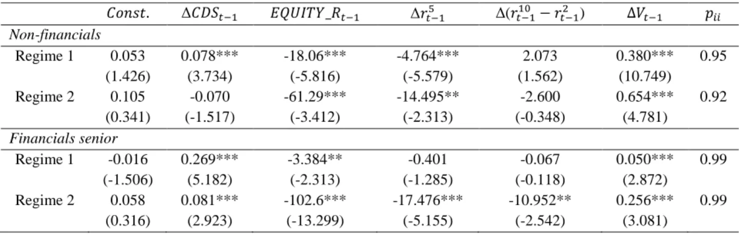
In Tables 3 and 4, we report coefficient estimates (and their significance), t-statistics (in parentheses) and

transition probabilities of the Markov switching models. Adjusted cannot be calculated in such

regime-switching models. However, note that the majority of the explanatory variables are highly significant in both regimes and for both indices. The probabilities of remaining in each regime are very

high, thus implying persistence. Interestingly, in the case of the non-financials iTraxx index, we find that

11

negative sign. This finding is supported by the estimate obtained from the structural model, which is significant at the 5% significance level. Hence, using a linear model, we would conclude that, contrary to previous findings, CDS spreads are negatively correlated. However, our sample period is clearly affected by different regimes of volatility in the CDS market. The outputs from the Markov switching models also suggest that CDS spreads are positively correlated in low volatility periods. However, when volatility is high, the autocorrelation becomes negative. In the period we analysed, which includes one of the worst crisis in the financial markets, the latter finding is probably due to the fact that credit investors sold off their CDS positions either to reap profits (if any) or to avoid further losses.

5. Out-of-sample statistical performance of the models

The analysis of the statistical performance of the forecasting models is based on the comparison between the point forecasts generated by each model and the actual values of the daily changes in CDS spreads. As stated in Section 2, we estimated the models over three different sample periods. This allows us to analyse three sets of daily point forecasts over three out-of-sample periods. In particular, the three out-of-sample periods are (1) from January 1, 2007 to September 15, 2010; (2) from January 1, 2008 to September 15, 2010; (3) from August 1, 2008 to September 15, 2010. In order to generate the daily forecasts, each model is estimated recursively.

We employ three main indicators to evaluate the statistical performance of each model’s forecasts, namely the root mean squared error (RMSE), the mean absolute error (MAE) and the mean correct prediction (MCP) of the direction of CDS spread changes. These forecasts are then compared with those obtained from the AR(1) model, which constitutes our benchmark model. We choose the AR(1) as a benchmark model because it has been used by Byström (2006), who found that it well describes the statistical features of iTraxx CDS spreads. Subsequently, we perform the modified Diebold and Mariano (1995) test (MDM, hereafter) for the RMSE and MAE indicators and a ratio test for the MCP indicator. These two statistical tests are used to test the null hypothesis that the model under consideration and the AR(1) have equal forecasting ability.

5.1 Description of the statistical tests

We now describe the main characteristics of these two tests. As we are performing pairwise comparisons of models’ forecasts, we have to define two series of forecasted changes in the iTraxx index price. The first one corresponds to the series of forecast changes generated by our benchmark model (the AR(1)

12

model) defined as ( ̂ )

. The second one is the series of forecast changes generated by model

i, where i corresponds to the model under consideration, which can be any of the remaining models we

estimated, namely the random walk, the structural model, the Markov switching structural model, the

Markov switching AR(1). This second series is defined as ( ̂ )

. The next step is to define, for

each of the two series of forecast changes, a loss function, namely ( ) and ( ) for the benchmark

model and the ith model under consideration, respectively. ( ) represents the forecast errors

between the benchmark model and the actual series of CDS spread changes. Similarly, ( ) represents

the forecast errors between the ith model under consideration and the actual series of CDS spread

changes. Finally, a loss differential in period t, defined as ( ) ( ), constitutes the basis for

our hypothesis testing. In particular, we test the null hypothesis ( ) for the MDM test, defined as

( ) , against the alternative hypothesis ( ) that ( ) . As we are performing one-step ahead forecasts, we use the test statistic suggested by Harvey et al. (1997):

 

var

i i i

d

MDM

d



(1.12) where ̅ ∑ and ( ̅ ) [ ∑ ] [ _{( )}

]. represents the sample

variance of the series, denotes the its ith autocovariance and h is the forecast horizon which is set

equal to 1 in our case.

As the value of ( ̅ ) has to be estimated, the test statistic in (1.12) follows a t-distribution with

( ) degrees of freedom.

As highlighted earlier, we also use a ratio test to analyse the statistical performance of the models in terms of the MCP indicator. Again, the null hypothesis to be tested is that the forecast errors from the benchmark model and the model under consideration are identical. The alternative hypothesis is that the given pair of models produces different forecast errors. In order to perform the test, we calculate the

following F-statistic: 1 1 n i t t n AR t t e F e   





(1.13)

13

If the null hypothesis is true, (1.13) follows a standard F-distribution with ( ) degrees of freedom. For

clarity, it is worth mentioning that the MCP cannot be calculated for the random walk model. In this case,

in order to be still able to compute the F-statistic, we follow Konstantinidi et al. (2008) and assign a value

of 50% for the MCP, based on the assumption that the possibility of having either a positive or negative forecast of CDS spread changes is equal to 50%.

5.2 Statistical predictability: results

Table 5 and Table 6 report the out-of-sample performance of the forecasting models for the

non-financials and financials senior CDS indices, respectively. Both tables report the values obtained for the RMSE, MAE and MCP, which are based on forecasts produced by the random walk model (Panel A), the structural model (Panel B), the AR(1) model (Panel C), the Markov switching structural model (Panel D) and the Markov switching AR(1) model (Panel E).

For both CDS indices, the tests clearly show that, based on the RMSE and MAE metrics, the random walk and the Markov switching structural model generate forecasts which are statistically different (at the 1% significance level) from the forecasts generated by our benchmark model, namely the AR(1) model. Interestingly, the structural model and the Markov switching AR(1) produce forecasts which are statistically equal to the AR(1) model. Thus, we can conclude that these two specifications are superior to both the random walk and the Markov switching structural model.

Based on these metrics and statistical tests, we find that there is supporting evidence of a statistically

predictable pattern in the evolution of the changes in spreads for both the non-financials and financials

senior CDS indices, even though results from the ratio test disagree.

6. The economic performance of the models

In the previous section, the results showed that there is some evidence of statistical predictability in the iTraxx CDS index spreads. For this reason, it is worth investigating this in more depth. In order to do that, we examine the economic significance of the models’ performance by creating trading strategies based on point forecasts.

6.1 The trading rules

In order to build trading strategies based on iTraxx index CDS spreads, we follow Byström (2006) and treat the CDS index spread as a corporate bond spread. We add the index spread to the risk-free interest

14

rate and use their sum to price a hypothetical 5-year zero coupon corporate bond with notional amount N

(arbitrarily chosen).6

We use the following trading rule:

If ( ) ( ) ̂ , then a trader would go short (long) a 5-year zero coupon bond;

otherwise, a trader would not make any trades and earn the risk-free interest rate instead. represents a

trading trigger defined by the trader. The use of a trading trigger is introduced in order to reduce the impact of transaction costs on the overall profitability of the strategies. In fact, the use of no (or low) triggers resulted in extremely negative returns in the similar study conducted by Byström (2006).

This trading rule is based on the fact that if the forecasted change in the CDS spread is considerably higher (lower) than the current spread, then the CDS index spread is expected to increase (decrease). The latter, in turn, would induce a contemporaneous decrease (increase) in the price of the zero coupon bond. Based on this prediction, a trader would sell (buy) the bond. Following Byström (2006), we assume that all trades are made either at the bid or ask prices, in order to include transaction costs when implementing the trading rule. Specifically, we buy at the ask price and we sell at the bid price.

We experiment the implementation of three different trading strategies, which are based on the same

trading rule. In particular, the first strategy uses a trading trigger which equals 1 basis point and a

holding period of one day. The second strategy explores a trading trigger of 2 basis points and a holding

period of one day. The third strategy does not use a trading trigger ( ) but is characterised by a

holding period of one week (5 days). The latter strategy draws on the finding of Blanco et al. (2005) about the average half-life of deviations between CDS spreads and credit spreads. They argue that spreads revert to equilibrium in approximately 6 days, on average. Even though their study is on individual credit obligors, they compute the average half-life of deviations across the pool of companies in their dataset. Our focus is on the iTraxx CDS index, which is a pool of companies with different credit risk characteristics. Hence, the comparison between our data sample and theirs is appropriate. By implementing this strategy, we then capture potential delays in the expected change in CDS spreads.

6

We are aware that iTraxx indices are not traded this way in the real world. However, ours represents a simple and accurate way to quantify the magnitude of profits that can be made from trading the index. In the real world, a trader willing to buy (sell) the index would have to pay (receive) a quarterly fixed coupon in addition to upfront payments made at initiation and close of the trade (to reflect the change in price of the index). Furthermore, he would have to account for any accrued interest between the launch of the index and the trade date. In order to compute upfront payments, the price of the index at the trade date has to be determined. This is given by the par minus the present value of the spread differences. Bloomberg provides a function, namely <CDSW>, which computes the index price for any level of spread and recovery rate assumptions.

15

6.2 Results on the profitability of the trading strategies

In Table 7 we report the annualised Sharpe ratios generated by the trading rules (described in the previous section) for each strategy over the three out-of-sample periods, namely January 2006 to September 2010, January 2008 to September 2010 and August 2008 to September 2010. The number of trades and the returns (expressed in percentages) of the strategies are also reported. In particular, results are shown for

both the non-financials and financials senior CDS indices for trading strategies based on forecasts

produced by the structural model (Panel A), the AR(1) model (Panel B), the Markov switching structural model (Panel C) and the Markov switching AR(1) model (Panel D).

In the case of the financials senior CDS index, we notice that the Sharpe ratios are negative most of the

times, except for three cases. However, for the non-financials iTraxx index, we observe positive Sharpe

ratios more frequently. In particular, the linear AR(1) model generates positive values over every out-of-sample period for strategies which require a trading trigger (of 1 or 2 basis points) and a daily holding period. In the latter case, holding positions for one week would result in highly negative returns and Sharpe ratios. On the other hand, a 1-week holding period would be beneficial for the structural model as positive returns and Sharpe ratios would be gained in 2 (out of 3) out-of-sample periods. The use of a high trading trigger (2 basis points) also generates positive Sharpe ratios for the Markov switching AR(1) model in all out-of-sample periods. The Markov switching structural model generates negative Sharpe ratios in every case.

Interestingly, the main conclusion we can draw from these results is that a AR(1) model seems to be best suited for higher frequency traders (with a trading horizon of 1 day), whereas a structural model seems more appropriate for traders with a longer holding period (1 week). An argument for this finding may relate to the fact that the iTraxx market takes longer than a day to adjust to new information embedded in the structural determinants of CDS spreads.

The fact that positive Sharpe ratios are found in some instances is not surprising and in line with our analysis in Section 5, where we analysed the statistical performance of the models and found that the random walk model generates worse forecasts than the AR(1), the structural model and the Markov switching AR(1) model. The trading strategies which are based on the latter models are indeed the only ones for which we observe some evidence of profitability.

16

7. Conclusion

Previous studies on the CDS market have predominantly focused on determining the economic factors that influence CDS spreads. To our knowledge, none of these studies have examined whether future CDS spreads are predictable using these economic determinants. This study aims to bridge that gap in the literature. Our paper is novel as it is the first to investigate whether it is possible to forecast CDS spreads using advanced econometric models. It is also the first study to evaluate trading strategies for CDS spreads using forecasts from robust econometric models.

We consider the most liquid CDS market in Europe, namely the iTraxx CDS index and focus on the

non-financials and financials senior iTraxx Europe indices. We employ both linear and non-linear forecasting models. In the former category we include the structural model and the AR(1) model, whereas in the latter we consider the Markov switching structural model and the Markov switching AR(1) model. Point forecasts based on each model are generated and their statistical and economic performance is assessed. Specifically, the statistical performance of the models is evaluated via the use of standard forecasting metrics (RMSE, MAE and MCP), while their economic performance is tested by implementing trading strategies based on iTraxx Europe CDS spreads. We find that the statistical analysis of the models is coherent with their trading results. In fact, the models which perform better from a statistical viewpoint - the structural model, the AR(1) model and the Markov switching AR(1) model - are also the models that generate positive returns and Sharpe ratios in some instances. Furthermore, the statistical and economic performances of the models are generally stable across the three sub-samples.

The trading strategies based on these models are better suited to be implemented for the non-financials

index, whereas they do not seem to generate positive profits for the financials senior index (except in

three occasions). Overall, we find that linear models outperform Markov switching models. The latter provide a good fit for iTraxx index data, but should not be used for forecasting purposes. Furthermore, among the linear models, autoregressive models should be preferred by traders with a shorter trading horizon (such as 1 day), whilst a structural model should be used by lower frequency traders (willing to hold their positions for at least 5 days). Another interesting finding relates to the existence of first-order autocorrelation in iTraxx Europe spreads. In low-volatility regimes, we find positive autocorrelation in CDS spreads, in line with previous studies which analysed the iTraxx index. However, in high-volatility states, the relationship is reversed. We are the first authors to document the presence of negative autocorrelation in iTraxx spreads and this is achieved through the use of a non-linear model such as the Markov switching model which allows us to distinguish between different states of the economy. This novel finding may be explained by the jittery reaction of credit investors who had been selling off their

17

CDS positions while the financial crisis was sluggishly unfolding. In conclusion, our findings show some evidence of predictability for the most liquid CDS index in Europe. As a result, the iTraxx index cannot be regarded as informationally efficient in its weak form altogether, and hence trading the index should be incentivised based on speculative reasons.

References

Alexander, C., Kaeck, A., 2008. Regime dependent determinants of credit default swap spreads. Journal of Banking and Finance 32, 1008-1021.

Benkert, C., 2004. Explaining credit default swap premia. Journal of Futures Markets 24, 71-92.

Berndt, A., Ostrovnaya, A., 2008. Do equity markets favour credit market news over options market news? Working Paper, Carnegie Mellon University.

Black, F., Cox, J., 1976. Valuing corporate securities: some effects of bond indenture provisions. Journal of Finance 31, 351-367.

Blanco, F., Brennan, S., Marsh, I.W., 2005. An empirical analysis of the dynamic relationship between investment grade bonds and credit default swaps. Journal of Finance 60, 2255-2281.

Byström, H., 2006. CreditGrades and the iTraxx CDS index market. Financial Analysts Journal 62, 65-76.

Campbell, J., Y., Taksler, G., B., 2003. Equity volatility and corporate bond yields. Journal of Finance 58, 2321-2350.

Cao, C., Yu, F., Zhong, Z., 2010. The information content of option-implied volatility for credit default swap valuation. Journal of Financial Markets 13, 321-343.

Collin-Dufresne, P., Goldstein, R.S., Martin, S.J., 2001. The Determinants of Credit Spread Changes. Journal of Finance 56, 2177-2207.

Cremers, M., Driessen, J., Maenhout, P., Weinbaum, D., 2008. Individual stock-option prices and credit spreads. Journal of Banking and Finance 32, 2706-2715.

Delianedis, G., Geske, R., 2001. The components of corporate credit spreads: default, recovery, tax, jumps, liquidity, and market factors. Working Paper 22-01, Anderson School, UCLA.

Dickey, D.A., Fuller, W.A., 1981. Likelihood ratio statistics for autoregressive time series with a unit root. Econometrica 49, 1057-1072.

Diebold, F.X., Mariano, R., 1995. Comparing predictive accuracy. Journal of Business and Economic Statistics 13, 253-265.

Driessen, J., 2005. Is default event risk priced in corporate bonds? Review of Financial Studies 18, 165-195.

18

Elton, E.J., Gruber, M.J., Agrawal, D., Mann, C., 2001. Explaining the rate spread on corporate bonds. Journal of Finance 56, 247-277.

Eom, Y., Helwege, J., Huang, J., 2004. Structural models of corporate bond pricing: an empirical analysis. Review of Financial Studies 17, 499-544.

Ericsson, J., Jacobs, K., Oviedo, R., 2009. The determinants of credit default swap premia. Journal of Financial and Quantitative Analysis 44, 109-132.

Forte, S., Peña, J.I., 2009. Credit spreads: An empirical analysis on the informational content of stocks, bonds, and CDS. Journal of Banking and Finance 33, 2013-2025.

Hamilton, J., 1994. Time series analysis. Princeton, NJ: Princess University Press.

Hamilton, J.D., Kim, D.H., 2000. A re-examination of the predictability of economic activity using the yield spread. NBER Working Paper Series, No. 7954.

Harvey, D.I., Leybourne, S.J., Newbold, P., 1997. Testing the equality of prediction mean squared errors. International Journal of Forecasting 13, 281-291.

Houweling, P., Vorst, T., 2005. Pricing default swaps: empirical evidence. Journal of International Money and Finance 24, 1200-1225.

Huang, J.Z., Huang, M., 2003. How much of corporate-treasury yield spread is due to credit risk?: a new calibration approach. Working Paper.

Jones, E.P., Mason, S.P., Rosenfeld, E., 1984. Contingent claims analysis of corporate capital structures: an empirical investigation. Journal of Finance 39, 611-625.

Konstantinidi, E., Skiadopolous, G., Tzagkaraki, E., 2008. Can the evolution of implied volatility be forecasted? Evidence from European and US implied volatility indices. Journal of Banking and Finance 33, 2401-2411.

Leland, H., 1994. Risky debt, bond covenants and optimal capital structure. Journal of Finance 49, 1213-1252.

Leland, H., Toft, K.B., 1996. Optimal capital structure, endogenous bankruptcy, and the term structure of credit spreads. Journal of Finance 51, 987-1019.

Longstaff, F.A., Mithal, S., Neis, E., 2003. The credit-default swap market: is credit protection priced correctly? Working Paper, UCLA.

Longstaff, F.A., Mithal, S., Neis, E., 2005. Corporate yield spreads: default risk or liquidity? New evidence from the credit default swap market. Journal of Finance 60, 2213-2253.

Longstaff, F.A., Schwartz E.S., 1995. A simple approach to valuing risky and floating rate debt. Journal of Finance 50, 789-819.

Merton, R., 1974. On the pricing of corporate debt: the risk structure of interest rates. Journal of Finance 29, 449-470.

19

Norden, L., Weber, M., 2009. The co-movement of credit default swap, bond and stock markets: an empirical analysis. European Financial Management 15, 529-562.

Zhang, B.Y., Zhou, H., Zhu, H., 2009. Explaining credit default swap spreads with the equity volatility and jump risks of individual firms. Review of Financial Studies 22, 5099-5131.

Zhu, H., 2004. An empirical comparison of credit spreads between the bond market and the credit default swap market. Journal of Financial Services Research 29, 211-235.

20

Table 1 – Summary statistics

This table reports the summary statistics for the variables used in our analysis over the whole sample

period. The CDS spreads for financials senior ( ) and non-financials ( ) represent our

dependent variables. The independent variables are the equally weighted portfolio of stocks comprising

the same members of the CDS indices ( and , respectively for the financials senior

and non-financials sub-indices), the level of the risk-free interest rate ( ), the slope of the yield curve

( ), the VStoxx implied volatility index ( ).

Mean Std dev Skewness Kurtosis Bera-Jarque ADF

Panel A: Summary statistics for variables levels

66.3248 51.6708 0.4058 2.0293 82.3810*** 0.995*** -1.3380 75.2712 48.6125 1.3794 4.4303 455.0609*** 0.995*** -1.6024 51.4140 13.0064 -0.2197 1.9327 68.5568*** 0.997*** -1.2447 141.5066 39.2978 1.2829 3.3404 315.6771*** 0.995*** 0.3853 0.0357 0.0086 -0.1736 1.8902 69.5890*** 0.997*** -0.3415 0.0074 0.0071 0.4239 1.6361 132.7035*** 0.999*** -0.8494 25.5701 11.3994 1.7470 6.8192 1378.780*** 0.982*** -2.4886

Panel B: Summary statistics for variables changes

0.1017 4.9137 -0.4666 18.1176 13678.71*** 0.127*** -22.5877*** 0.0498 4.9078 6.8367 149.9050 1024912*** -0.042 -9.5454*** 0.0002 0.0227 0.2790 12.6447 5564.893*** 0.052* -9.2523*** 0.0008 0.0183 1.4473 48.4918 97833.63*** 0.006 -21.2677*** 0.0000 0.0005 0.0512 4.7944 192.6095*** -0.029 -38.9321*** 0.0000 0.0003 -0.1667 8.5259 1827.321*** 0.094*** -8.2833*** 0.0039 2.0699 1.8298 29.0801 41353.68*** -0.041 -11.8205***

21

Table 2 - Parameter estimates for Structural Model and AR(1)

Estimated parameters, over the whole sample, for the OLS regressions of changes in European iTraxx CDS indices on lagged theoretical determinants of CDS spreads (as defined in equation 1.1) and on lagged CDS spreads (as defined in equation 1.2) are shown in Panel A and B, respectively. Standard

t-statistics are given within brackets. Adjusted are reported in the last column.

Δ Δ Δ( )

Panel A: Structural Model

Non-financials 0.069 (0.472) -0.073** (-2.247) -19.984** (-2.041) -1.319 (-0.428) -8.794** (-2.265) 0.022 (0.266) 0.008 Financials senior 0.073 (0.532) 0.140*** (3.966) -9.723 (-1.165) -10.653*** (-3.433) 0.051 (0.012) -0.389*** (-4.717) 0.039 Panel B: AR(1) Non-financials 0.050 (0.340) -0.042 (-1.423) - - - - 0.001 Financials senior 0.076 (0.550) 0.123*** (4.361) - - - - 0.014

22

Table 3 – Parameter estimates for Markov Switching Structural Model

Estimated parameters, over the whole sample, for the Markov switching regressions of changes in European iTraxx CDS indices on lagged theoretical determinants of CDS spreads (as defined in equation 1.3). Standard t-statistics are given within parentheses.

Δ Δ Δ( ) Non-financials Regime 1 0.053 (1.426) 0.078*** (3.734) -18.06*** (-5.816) -4.764*** (-5.579) 2.073 (1.562) 0.380*** (10.749) 0.95 Regime 2 0.105 (0.341) -0.070 (-1.517) -61.29*** (-3.412) -14.495** (-2.313) -2.600 (-0.348) 0.654*** (4.781) 0.92 Financials senior Regime 1 -0.016 (-1.506) 0.269*** (5.182) -3.384** (-2.313) -0.401 (-1.285) -0.067 (-0.118) 0.050*** (2.872) 0.99 Regime 2 0.058 (0.316) 0.081*** (2.923) -102.6*** (-13.299) -17.476*** (-5.155) -10.952** (-2.542) 0.256*** (3.081) 0.99

*, **, *** indicate rejection of the null hypothesis at the 10%, 5% and 1%, respectively.

Table 4 – Parameter estimates for Markov Switching AR(1)

Estimated parameters, over the whole sample, for the Markov switching regressions of changes in European iTraxx CDS indices on lagged CDS spreads (as defined in equation 1.9). Standard t-statistics are given within brackets.

Δ Non-financials Regime 1 0.0283 (0.204) 0.1525*** (5.117) 0.98 Regime 2 -0.0167 (-0.423) -0.581 (1.000) 0.98 Financials senior Regime 1 0.077 (0.432) 0.258*** (2.830) 0.99 Regime 2 -0.071 (-0.231) 0.162*** (4.211) 0.99

23

Table 5 – Out-of-sample performance of the forecasting models for the non-financials CDS index

This table presents the out-of-sample performance of each model for the non-financials CDS index. We

report the root mean squared error (RMSE), the mean absolute error (MAE) and the mean correct prediction (MCP) of the sign of the CDS spread change. We generated forecasts by implementing the random walk model (Panel A), the structural model (Panel B), the AR(1) model (Panel C), the Markov switching structural model (Panel D) and the Markov switching AR(1) model (Panel E). In order to test the null hypothesis that the AR(1) model and the model under consideration generate equal forecasts, we perform the Modified Diebold-Mariano test (for RMSE and MAE) and the ratio test (for MCP). We estimated the models recursively for three different sample periods: January 2007 to September 15, 2010; January 2008 to September 15, 2010 and August 2008 to September 15, 2010.

Jan 2007 – Sep 2010 Jan 2008 – Sep 2010 Aug 2008 – Sep 2010

Non-financials:

Panel A: Random Walk

RMSE 8.24*** 9.49*** 9.18***

MAE 4.17*** 5.14*** 4.88***

Panel B: Structural Model

RMSE 5.74* 6.59* 6.49* MAE 2.95* 3.60* 3.43* MCP (%) 48.14 48.76 48.69 Panel C: AR(1) RMSE 5.72 6.57 6.46 MAE 2.92 3.56 3.39 MCP (%) 47.54 47.94 48.29

Panel D: Markov Switching Structural Model

RMSE 5.85*** 6.63*** 6.52***

MAE 3.06*** 3.68*** 3.50***

MCP (%) 47.90 48.43 48.69

Panel E: Markov Switching AR(1)

RMSE 5.72 6.56 6.45

MAE 2.93 3.57 3.39

MCP (%) 48.62 48.27 48.69

24

Table 6 – Out-of-sample performance of the forecasting models for the financials senior CDS index

This table presents the out-of-sample performance of each model for the financials senior CDS index. We

report the root mean squared error (RMSE), the mean absolute error (MAE) and the mean correct prediction (MCP) of the sign of the CDS spread change. We generated forecasts by implementing the random walk model (Panel A), the structural model (Panel B), the AR(1) model (Panel C), the Markov switching structural model (Panel D) and the Markov switching AR(1) model (Panel E). In order to test the null hypothesis that the AR(1) model and the model under consideration generate equal forecasts, we perform the Modified Diebold-Mariano test (for RMSE and MAE) and the ratio test (for MCP). We estimated the models recursively for three different sample periods: January 2007 to September 15, 2010; January 2008 to September 15, 2010 and August 2008 to September 15, 2010.

Jan 2007 – Sep 2010 Jan 2008 – Sep 2010 Aug 2008 – Sep 2010

Financials senior:

Panel A: Random Walk

RMSE 7.50*** 8.52*** 8.33***

MAE 4.72*** 5.82*** 5.66***

Panel B: Structural Model

RMSE 5.79 6.53 6.50 MAE 3.60 4.42 4.31 MCP (%) 51.80 50.82 51.53 Panel C: AR(1) RMSE 5.79 6.54 6.53 MAE 3.59 4.40 4.33 MCP (%) 50.38 49.03 47.90

Panel D: Markov Switching Structural Model

RMSE 6.22*** 6.67*** 6.63

MAE 3.75*** 4.51*** 4.38

MCP (%) 50.60 49.63 50.00

Panel E: Markov Switching AR(1)

RMSE 5.96 6.55 6.54

MAE 3.62 4.41 4.33

MCP (%) 49.84 48.73 47.90

25

Table 7 – Profitability of trading strategies based on the models’ forecasts

We implement trading strategies on the non-financials and financials senior CDS indices, which are

based on point forecasts obtained from the structural model (Panel A), the AR(1) model (Panel B), the Markov switching structural model (Panel C) and the Markov switching AR(1) model (Panel D). For each strategy, we report the number of trades, the returns over the out-of-sample period and the annualised Sharpe ratio.

Threshold Jan 2007 – Sep 2010 Jan 2008 – Sep 2010 Aug 2008 – Sep 2010

Trades Return (%) Sharpe Trades Return (%) Sharpe Trades Return (%) Sharpe Non-financials:

Panel A: Structural Model

+/- 1bp 76 9.52 -0.12 71 5.31 -0.13 57 2.07 -0.39 +/- 2bp 13 9.96 -0.12 11 5.79 -0.10 8 3.62 -0.10 Hold 1week 167 -0.18 -0.23 122 4.25 0.62 100 6.18 1.27 Panel B: AR(1) +/- 1bp 20 12.23 0.43 15 7.92 0.55 6 4.83 0.47 +/- 2bp 6 11.46 0.38 4 7.23 0.54 1 5.17 0.71 Hold 1week 167 -21.05 -3.40 122 -22.86 -5.31 100 -20.20 -5.67

Panel C: Markov Switching Structural Model

+/- 1bp 118 4.60 -0.70 107 0.07 -0.90 86 -2.16 -1.11 +/- 2bp 18 9.76 -0.17 31 2.65 -0.93 21 0.97 -0.92 Hold 1week 167 -7.91 -1.30 122 -4.91 -1.12 100 -5.62 -1.47

Panel D: Markov Switching AR(1)

+/- 1bp 28 6.27 -1.03 24 2.54 -1.10 14 1.98 -0.76 +/- 2bp 8 10.55 0.03 6 6.48 0.15 2 5.02 0.62 Hold 1week 167 -15.04 -2.38 122 -13.63 -2.98 100 -16.82 -4.56

Financials senior:

Panel A: Structural Model

+/- 1bp 171 7.67 -0.52 159 3.76 -0.55 111 4.47 -0.23 +/- 2bp 48 11.23 -0.33 45 7.19 -0.28 37 6.89 0.15 Hold 1week 183 3.89 0.21 134 -9.30 -1.72 105 -9.44 -2.14 Panel B: AR(1) +/- 1bp 90 9.62 -0.41 84 5.10 -0.48 72 2.93 -0.50 +/- 2bp 16 10.50 -0.46 13 6.49 -0.44 10 5.20 -0.21 Hold 1week 183 2.66 0.06 134 1.06 -0.04 105 -0.96 -0.36

Panel C: Markov Switching Structural Model

+/- 1bp 255 -0.41 -1.10 213 -0.14 -0.87 140 0.83 -0.69 +/- 2bp 97 7.31 -0.70 83 4.54 -0.59 51 4.67 -0.27 Hold 1week 183 -1.83 -0.52 134 -11.55 -2.11 105 -9.53 -2.16

Panel D: Markov Switching AR(1)

+/- 1bp 105 7.10 -0.65 92 3.83 -0.62 79 0.24 -0.89 +/- 2bp 21 9.39 -0.62 15 5.75 -0.57 12 3.67 -0.52 Hold 1week 183 0.10 -0.27 134 -6.34 -1.22 105 -4.58 -1.10