Having a Blast: Meta-Learning and Heterogeneous Ensembles for Data Streams

Having a Blast: Meta-Learning and

Heterogeneous Ensembles for Data Streams

Jan N. van Rijn

, Geoffrey Holmes

, Bernhard Pfahringer

and Joaquin Vanschoren

Abstract—Ensembles of classifiers are among the best per-forming classifiers available in many data mining applications. However, most ensembles developed specifically for the dynamic data stream setting rely on only one type of base-level classifier, most often Hoeffding Trees. In this paper, we study the use of heterogeneous ensembles, comprised of fundamentally different model types. Heterogeneous ensembles have proven successful in the classical batch data setting, however they do not easily transfer to the data stream setting. We therefore introduce the Online Performance Estimation framework, which can be used in data stream ensembles to weight the votes of (heterogeneous) ensemble members differently across the stream. Experiments over a wide range of data streams show performance that is competitive with state of the art ensemble techniques, including Online Bagging and Leveraging Bagging. All experimental results from this work are easily reproducible and publicly available on OpenML for further analysis.

I. INTRODUCTION

Real-time analysis of data streams has become a key area of data mining research [1]. The research community has developed a large number of machine learning algorithms capable of modelling general trends in stream data and make accurate predictions for future observations. In many applica-tions,ensemblesof classifiers are the most accurate classifiers available. Rather than building one model, a variety of models are generated that all vote for a certain class label.

One way to vastly improve the performance of ensembles is to build heterogeneous ensembles, consisting of models generated by very different techniques, rather than homoge-neous ensembles, in which all models are generated by the same technique. One technique to build such a heterogeneous ensemble is Stacking [2], which has been extensively analysed in classical batch data mining applications. As the underlying techniques upon which Stacking relies can not be trivially transferred to the data stream setting, there are few successful heterogeneous ensemble techniques in the data stream setting. Most approaches rely on meta-learning [3], [4]. This requires the extraction of computationally expensive meta-features, yet it yields marginal improvements.

In this work we introduce a more elegant technique that natively allows heterogeneous model combination in the data stream setting. It weights the votes of the ensemble members based on their performance on recent observations. It is inspired by Online Boosting [5] and Accuracy Weighted Ensembles [6], which rely on a similar tech-nique, but are both fundamentally different. Moreover, al-though both ensemble techniques slightly improve the accuracy

of their base-classifiers, neither are considered competitive with state of the art techniques [5].

Our contributions are the following. We define Online Performance Estimation, a framework that provides dynamic

weighting of the votes of individual ensemble members across the stream. Utilizing this framework, we introduce a new ensemble technique that combines heterogeneous models. We conduct an extensive empirical study, covering62data streams, that shows that this technique is competitive with state of the art ensembles, and superior to meta-learning approaches.

II. RELATEDWORK

It has been recognized that data stream mining differs significantly from conventional batch data mining [1], [7], [8], [9]. In the conventional batch setting, a finite amount of stationary data is provided and the goal is to build a model that fits the data as well as possible. When working with data streams, we should expect an infinite amount of data, where observations come in one by one and are being processed in that order. Furthermore, the nature of the data can change over time, a notion known as concept drift. Classifiers should be able to detect when a learned model becomes obsolete and update it.

Common Approaches. Some batch classifiers can be trivially adapted to a data stream setting. Examples are k Nearest Neighbour[10],Stochastic Gradient Descent [11] and SPegasos (short for: Stochastic Pri-mal Estimated sub-GrAdient SOlver for SVM) [12]. Both

Stochastic Gradient Descent and SPegasos are gradient descent methods, capable of learning a variety of linear models, such as Support Vector Machines and Logistic Regression.

Other classifiers have been created specifically to oper-ate on data streams. Most notably, the Hoeffding Tree

induction algorithm [13] inspects every example only once, and stores per-leaf statistics to calculate the information gain

on which the split criterion is determined. The Hoeffding bound states that the true mean of a random variable of a given range will not differ from the estimated mean by more than a certain value, and this provides statistical evidence that a certain split is superior over others. As Hoeffding Trees seem to work very well in practice, many vari-ants have been proposed, such as Random Hoeffding Trees,Adaptive Hoeffding TreesandHoeffding Option Trees[14].

Finally, a commonly used technique to adapt traditional batch classifiers to the stream setting is training them on a window of w recent examples: after w new examples have been observed, a new model is built. This approach has the advantage that old examples are ignored, providing natural protection against concept drift. A disadvantage is that it rarely operates on the most recently data. Read et al. [1] compare the performance of these batch-incremental classifiers with common data stream classifiers, and conclude that the over-all performance is equivalent, although the batch-incremental classifiers generally use more resources (time and memory).

Ensembles.Ensemble techniques train multiple classifiers on a set of weighted training examples, and these weights can vary for different classifiers. In order to classify test examples, all individual models produce a prediction, also called a vote, and the final prediction is made according to a predefined voting schema, e.g., the class with the most votes is selected. Bagging [15] exploits the instability of classifiers by training them on different bootstrap replicates: resamplings (with replacement) of the training set. Effectively, the training sets for various classifiers differ by the weights of their training examples. Online Bagging [5] operates on data streams by drawing the weight of each example from a Poisson distribution, which converges to the behavior of the classical Bagging algorithm if the number of examples is large. Boosting [16] is a technique that sequentially trains multiple classifiers, in which more weight is given to exam-ples that were misclassified by earlier classifiers. Online Boosting [5] applies this technique on data streams by assigning more weight to training examples that were mis-classified by previously trained classifiers in the ensemble. The Accuracy Weighted Ensemble [6] works well in combination with batch-incremental classifiers. It maintains multiple recent models trained on different batches of the data stream, and weights the votes of each model based on the expected predictive accuracy. Stacking [2] combines heterogeneous models in the classical batch setting. It weights the votes of the individual models based on a cross-validation procedure. As cross-validation procedures are not suitable for the data stream setting, no online version of Stacking exists. To the best of our knowledge, the only case of heterogeneous ensembles in the data stream setting is [17]. A combination of feature selection and heterogeneous ensembles is proposed; ensemble members that performed poorly can be replaced.

Concept drift.Some of the aforementioned methods nat-urally deal with concept drift. For instance, k Nearest Neighbour maintains a number of w recent examples, substituting each example after w new examples have been observed. Change detectors, such as Drift Detection Method (DDM) [18] and Adaptive Sliding Window Algorithm (ADWIN) [19] are stand-alone techniques that detect concept drift and can be used in combination with any stream classifier. Both rely on the assumption that classifiers improve (or at least maintain) their accuracy when trained on more data. When the accuracy of a classifier drops in respect to a reference window, this could mean that the learned concept is outdated, and a new classifier should be built. The main difference between DDM and ADWIN is the way they select the reference window. Furthermore, classifiers can have built-in drift detectors. For built-instance, Ultra Fast Forest of Trees[20] are Hoeffding Trees with a built-in change

detector for every node. When an earlier made split turns out to be obsolete, a new split can be generated.

Evaluation. As data from streams is non-stationary, the well-known cross-validation procedure for estimating model performance is not suitable. A commonly accepted estimation procedure is thePrequential Method[9], in which each example is first used to test the current model, and afterwards (either directly or after a delay) becomes available for training.

Meta-Learning. Meta-learning aims to learn which learn-ing techniques work well on what data. A common task, known as the Algorithm Selection Problem, is to determine which classifier performs best on a given dataset. We can predict this by training a meta-model on data describing the performance of different methods on different datasets, characterized by

meta-features[21]. Meta-learning approaches on data streams often train multiple classifiers on all available training data. A meta-model decides for each new data point which of the base-learners will make a prediction. The authors of [4] dynamically choose between two regression techniques using meta-knowledge obtained earlier in the stream. The authors of [3] select the best classifier among multiple classifiers, based on meta-knowledge from previously processed data streams. Finally, [22] uses meta-learning on time series with recurrent concepts: when concept drift is detected, a meta-learning algorithm decides whether a model trained previously on the same stream could be reused, or whether the data is so different from before that a new model must be trained.

III. METHODS

Traditional Machine Learning problems consist of a num-ber of examples that are observed in arbitrary order. Each example e = (x, l(x)) is a tuple of p predictive attributes

x= (x1, . . . , xp) and a target attributel(x). A data set is an

(unordered) set of such examples. The goal is to approximate a labelling function l : x → l(x). In the data stream setting the examples are observed in a given order, therefore each data stream S is a sequence of examplesS = (e1, e2, e3, . . . , en),

wherenis possibly infinite. Consequently,Sirefers to theith

example in data stream S. The set of predictive attributes of that example is denoted byPSi, likewisel(PSi)maps to the

corresponding label. Furthermore, the labelling function that needs to be learned can change over time due to concept drift. The ensemble method that we propose consists of funda-mentally different base-classifiers; Section IV describes which classifiers we use. These are trained using all available train-ing examples. At various points in the stream, we need to determine the weights of the ensemble members. As such, we are repeatedly dealing with the algorithm selection problem as we pass over the stream. Hence, meta-learning and ensemble techniques are closely related in the data stream setting. In order to address the online algorithm selection problem, we propose Online Performance Estimation.

A. Online Performance Estimation

When applying an ensemble, the most relevant variables are which base-classifiers (members) to use and how to weight their individual votes. The Online Performance Estimation framework addresses the latter question. In most common ap-proaches all base-classifiers are given the same weight (e.g., as

done in Bagging) or their predictions are otherwise combined to optimise the overall performance of the ensemble (e.g., as done in Stacking). An important property of the data stream setting has not been taken into account: due to the possible occurrence of concept drift it is likely that in most cases recent examples are more relevant than older ones. Moreover, due to the fact that there is a temporal component in both the training and test set, we can actually measure how ensemble members have performed on recent examples, and accordingly adjust their weight in the voting. In order to estimate the performance of a classifier on recent data, we calculate:

P(l0, c, w, L) = c X i=min(1,c−w) L(l0(PSi), l(PSi)) w (1)

where l0 is the learned labelling function of an ensemble member, c is the index of the last seen training example and w is the number of training examples over which we want to estimate the performance of ensemble members. Finally,L is a loss function that compares the labels predicted by the ensemble member to the true labels. The most simple version is a zero/one loss function, which returns 1 when the pre-dicted label is correct and0otherwise. More complicated loss functions can also be incorporated. Finally, the performance estimates for the ensemble members can be converted into a weight for their votes, at various points over the stream. For instance, the best performing members at that point could receive the highest weights.

Note that in order to apply Performance Estimation over a window of w examples, the meta-algorithm needs to store the most recent w examples in memory. However, under the assumption that parameterwis fixed a priori and that we only need to update the ensemble weights at predefined intervals (e.g., a fixed interval of length α), any ensemble technique can trivially be adapted to update its member’s weights under this framework, without having to revisit data points more than once. The choice of weighting function and ensemble technique can give rise to different algorithms, of which we will discuss several below.

B. BLAST

BLAST (short for best last) is an ensemble embodying Online Performance Estimation. For every set of αtest exam-ples, it selects one of its members to be the active classifier. The weight of the vote of the active classifier will be 1, while the weights of all other members are 0. The active classifier is selected using Online Performance Estimation: the classifier that performed best over the set of w previous trainings examples is selected as the active classifier, hence the name. Formally,

AC = arg max

mi∈M

P(mi, c, w, E) (2)

where M is the set of models generated by the ensemble members, c is the index of the current example, w is a parameter to be set by the user (the window size over which we do the performance estimation) and E is a zero/one loss function, giving a penalty of 1 to all misclassified examples.

The Online Performance Estimation framework contains some parameters to be determined by the user. As for the interval that the active classifier remains the same, a value of α= 1seems optimal, as the decision on what active classifier to use is always based on the performance evaluations on the most recent data. The optimal value for w is harder to determine. Setting this value too high will result in selecting the active classifier over possibly outdated data. Setting it too low will result in selecting the active classifier based on an unrepresentative sample. Furthermore, a loss function needs to be selected. In our experiments we have explicitly selected a zero/one loss function, as openly available data streams typically lack information about the costs of various types of misclassifications. However, when the appropriate domain knowledge is available, different loss functions can be chosen. Note that BLAST is not the first ensemble technique to utilize Online Performance Estimation. For example, the

Accuracy Weighted Ensemble and the Heterogeneous Ensemble technique from [17] replace outdated models based on measurable performance. The main contribution ofBLAST

is that it solely relies on Online Performance Estimation. Without introducing additional techniques or pre-processing steps we are able to measure the utility of Online Perfor-mance Estimation for Data Stream Ensembles. Furthermore, rather than replacing ensemble members, BLASTtemporarily lowers the weight of poorly performing members. This saves resources that are otherwise used for training new members.

C. Meta-Feature Ensemble

Several notable techniques for heterogeneous model com-bination in the data stream setting rely on meta-learning [3], [4]. These techniques divide the data stream in windows of size w. Over each of these windows, a set of meta-features is calculated, and this is repeated for all previously known data streams. Using these meta-features and the actual performances of all classifiers on all windows, a meta-classifier is trained to predict the best classifier for thenextwindow given the meta-features of the current window. Any batch classifier can be used as the meta-classifier. Usually, Random Forest [23] are used, since these have proven to work well in the context of algorithm selection [24]. We include this meta-learning approach in our study for two reasons. First, it can serve as a very strong baseline to compare against. Second, Online Performance Estimation can trivially be combined with this technique, raising some interesting research questions about its future potential. Section IV-C contains an experiment that strongly suggests that incorporating Online Performance Esti-mation increases the predictive performance of meta-learning techniques.

The performance of this technique highly depends on the meta-features that are used. We implemented the commonly used simple, statistical, information theoretic and landmarking meta-features [21], [24]. Additionally, we use concept drift detection features, first introduced in [3]. These meta-features describe the number of times a change detector (e.g.,

ADWIN or DDM) has measured concept drift in the previous window of w examples. The assumption is that when there is abrupt concept drift, fast learners (needing few examples to build adequate models) should be able to more quickly recover from this and give more accurate predictions [3], [25].

Furthermore, the estimated performance of each ensemble member can also be added as a meta-feature. We refer to this new kind of meta-feature as stream-based landmarkers. Additionally, we include a derived meta-feature ‘best on pre-vious’ that simply records which base-classifier performed best on the previous wexamples. Finally, for each base-classifier, we record a binary meta-feature indicating whether there was a significant difference between that classifier and the best classifier on that window, measured using McNemar’s test [9]. Note that the meta-classifier is trained on all previously seen data streams. Therefore, the quality of this method de-pends on the diversity of these streams. In this work, we do not train the meta-classifier on historic meta-data from the stream, as this requires the meta-classifier to retrain after each window, increasing runtime. Still, this means that potentially useful meta-information about performance earlier in the stream is neglected. We aim to explore this in future work.

IV. EXPERIMENTS

In order to establish the utility of Online Performance Estimation, we conduct experiments using a large set of data streams. The data streams and results of all experiments are made publicly available on OpenML [26] for the purposes of verifiability, reproducibility and generalizability.1

A. Setup

Data streams.The data streams are a combination of real world data streams (e.g., electricity, 20 newsgroups, IMDB) and synthetically generated data (e.g., LED, Rotating Hyper-plane, Bayesian Network Generator) commonly used in data stream research [1], [3], [7], [10]. Many contain a natural drift of concept. We estimate the performance of the methods using the Prequential Method: each observation is used as a test example first and as a training example afterwards [9].

Meta-classifier. The Meta-Feature Ensemble re-quires a meta-classifier that is trained on previously seen data streams. In this work, we use a Random Forest[23] consisting of 100 trees, as implemented in Weka3.7.12[27]. We evaluate the meta-classifier using a method similar to leave one out: for each data stream to test, we train the meta-classifier on all other data streams. However, data streams that are generated by the same data-generator can potentially be similar, resulting in an optimistic score. Therefore we remove those from the training set as well, except for data streams generated by the Bayesian Network Generator, as these can be considered very different by nature. Furthermore, some data streams are composed of other data streams. For instance, Covertype, Pokerhand and Electricity are commonly joined to form one data stream [1], [3], [8]. Hence, these will also be removed from each other’s training sets.

Ensembles.The most important property of heterogeneous ensembles is which base-classifiers are used. This affects both performance and runtime. Table I lists all classifiers that are used as base-classifiers in this paper. These are basically all classifiers that are available in the MOA workbench that can handle multi-nominal classification problems [7]. For most parameters the defaults of MOA version 2014.03 are used; k-NN has a window size of1,000 andk= 10.

1_{See http://www.openml.org/}

TABLE I. CLASSIFIERS USED IN THE EXPERIMENTS.

Key Classifier Model type

NB Naive Bayes Bayesian

SGD-Hinge Stochastic Gradient Descent / Hinge SVM

SGD-Log Stochastic Gradient Descent / Log Logistic

SPeg SPegasos / Hinge SVM

k-NN kNearest Neighbour Lazy

RC Rule Classifier Classification Rules

HT Hoeffding Tree Decision Tree

AT Hoeffding Adaptive Tree Decision Tree

RT Random Hoeffding Tree Decision Tree

OT Hoeffding Option Tree Option Tree

Perc Perceptron Neural Network

Evaluation.We evaluate the performance of the proposed methods in a way similar to [3], [4]:Base-level accuracyand

Meta-level accuracy. Base-level accuracy is the conventional predictive accuracy of the techniques on the task of labeling the test instances of the data streams, i.e., the number of correct predictions divided by the total number of predictions. This measure can be used to compare the performance of the proposed techniques to conventional ensemble techniques. Meta-level accuracy measures the accuracy obtained on the task of selecting the best active classifier on a window of test examples. This can be used to estimate how well the meta-classifier worked compared to other classifier selection schemas.

A low meta-level accuracy does not imply a low base-level accuracy. Meta-level accuracy does not capture the ranking of the base-classifiers and the individual differences in perfor-mance between them. For example, when two of the base-classifiers perform about as well, the meta-classifier suffices to select either one. However, meta-level accuracy can only be calculated for ensemble techniques that select a single active classifier. For these reasons, base-level accuracy always takes precedence when comparing techniques.

Parameters.Apart from the chosen set of base-classifiers, two important parameters need to be determined for BLAST

and the Meta-Feature Ensemble, i.e., the window size over which we do Online Performance Estimation (w) and the number of examples the active classifier is fixed (α). Even though it is plausible that an optimal value for α = 1, there are reasons not to chose this. It is computationally expensive to revise the weights after every example, especially for the

Meta-Feature Ensemble. Furthermore, for calculating meta-level accuracy it is beneficial to have α = w, so that all examples contribute equally to the meta-level task, and are used exactly once. For bothBLASTand theMeta-Feature Ensemblewe set parametersα=w= 1,000. Hence, the past

1,000example are used to define the weights of the ensemble members for the following window of1,000 examples.

Baselines.We compare the results of the defined methods with the Best Single Classifier. Each heterogeneous ensemble consists of n base-classifiers. For each of the data streams, the one that performs best on average over all other data streams is considered the best single classifier. Although it seems obvious that the proposed techniques perform better than this baseline, adopting this technique makes it possible to analyse the increase of both meta-level accuracy and base-level accuracy. Secondly, we also compare the obtained base-level accuracy with state of the art homogeneous ensembles, such as

TABLE II. PERFORMANCES AVERAGED OVER ALL DATA STREAMS.

Technique Meta-level acc. Base-level acc.

Majority Vote Ensemble N/A 0.814

Best Single 0.345 0.821

Online Boosting /HT N/A 0.822

Online Bagging /HT N/A 0.830

Leveraging Bagging /HT N/A 0.838

Meta-Feature Ensemble 0.526 0.848

BLAST 0.642 0.857

Oracle 1.000 0.861

as the Majority Vote Ensemble. The latter is a heterogeneous ensemble consisting of a set of n given base-classifiers, in which all base-classifiers vote equally for the class label. Fi-nally, an interesting measure to compare to is theOracle meta-classifier. This is a hypothetical meta-classifier that selects for every interval of α test-instances the best base-classifier out of a given set. Note that the base-level score obtained by the

Oracleindicates the maximal achievable score for the other techniques when using this set of base-classifiers. Therefore, it also gives a measure of how well the set of base-classifiers was designed; when the base-level accuracy of the Oracle

is only slightly better than the base-level accuracy of the best single classifier, this is an indication that the selected set of base-classifiers was not well chosen.

B. Ensemble Performance

In order to assess whether Online Performance Estimation is a useful technique, we run all techniques over the full range of data streams. Table II shows the results of the techniques averaged over all data streams. Note that the meta-level accuracy can only be measured for techniques that deal with an algorithm selection problem. The results show that

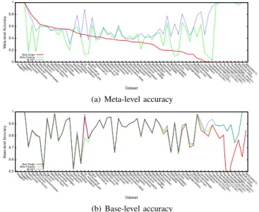
BLAST performs better than the other techniques, on both meta-level and base-level accuracy. Another important obser-vation is that the Majority Vote Ensemble performs poorly. In many cases it is not able to outperform the Best Single Classifier. This observation supports the notion that constructing an ensemble of heterogeneous models is not a trivial task, and proper techniques for weighting the individual votes are required. Figure 1 shows the performances of the techniques per data stream. Preventing to clutter the figures, we only show the three techniques for which we can measure meta-level performance. The data streams are sorted by the meta-level performance of the Best Single Classifier. It shows that BLAST performs consistently very well on most tasks. In almost all cases it outperforms the Meta-Feature Ensemble. This supports the notion that Online Performance Estimation is very suitable for deter-mining the best classifier on a part of a data stream.

To assess statistical significance, we use the Friedman test with post-hoc Nemenyi test to establish the statistical relevance of our results. These tests are considered the state of the art when it comes to comparing multiple classifiers [28]. The Friedman test checks whether there is a statistical difference between the classifiers; when this is the case the Nemenyi test can be used to determine which classifiers are significantly better than others. The results of the Nemenyi test are shown in Figure 2. It plots the average rank of all methods and the critical difference. Classifiers that are statistically equivalent are connected by a black line. For all other cases, there was a

0 0.2 0.4 0.6 0.8 1

Stagger3Stagger1Stagger2BNG(vowel)BNG(mfeat-fourier)BNG(sonar)BNG(JapaneseVowels)BNG(cmc)Agrawal1BNG(solar-flare)BNG(mushroom)pokerhandBNG(pendigits)BNG(zoo)codrnaNormBNG(letter)CovPokElecBNG(eucalyptus)20_newsgroups.driftBNG(credit-g)adultBNG(credit-a)BNG(wine)BNG(segment)BNG(kr-vs-kp)BNG(vote)BNG(vehicle)BNG(anneal)BNG(heart-c)BNG(waveform-5000)BNG(lymph)BNG(hepatitis)BNG(ionosphere)AirlinesCodrnaAdultBNG(trains)BNG(heart-statlog)BNG(satimage)BNG(labor)BNG(soybean)electricitySEA(50000)BNG(spambase)BNG(optdigits)airlinesSEA(50)BNG(page-blocks)LED(50000)BNG(tic-tac-toe)BNG(dermatology)covertypevehicleNormHyperplane(10;0.001)Hyperplane(10;0.0001)RandomRBF(0;0)RandomRBF(10;0.001)RandomRBF(10;0.0001)RandomRBF(50;0.001)RandomRBF(50;0.0001)BNG(bridges_version1)BNG(colic.ORIG)IMDB.dramaBNG(SPECT)

Meta-level Accuracy

Dataset

Best Single Meta-Feature BLAST

(a) Meta-level accuracy

0.5 0.6 0.7 0.8 0.9 1

Stagger3Stagger1Stagger2BNG(vowel)BNG(mfeat-fourier)BNG(sonar)BNG(JapaneseVowels)BNG(cmc)Agrawal1BNG(solar-flare)BNG(mushroom)pokerhandBNG(pendigits)BNG(zoo)codrnaNormBNG(letter)CovPokElecBNG(eucalyptus)20_newsgroups.driftBNG(credit-g)adultBNG(credit-a)BNG(wine)BNG(segment)BNG(kr-vs-kp)BNG(vote)BNG(vehicle)BNG(anneal)BNG(heart-c)BNG(waveform-5000)BNG(lymph)BNG(hepatitis)BNG(ionosphere)AirlinesCodrnaAdultBNG(trains)BNG(heart-statlog)BNG(satimage)BNG(labor)BNG(soybean)electricitySEA(50000)BNG(spambase)BNG(optdigits)airlinesSEA(50)BNG(page-blocks)LED(50000)BNG(tic-tac-toe)BNG(dermatology)covertypevehicleNormHyperplane(10;0.001)Hyperplane(10;0.0001)RandomRBF(0;0)RandomRBF(10;0.001)RandomRBF(10;0.0001)RandomRBF(50;0.001)RandomRBF(50;0.0001)BNG(bridges_version1)BNG(colic.ORIG)IMDB.dramaBNG(SPECT)

Base-level Accuracy Dataset Best Single Meta-Feature BLAST (b) Base-level accuracy Fig. 1. Ensemble performances per data stream.

significant difference in performance, in favor of the classifier with the better average rank.

1 2 3 4 5 6 7 LB-HT BLAST Bag-HT Boost-HT Meta-Features Best Single Majority Vote CD

Fig. 2. Results of Nemenyi test.

Many of the ensemble techniques are statistically equiv-alent. We can conclude that BLAST is significantly better than the Majority Vote Ensemble and the Single Best Classifier. Furthermore, it shows statistical evi-dence that BLAST is equivalent with state of the art ensem-ble methods, such asLeveraging Bagging Hoeffding Trees. The Meta-Feature Ensemble performs worse. Although it is equivalent with many other techniques, it is significantly weaker than the Leveraging Bagging ensemble. Finally, note that a good average accuracy does not imply a good average ranking: algorithms can have small wins on many data sets and big losses on others. While averaged over all data streams BLAST obtains a higher base-level ac-curacy thanLeveraging Bagging Hoeffding Trees

(see Table II), the latter obtains a better average rank.

C. Meta-Feature Importance

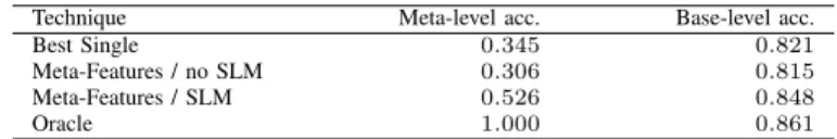
We will attempt to establish how useful the features ob-tained by Online Performance Estimation are. We do this by running the Meta-Feature Ensemble with various sets of features. One set contains only traditional features, (i.e., similar to [3]); the other both traditional meta-features and stream-based landmarkers. As the stream-based landmarkers are calculated using Online Performance Estima-tion, this shows the effect of Online Performance Estimation on the set of meta-features. Table III shows the results.

TABLE III. EFFECT OF STREAM-BASED LANDMARKERS.

Technique Meta-level acc. Base-level acc.

Best Single 0.345 0.821

Meta-Features / no SLM 0.306 0.815

Meta-Features / SLM 0.526 0.848

Oracle 1.000 0.861

The results show an increase in performance when stream-based landmarkers are used. Without stream-stream-based landmark-ers, theMeta-Feature Ensembleis outperformed by the

Best Single Classifier. When using stream-based landmarkers, both base-level and meta-level accuracy clearly increase. This supports the hypothesis that Online Performance Estimation is useful in the context of online classifier selection.

V. CONCLUSIONS

We have introduced the Online Performance Estimation framework, which can be used in data stream ensembles to weight the votes of ensemble members, in particular when using fundamentally different model types. We applied this approach to build a simple novel ensemble technique,BLAST, to evaluate its performance. Based on an extensive empirical evaluation we observe thatBLASTis statistically equivalent to current state of the art ensembles. It also outperforms the meta-learning attempts to combine various models, even though the underlying framework is significantly more elegant and does not require a database of earlier evaluations on data streams.

The experiments also suggest that Online Performance Estimation can be successfully leveraged to improve meta-learning approaches. Incorporating the obtained estimations in the Meta-Feature Ensemble clearly improves its performance. Moreover, our experiments show that the

Meta-Feature Ensemble relies highly on the novel meta-features derived from Online Performance Estimation.

Utilizing the Online Performance Estimation framework opens up a whole new line of data stream research. In this work we fixed the set of classifiers, whereas future work will explore which types of models and classifiers generally work well together. Rather than creating even more data stream classifiers, combining the current existing classifiers using Online Performance Estimation can elegantly lead to improved results. We believe that by exploring these possibilities we can further push the state of the art in data stream ensembles.

ACKNOWLEDGMENT

This work is supported by grant600.065.120.12N150from the Dutch Fund for Scientific Research (NWO).

REFERENCES

[1] J. Read, A. Bifet, B. Pfahringer, and G. Holmes, “Batch-incremental versus instance-incremental learning in dynamic and evolving data,” in

Advances in Intelligent Data Analysis XI. Springer, 2012, pp. 313–323. [2] D. H. Wolpert, “Stacked generalization,”Neural networks, vol. 5, no. 2,

pp. 241–259, 1992.

[3] J. N. van Rijn, G. Holmes, B. Pfahringer, and J. Vanschoren, “Algorithm Selection on Data Streams,” inDiscovery Science, ser. Lecture Notes in Computer Science. Springer, 2014, vol. 8777, pp. 325–336. [4] A. L. D. Rossi, A. C. P. de Leon Ferreira, C. Soares, and B. F. De Souza,

“MetaStream: A meta-learning based method for periodic algorithm selection in time-changing data,”Neurocomputing, vol. 127, pp. 52–64, 2014.

[5] N. C. Oza, “Online Bagging and Boosting,” in Systems, man and cybernetics, 2005 IEEE international conference on, vol. 3. IEEE, 2005, pp. 2340–2345.

[6] H. Wang, W. Fan, P. S. Yu, and J. Han, “Mining Concept-Drifting Data Streams using Ensemble Classifiers,” inKDD, 2003, pp. 226–235. [7] A. Bifet, G. Holmes, R. Kirkby, and B. Pfahringer, “MOA: Massive

Online Analysis,”Journal of Machine Learning Research, vol. 11, pp. 1601–1604, 2010.

[8] A. Bifet, G. Holmes, and B. Pfahringer, “Leveraging Bagging for Evolv-ing Data Streams,” inMachine Learning and Knowledge Discovery in Databases, ser. Lecture Notes in Computer Science. Springer, 2010, vol. 6321, pp. 135–150.

[9] J. Gama, R. Sebasti˜ao, and P. P. Rodrigues, “Issues in Evaluation of Stream Learning Algorithms,” inProceedings of the 15th ACM SIGKDD international conference on Knowledge discovery and data mining. ACM, 2009, pp. 329–338.

[10] J. Beringer and E. H¨ullermeier, “Efficient instance-based learning on data streams,”Intelligent Data Analysis, vol. 11, no. 6, pp. 627–650, 2007.

[11] L. Bottou, “Stochastic Learning,” in Advanced lectures on machine learning. Springer, 2004, pp. 146–168.

[12] S. Shalev-Shwartz, Y. Singer, N. Srebro, and A. Cotter, “Pegasos: primal estimated sub-gradient solver for SVM,”Mathematical Programming, vol. 127, no. 1, pp. 3–30, 2011.

[13] P. Domingos and G. Hulten, “Mining High-Speed Data Streams,” in

Proceedings of the sixth ACM SIGKDD international conference on Knowledge discovery and data mining, 2000, pp. 71–80.

[14] B. Pfahringer, G. Holmes, and R. Kirkby, “New Options for Hoeffding Trees,” inAI 2007: Advances in Artificial Intelligence. Springer, 2007, pp. 90–99.

[15] L. Breiman, “Bagging Predictors,”Machine learning, vol. 24, no. 2, pp. 123–140, 1996.

[16] R. E. Schapire, “The Strength of Weak Learnability,”Machine learning, vol. 5, no. 2, pp. 197–227, 1990.

[17] H.-L. Nguyen, Y.-K. Woon, W.-K. Ng, and L. Wan, “Heterogeneous En-semble for Feature Drifts in Data Streams,” inAdvances in Knowledge Discovery and Data Mining. Springer, 2012, pp. 1–12.

[18] J. Gama, P. Medas, G. Castillo, and P. Rodrigues, “Learning with Drift Detection,” inSBIA Brazilian Symposium on Artificial Intelligence, ser. Lecture Notes in Computer Science. Springer, 2004, vol. 3171, pp. 286–295.

[19] A. Bifet and R. Gavalda, “Learning from Time-Changing Data with Adaptive Windowing,” inSDM, vol. 7. SIAM, 2007, pp. 139–148. [20] J. Gama, P. Medas, and R. Rocha, “Forest Trees for On-line Data,”

in Proceedings of the 2004 ACM symposium on Applied computing. ACM, 2004, pp. 632–636.

[21] P. Brazdil, J. Gama, and B. Henery, “Characterizing the applicability of classification algorithms using meta-level learning,” in Machine Learning: ECML-94. Springer, 1994, pp. 83–102.

[22] J. Gama and P. Kosina, “Recurrent concepts in data streams classifica-tion,”Knowledge and Information Systems, vol. 40, no. 3, pp. 489–507, 2014.

[23] L. Breiman, “Random Forests,”Machine learning, vol. 45, no. 1, pp. 5–32, 2001.

[24] Q. Sun and B. Pfahringer, “Pairwise meta-rules for better meta-learning-based algorithm ranking,”Machine learning, vol. 93, no. 1, pp. 141– 161, 2013.

[25] A. Shaker and E. H¨ullermeier, “Recovery analysis for adaptive learning from non-stationary data streams: Experimental design and case study,”

Neurocomputing, vol. 150, pp. 250–264, 2015.

[26] J. Vanschoren, J. N. van Rijn, B. Bischl, and L. Torgo, “OpenML: networked science in machine learning,” ACM SIGKDD Explorations Newsletter, vol. 15, no. 2, pp. 49–60, 2014.

[27] M. Hall, E. Frank, G. Holmes, B. Pfahringer, P. Reutemann, and I. H. Witten, “The WEKA Data Mining Software: An Update,”ACM SIGKDD explorations newsletter, vol. 11, no. 1, pp. 10–18, 2009. [28] J. Demˇsar, “Statistical Comparisons of Classifiers over Multiple Data

Sets,” The Journal of Machine Learning Research, vol. 7, pp. 1–30, 2006.

View publication stats View publication stats