Bootstrap confidence sets under model misspecification

(1)

model misspecification

D i s s e rtat i o n

zur Erlangung des akademischen Grades

Dr. Rer. Nat.

im Fach Mathematik

eingereicht an der

Mathematisch-Naturwissenschaftlichen Fakult¨

at

Humboldt-Universit¨

at zu Berlin

von

Dipl.-Math. Mayya Zhilova

Pr¨

asident der Humboldt-Universit¨

at zu Berlin:

Prof. Dr. Jan-Hendrik Olbertz

Dekan der Mathematisch-Naturwissenschaftlichen Fakult¨

at:

Prof. Dr. Elmar Kulke

Gutachter:

1. Prof. Dr. Vladimir Spokoiny

2. Prof. Dr. Gilles Blanchard

3. Prof. Dr. Victor Chernozhukov

eingereicht am: 30. Juni 2015

(2)

(3)

(4)

(5)

The thesis studies a multiplier bootstrap procedure for construction of likelihood-based confidence sets in two cases. The first one focuses on a single parametric model, while the second case extends the construction to simultaneous confidence estimation for a collection of parametric models. Theoretical results justify the validity of the bootstrap procedure for a limited sample sizen, a large number of considered parametric models K, growing parameters’ dimensions, and possible misspecification of the parametric assumptions.

In the case of one parametric model the bootstrap approximation works if p3_/n _is

small, where p is the parameter’s dimension. The main result about bootstrap validity continues to apply even if the underlying parametric model is misspecified under the so-called Small Modelling Bias condition. If the true model deviates significantly from the considered parametric family, the bootstrap procedure is still applicable but it becomes a bit conservative: the size of the constructed confidence sets is increased by the modelling bias.

For the problem of construction of simultaneous confidence sets we suggest a multiplier bootstrap procedure for estimating the quantiles of the joint distribution of the likelihood ratio statistics, and for adjustment of the confidence level for multiplicity. Theoretical results state the bootstrap validity taking into account the bootstrap correction for multiplicity, they require the quantity (logK)12_p3

max/nto be small, wherepmaxis the maximal parameter

dimension. Here we also consider the situation when the parametric models are misspecified. If the models’ misspecification is significant, then the bootstrap critical values exceed the true ones and the simultaneous bootstrap confidence set becomes conservative.

The theoretical approach is based on several approximating bounds: non-asymptotic square-root Wilks theorem, Gaussian approximation of Euclidean norm of a sum of indepen-dent vectors, comparison and anti-concentration bounds for Euclidean norms of Gaussian vectors. Numerical experiments for misspecified linear, logistic, local constant and local quadratic regressions nicely confirm our theoretical results.

(6)

(7)

Diese Arbeit befasst sich mit einem Multiplier-Bootstrap Verfahren für die Konstruktion von Likelihood-basierten Konfidenzbereichen in zwei verschiedenen Fällen. Im ersten Fall betrachten wir das Verfahren für ein einzelnes parametrisches Modell und im zweiten Fall erweitern wir die Methode, um Konfidenzbereiche für eine ganze Familie von parametrischen Modellen simultan zu schätzen.

Theoretische Resultate zeigen die Validität der Bootstrap-Prozedur für eine potenziell begrenzte Anzahl an Beobachtungenn, eine große AnzahlK an betrachteten parametrischen Modellen, wachsende Parameterdimensionen und eine mögliche Misspezifizierung der parametrischen Annahmen. Im Falle eines einzelnen parametrischen Modells funktion-iert die Bootstrap-Approximation, wennp3_/n_{klein ist, wobei} _p_{hier die Parameterdimension}

bezeichnet. Das Hauptresultat über die Validität des Bootstrap gilt unter der sogenannten Small-Modelling-Bias Bedingung auch im Falle, dass das parametrische Modell misspezifiert ist. Wenn das wahre Modell signifikant von der betrachteten parametrischen Familie abweicht, ist das Bootstrap Verfahren weiterhin anwendbar, aber es führt zu etwas konservativeren Schätzungen: die Konfidenzbereiche werden durch den Modellfehler vergrößert.

Für die Konstruktion von simultanen Konfidenzbereichen entwickeln wir ein Multiplier-Bootstrap Verfahren um die Quantile der gemeinsamen Verteilung der Likelihood-Quotienten zu schätzen und eine Multiplizitätskorrektur der Konfidenzlevels vorzunehmen. Theoretische Ergebnisse zeigen die Validität des Verfahrens unter der Bedingung das (logK)12_p3

max/n

klein ist, wobei pmax die maximale Parameterdimension bezeichnet. Hier betrachten wir

auch wieder den Fall, dass die parametrischen Modelle misspezifiziert sind. Wenn die Misspezifikation signifikant ist, werden Bootstrap-generierten kritischen Werte gr¨oßer als die wahren Werte sein und die Bootstrap-Konfidenzmengen sind konservativ.

Die theoretische Untersuchung basiert auf einer Reihe von Approximationsresultaten: dem nicht-asymptotischen square-root Wilks Theorem, der Gaußschen Approximation der euklidischen Norm einer Summe von unabhängigen Vektoren, Vergleichsresultate und An-tikonzentrationsschranken für Normen von Gaußschen Vektoren. Numerische Experimente für misspezifizierte lineare, logistische, lokal konstante und lokal quadratische Regression bestätigen unsere theoretischen Ergebnisse.

(8)

(9)

First and foremost, I would like thank my supervisor Vladimir Spokoiny for his careful guidance and generous support during my PhD studies. I am very grateful to him for many inspiring and fruitful discussions, for his insightful comments and for being actively interested in my work during the whole period of my studies. I would also like to thank Prof. Reiß and Prof. H¨ardle for their important comments on my talks, which helped to improve this work.

I am very thankful to my friends and colleagues at the Weierstrass Institute for lots of helpful discussions, for their support and many cheerful moments. I am especially grateful to Andreas Andresen, Christian Bayer, Natalia Bochkina, Thorsten Dickhaus, Kirill Efimov, Roland Hildebrand, Marcel Ladkau, Nina Loginova, Hilmar Mai, Peter Math´e, Mario Maurelli, Tigran Nagapetyan, J¨org Polzehl, Konstantin Schildknecht, John Schoenmakers, Jens Stange, Karsten Tabelow, Niklas Willrich and Jianing Zhang.

An excellent working environment of the Weierstrass Institute helped me a lot to do this research, and I am cordially grateful to the institute’s directorate and administration for that. This research was supported by the German Research Foundation (DFG) through the Collaborative Research Center 649 “Economic Risk”.

(10)

(11)

Introduction

Bootstrap is a technique for making statistical inference about unknown population by resampling from an observed data set. The bootstrap was firstly introduced by Efron (1979), and since then became one of the most powerful and common tools in statistical confidence estimation and hypothesis testing. Bootstrap procedure is particularly useful for making inference in complicated statistical models, since it leads to a bootstrap world (see Efron and Tibshirani (1994), pp. 86-88), where all the objects are available for computation. Many versions and extensions of the original bootstrap method have been proposed in the literature; see e.g. Wu (1986); Mammen (1993); Newton and Raftery (1994); Janssen (1994); Barbe and Bertail (1995); Shao and Tu (1995); Horowitz (2001); Chatterjee and Bose (2005); Ma and Kosorok (2005); Chen and Pouzo (2009); Lavergne and Patilea (2013); B¨ucher and Dette (2013); Chen and Pouzo (2015) among many others.

This work focuses on the multiplier bootstrap procedure which attracted a lot of attention last time due to its nice theoretical properties and numerical performance. We mention the papers Chatterjee and Bose (2005), Arlot et al. (2010a,b) and Cher-nozhukov et al. (2013a, 2014a,b) for the most advanced recent results. Chatterjee and Bose (2005) showed some results on asymptotic bootstrap consistency in a very general framework: for estimators obtained by solving estimating equations. Arlot et al. (2010a) constructed a non-asymptotical confidence bound in `s-norm (s∈[1,∞]) for

the mean of a sample of high dimensional i.i.d. Gaussian vectors (or with a symmetric and bounded distribution), using generalized bootstrap for resampling of the quantiles. Arlot et al. (2010b) extended that results for the multiple testing problems for mean values of coordinates of high-dimensional i.i.d. Gaussian vectors with unknown co-variance matrix. They provided non-asymptotic control for the family-wise error rate using resampling-type procedures. Chernozhukov et al. (2013a) presented a number

(16)

2

of non-asymptotic results on Gaussian approximation and multiplier bootstrap for maxima of sums of high-dimensional vectors (with a dimension possibly much larger than a sample size) in a very general set-up. As one of the applications the authors considered the problem of multiple hypothesis testing in the framework of approximate means. They derived non-asymptotic results for the general stepdown procedure by Romano and Wolf (2005) with improved error rates and in high-dimensional setting. Chernozhukov et al. (2014a) showed how this technique applies to the problem of con-structing an honest confidence set in nonparametric density estimation. Chernozhukov et al. (2014b) extended the results from maxima to the class of sparsely convex sets. The present work makes a further step in studying the multiplier bootstrap method in the problems of confidence estimation and simultaneous confidence estimation by a quasi maximum likelihood method. For a rather general parametric model, we consider likelihood-based confidence sets (and simultaneous confidence sets) with the radius determined by a multiplier bootstrap. The aim of the study is to check the validity of the bootstrap procedure in the following setting:

1. the sample size n is fixed;

2. the parametric models can be misspecified;

3. the dimensions of the considered parametric models can be dependent on the sample size n;

4. in the case of simultaneous confidence estimation the number K of the para-metric models can be exponentially large w.r.t. n.

In the case of a single parametric model our results explicitly describe the error term of the bootstrap approximation. This particularly allows to track the impact of the parameter dimension p, the sample size n in the quality of the bootstrap procedure. As one of the corollaries, we show bootstrap validity under the constraint “p3/n-small”. Chatterjee and Bose (2005) stated results under the condition “p/n-small” but their results only apply to low dimensional projections of the MLE vector. In the likelihood based approach, the construction involves the Euclidean norm of the MLE, which leads to completely different tools and results. Chernozhukov et al. (2013a) allowed a huge parameter dimension with “ log(p)/n small” but they essentially work with a family of univariate tests which again differs essentially from the maximum likelihood approach.

Another interesting and important issue is the impact of the model misspecification on the accuracy of bootstrap approximation. A surprising corollary of our error bounds

(17)

is that the bootstrap confidence set can be used even if the underlying parametric model is slightly misspecified under the so-called small modelling bias (SmB) condition. If the modelling bias becomes large, the bootstrap confidence sets are still applicable, but they become more and more conservative. The (SmB) condition is given in Section 2.5 and it is consistent with classical bias-variance relation in nonparametric estimation. Numerical experiments in Section 2.4 nicely confirm our theoretical results. Below in this chapter we describe the problem and the theoretical approach in more detail, see Sections 1.1-1.3.

The problem of simultaneous confidence estimation appears in numerous practical applications when a confidence statement has to be made simultaneously for a collection of objects, e.g. in safety analysis in clinical trials, gene expression analysis, population biology, functional magnetic resonance imaging and many others. See e.g. Miller (1981); Westfall (1993); Manly (2006); Benjamini (2010); Dickhaus (2014), and references therein. This problem is also closely related to construction of simultaneous confidence bands in curve estimation, which goes back to Working and Hotelling (1929). For an extensive literature review about constructing the simultaneous confidence bands we refer to Hall and Horowitz (2013), Liu (2010), and Wasserman (2006).

A simultaneous confidence set requires a probability bound to be constructed jointly for several possibly dependent statistics. Therefore, the critical values of the corresponding statistics should be chosen in such a way that the joint probability distribution achieves a required family-wise confidence level. This choice can be made by multiplicity correction of the marginal confidence levels. The Bonferroni correction method (Bonferroni (1936)) uses a probability union bound, the corrected marginal significance levels are taken equal to the total level divided by the number of models. This procedure can be very conservative if the considered statistics are positively correlated and if their number is large. The ˇSid´ak correction method (ˇSid´ak (1967)) is more powerful than Bonferroni correction, however, it also becomes conservative in the case of large number of dependent statistics.

Most of the existing results about simultaneous bootstrap confidence sets and resampling-based multiple testing are asymptotic (with sample size tending to infinity), see e.g. Beran (1988, 1990); Hall and Pittelkow (1990); H¨ardle and Marron (1991); Shao and Tu (1995); Hall and Horowitz (2013), and Westfall (1993); Dickhaus (2014). The results based on asymptotic distribution of maximum of an approximating Gaussian process (see Bickel and Rosenblatt (1973); Johnston (1982); H¨ardle (1989)) require a huge sample size n, since they yield a coverage probability error of order (log(n))−1 (see Hall (1991)). Some papers considered an alternative approach in context of

(18)

4

confidence band estimation based on the approximation of the underlying empirical processes by its bootstrap counterpart. In particular, Hall (1993) showed that such an approach leads to a significant improvement of the error rate (see also Neumann and Polzehl (1998); Claeskens and Van Keilegom (2003)). Chernozhukov et al. (2014a) constructed honest confidence bands for nonparametric density estimators without requiring the existence of limit distribution of the supremum of the studentized empirical process: instead, they used an approximation between sup-norms of an empirical and Gaussian processes, and anti-concentration property of suprema of Gaussian processes.

In many modern applications the sample size cannot be large, and/or it can be smaller than a parameter dimension, for example, in genomics, brain imaging, spatial epidemiology and microarray data analysis, see Leek and Storey (2008); Kim and van de Wiel (2008); Arlot et al. (2010b); Cao and Kosorok (2011), and references therein. For the recent results on resampling-based simultaneous confidence sets in high-dimensional finite sample set-up we refer to the papers by Arlot et al. (2010b) and Chernozhukov et al. (2013a, 2014a,b), cited above in this section.

The present work’s set-up 1-4, in contrast with the paper by Chernozhukov et al. (2014b), does not require the sparsity condition, in particular the dimensions p1, . . . , pK

of each parametric family may grow with the sample size. Moreover, the simultane-ous likelihood-based confidence sets are not necessarily convex, and the parametric assumption can be violated.

The considered simultaneous multiplier bootstrap procedure involves two main steps: estimation of the quantile functions of the likelihood ratio statistics, and multiplicity correction of the marginal confidence level. Theoretical results state the bootstrap validity in the setting 1-4, taking in account the multiplicity correction. The resulting approximation bound requires the quantity (logK)12_p3

max/n to be small.

The log-factor here is suboptimal and can probably be improved. We particularly address the problem of the impact of the model misspecification. For the problem of simultaneous confidence estimation we introduce the “simultaneous small modelling bias condition” (SmB)d given in Section 3.4.2. This condition roughly means that

all the parametric models are close to the true distribution. If (SmB)d condition is

fulfilled, then the bootstrap approximation is accurate, otherwise the simultaneous bootstrap confidence set is still applicable, however, it becomes conservative. This property is nicely confirmed by the numerical experiments in Section 3.3.

Sections 1.1 - 1.3 below provide an introduction to the case of a single parametric model and give an overview of the theoretical approach. The problem of constructing

(19)

the simultaneous confidence sets is described in Section 1.4.

1.1 Likelihood-based confidence sets

The idea of constructing confidence intervals using the likelihood function goes back to Fisher (see Fisher (1956); Hudson (1971) and references therein). The Wilks phenomenon described below justifies this idea.

Let the data sample Y = (Y1, . . . , Yn)> consist ofindependent random observations

and belong to the probability space (Ω,F, IP) . We do not assume that the observations

Yi are identically distributed, moreover, no specific parametric structure of IP is

being required. In order to explain the idea of the approach we start here with a parametric case, however the assumption (1.1) below is not required for the results. Consider some known parametric family {IP(θ)} def= {IP(θ)µ0,θ∈Θ ⊂IRp}. If IP ∈ {IP(θ)}, then the true parameter θ∗ ∈Θ is such that

IP ≡IP(θ∗)∈ {IP(θ)}, (1.1)

and the initial problem of finding the properties of unknown distribution IP is reduced to the equivalent problem for the finite-dimensional parameter θ∗. The parametric family {IP(θ)} induces the log-likelihood process L(θ) of the sample Y :

L(θ) =L(Y,θ)def= log dIP(θ) dµ0 (Y)

and the maximum likelihood estimate (MLE) of θ∗:

e

θdef= argmax_θ∈ΘL(θ). (1.2)

The asymptotic Wilks phenomenon Wilks (1938) states that for the case of i.i.d. observations with the sample size tending to the infinity the likelihood ratio statistic converges in distribution to χ2_p/2 , where p is the parameter dimension:

2L(eθ)−L(θ∗) w

−→χ2_p, n→ ∞.

Define the likelihood-based confidence set as

E(z)def= nθ :L(θe)−L(θ)≤z2/2 o

,

then the Wilks phenomenon implies

IP n θ∗∈E(z_χ2 p(α)) o →α, n→ ∞,

(20)

6 1.2. Multiplier bootstrap procedure for the case of one parametric model

where z2_χ2

p(α) is the (1−α) -quantile for the χ

2

p distribution. This result is very

important and useful under the parametric assumption, i.e. when (1.1) holds. In this case the limit distribution of the likelihood ratio is independent of the model parameters or in other words it ispivotal. By this result a sufficiently large sample size allows to construct the confidence sets for θ∗ with a given coverage probability. However, a possibly low speed of convergence of the likelihood ratio statistic makes the asymptotic Wilks result hardly applicable to the case of small or moderate samples. Moreover, the asymptotical pivotality breaks down if the parametric assumption (1.1) does not hold (see Huber (1967); White (1982)) and, therefore, the whole approach may be misleading if the model is considerably misspecified. If the assumption (1.1) does not hold, then the “true” parameter is defined by the projection of the true measure IP on the parametric family {IP(θ)}:

θ∗def= argmax θ∈Θ IEL(θ), (1.3) or equivalently θ∗def= argmin θ∈Θ KL (IP, IP(θ)).

The recent results by Spokoiny (2012a, 2013) provide a non-asymptotic version of square-root Wilks phenomenon for the case of misspecified model. It holds with an exponentially high probability

q 2 L(θe)−L(θ∗) − kξk ≤∆W' p √ n, (1.4) where ξ def= D₀−1∇θL(θ∗) , D02 def = −∇2 θIEL(θ ∗

) . The bound is non-asymptotical, the approximation error term ∆W has an explicit form (the precise statement is given in

Theorem A.2, Section A.1), and it depends on the parameter dimension p, sample size n, and the probability of the random set on which the result holds.

Due to this bound, the original problem of finding a quantile of the LR test statistic

L(eθ)−L(θ∗) is reduced to a similar question for the approximating quantity kξk.

The difficulty here is that in general kξk is non-pivotal, it depends on the unknown distribution IP and the target parameter θ∗.

1.2 Multiplier bootstrap procedure for the case of one

parametric model

In the present work we study themultiplier bootstrap (orweighted bootstrap) procedure for estimation of the quantiles of the likelihood ratio statistic. The idea of the procedure

(21)

is to mimic a distribution of the likelihood ratio statistic by reweighing its summands with random multipliers independent of the data:

Lab(θ)def= Xn i=1log dIPθ dµ0 (Yi) ui.

Here the probability distribution is taken conditionally on the data Y , which is denoted by the sign ab (also IEab and Varab denote expectation and variance operators w.r.t. the probability measure conditional on Y ). The random weights u1, . . . , un

are i.i.d., independent of Y and it holds for them: IEab(ui) = 1 , Varab(ui) = 1 ,

IEabexp(ui)<∞. Therefore, the multiplier bootstrap induces the probability space

conditional on the data Y . A simple but important observation is that IEabLab(θ)≡ L(θ) , and hence,

argmax_θIEabLab(θ) = argmax_θL(θ) =eθ. (1.5)

This means that the target parameter in the bootstrap world is precisely known and it coincides with the maximum likelihood estimator eθ conditioned on Y , therefore, the

bootstrap likelihood ratio statistic Lab(eθ

ab )−Lab(eθ) def = sup_θ∈ΘL ab (θ)−Lab(θe) is fully

computable and leads to a simple computational procedure for the approximation of the distribution of L(eθ)−L(θ∗) .

1.3 Theoretical justification of the bootstrap for the case

of one parametric model

The goal of the present study is to show the validity of the described multiplier bootstrap procedure in a fixed sample size set-up, and to obtain an explicit bound on the error of coverage probability. In other words, we are interested in non-asymptotic approximation of the distribution of

L(θe) −L(θ∗)

1/2

with the distribution of

Lab(θe

ab

)−Lab(eθ) 1/2

. So far there exist very few theoretical non-asymptotic results about bootstrap validity. Classical asymptotic tools for showing the bootstrap con-sistency are based on weak convergence arguments which are not applicable in the finite sample set-up. Some different methods have to be applied. In particular, the approach of Liu (1988) based on Berry-Esseen theorem can be extended to a finite sample set-up with a univariate parameter. For a high dimensional parameter space, important contributions are done in the recent papers by Arlot et al. (2010a) and Chernozhukov et al. (2013a, 2014b). The latter papers used a Gaussian approximation, Gaussian comparison, and Gaussian anti-concentration technique in high dimension. Our approach is similar but we combine it with the square-root Wilks expansion and

(22)

81.3. Theoretical justification of the bootstrap for the case of one parametric model

use Pinsker’s inequality for Gaussian comparison and anti-concentration steps. The main steps of our theoretical study are illustrated by the following scheme:

sq-Wilks theorem Gauss. approx. Y-world: q 2L(eθ)−2L(θ∗) ≈ p/√n kξk ≈w (p3_/n₎1/8 kξk w _≈ √pδ2 smb _compar.Gauss. (1.6) Bootstrap world: q 2Lab(eθ ab )−2Lab(θe) ≈ p/√n kξabk ≈w (p3_/n₎1/8 kξabk where ξab def= ξab(θ∗)def= D₀−1∇_θ[Lab(θ∗)−IEabLab(θ∗)]. (1.7) The vectors ξ and ξab are zero mean Gaussian and they mimic the covariance structure of the vectors ξ and ξab: ξ∼N(0,Varξ) , ξab∼N 0,Varabξab

.

The error term shown below each arrow corresponds to the i.i.d. case considered in details in Section A.3.1. The upper line of the scheme corresponds to the Y -world, the lower line - to the bootstrap world. In both lines we apply two steps for approximating the corresponding likelihood ratio statistics. The first approximating step is the non-asymptotic square-root Wilks theorem: the bound (1.4) for the Y -case and a similar statement for the bootstrap world, which is obtained in Theorem A.4, Section A.2. The corresponding error is of order p/√n for the case of i.i.d. observations; in the bootstrap world the square-root Wilks expansion implies

q 2Lab(θe ab )−2Lab(eθ)− kξ ab (eθ)k ≤Cp/√n (1.8) for ξab(θ) def= D₀−1∇_θ

Lab(θ) −IEabLab(θ). In our approximation diagram we use ξab(θ∗) instead of ξab(eθ) which is more convenient for the GAR step and is justified

by Lemma A.2 showing that ξ

ab (θe)−ξ ab (θ∗)≤Cp/ √ n.

The next step is called Gaussian approximation (GAR) which means that the distribution of the Euclidean norm kξk of a centered random vector ξ is close to the distribution of the similar norm of a Gaussian vector kξk with the same covariance matrix as ξ. A similar statement holds for the vector ξab. Thus, the initial problem of comparing the distributions of the likelihood ratio statistics is reduced to the comparison of the distributions of the Euclidean norms of two centered normal vectors ξ and ξab (Gaussian comparison). This last step links their distributions and encloses the approximating scheme. The Gaussian comparison step is done by computing the Kullback-Leibler divergence between two multivariate Gaussian distributions (i.e.

(23)

by comparison of the covariance matrices of ∇θL(θ∗) and ∇θLab(θ∗) ) and applying

Pinsker’s inequality (Lemma B.5. At this point we need to introduce the “small modelling bias” condition (SmB) from Section 3.4.2. It is formulated in terms of the following nonnegative-definite p×p symmetric matrices:

H₀2 def= Xn i=1IE h ∇_θì(θ∗)∇θì(θ∗)> i , (1.9) B₀2 def= Xn i=1IE[∇θì(θ ∗_)]_IE_[_∇ θì(θ∗)]> (1.10) for ì(θ) def = log dIPθ dµ0(Yi)

, so that Var{∇θL(θ∗)} = H₀2 −B₀2. If the parametric assumption (1.1) is true or if the data Y are i.i.d., then it holds IE[∇_θ`i(θ∗)]≡0

and B2

0 = 0 . The (SmB) condition roughly means that the bias term B02 is small

relative to H₀2. Below we show that the Kullback-Leibler distance between the distributions of two Gaussian vectors ξ and ξab is bounded by pkH₀−1B2₀H₀−1k2_/_{2 .}

The (SmB) condition precisely means that this quantity is small (in scheme (1.6) it is denoted by √pδ2_smb). In Section A.3.4 the value kH₀−1B₀2H₀−1k is evaluated for some commonly used models: the case of i.i.d. observations, generalized linear model and linear quantile regression. Below we distinguish between two situations: when the condition (SmB) is fulfilled and the opposite case. Theorems 2.1 and 2.2 in Section 2.1 deal with the first case, it provide the cumulative error term for the coverage probability of the confidence set (1.1), taken at the (1−α) -quantile computed with the multiplier bootstrap procedure. The proof of this result (see Section D.1.1) summarizes the steps of scheme (1.6). The biggest term in the full error is induced by Gaussian approximation and requires the ratio p3/n to be small. In the case of a “large modelling bias”, i.e. when (SmB) does not hold, the multiplier bootstrap procedure continues to apply. It turns out that the bootstrap quantiles increase with the growing modelling bias, hence, the confidence set based on it remains valid, however, it may become conservative. This result is given in Theorem 2.4 of Section 2.1. The problems of Gaussian approximation and comparison for the Euclidean norm are considered in Sections C.1 and B.4 in general terms independently of the statistical setting of the thesis, and might be interesting by themselves. Section B.4 presents also an anti-concentration inequality for the Euclidean norm of a Gaussian vector. This inequality shows how the deviation probability changes with a threshold. The general results on GAR are summarized in Theorem B.1 and restated in Proposition D.1 for the setting of scheme (1.6). These results are also non-asymptotic with explicit errors and apply under the condition that the ratio p3/n is small.

In Theorem 2.3 we consider the case of a scalar parameter p= 1 with an improved error term. Furthermore in Section 2.3 we propose a modified version of a quantile

(24)

10 1.4. Simultaneous confidence sets

function based on a smoothed probability distribution. In this case the obtained error term is also better than in the general result.

1.4 Simultaneous confidence sets

Here we use the notations from Section 1.1. Let the random data

Y def= (Y1, . . . , Yn)> (1.11)

consist ofindependent observations Yi, and belong to the probability space (Ω,F, IP) .

The sample size n isfixed. IP is an unknown probability distribution of the sample Y . Consider K parametric families of probability distributions:

{IPk(θ)} def

= {IPk(θ)µ0,θ∈Θk⊂IRpk}, k= 1, . . . , K.

Each parametric family induces the quasi log-likelihood function for θ∈Θk⊂IRpk

Lk(Y,θ) def = log dIPk(θ) dµ0 (Y) =Xn i=1log dIPk(θ) dµ0 (Yi) . (1.12)

It is important that wedo not require that IP belongs to any of the known parametric families {IPk(θ)}, that is why the term quasi log-likelihood is used here. Below in

this section we consider two popular examples of simultaneous confidence sets in terms of the quasi log-likelihood functions (1.12). Namely, the simultaneous confidence band for local constant regression, and multiple quantiles regression.

The target of estimation for the misspecified log-likelihood Lk(θ) is such a

pa-rameter θ∗_k, that minimises the Kullback-Leibler distance between the unknown true measure IP and the parametric family {IPk(θ)}:

θ∗_k def= argmax

θ∈Θk

IELk(θ). (1.13)

The maximum likelihood estimator is defined as:

e θk def = argmax θ∈Θk Lk(θ).

The parametric sets Θk have dimensions pk, therefore, θe_k,θ∗_k∈IRpk. For 1≤k, j ≤ K and k6=j the numbers pk and pj can be unequal.

The likelihood-based confidence set for the target parameter θ∗_k is

Ek(z) def = n θ∈Θk:Lk(θe_k)−L_k(θ)≤z2/2 o ⊂IRpk_. _(1.14)

(25)

Let zk(α) denote the (1−α) -quantile of the corresponding square-root likelihood ratio statistic: z_k(α)def= inf n z≥0 :IP Lk(eθ_k)−L_k(θ∗_k)>z2/2 ≤α o . (1.15)

Together with (1.14) this implies for each k= 1, . . . , K:

IP

θ∗_k∈Ek(zk(α))

≥1−α. (1.16)

Thus Ek(z) and the quantile function zk(α) fully determine the marginal (1−α)

-confidence set. The simultaneous -confidence set requires a correction for multiplicity. Let c(α) denote a maximal number c∈(0, α] s.t.

IP [K k=1 nq 2Lk(eθ_k)−2L_k(θ∗_k)>z_k(c) o ≤α. (1.17) This is equivalent to c(α)def= sup ( c∈(0, α] :IP max 1≤k≤K q 2Lk(eθ_k)−2L_k(θ∗_k)−z_k(c) >0 ≤α ) . (1.18) Therefore, taking the marginal confidence sets with the same confidence levels 1−c(α) yields the simultaneous confidence bound of the total level 1−α. The value c(α)∈ (0, α] is the correction for multiplicity. In order to construct the simultaneous confidence set using this correction, one has to estimate the values z_k(c(α)) for all k= 1, . . . , K. By definition this problem splits into two subproblems:

1. Marginal step. Estimation of the marginal quantile functions z1(α) , . . . , z_K(α) given in (1.15).

2. Correction for multiplicity. Estimation of the correction for multiplicity

c(α) given in (1.18).

If the 1 -st problem is solved for any α ∈(0,1) , the 2 -nd problem can be treated by calibrating the value α s.t. (1.18) holds. It is important to take into account the correlation between the likelihood ratio statistics Lk(eθ_k)−L_k(θ∗_k) , k = 1, . . . , K,

otherwise the estimate of the correction c(α) can be too conservative. For instance, the Bonferroni correction would lead to the marginal confidence level 1−α/K, which may be very conservative if K is large and the statistics Lk(eθ_k)−L_k(θ∗_k) are highly

correlated.

In Section 3.1 we suggest a multiplier bootstrap procedure, which performs the steps 1 and 2 described above. Theoretical justification of the procedure is given in Section

(26)

12 1.4. Simultaneous confidence sets

3.2. The proofs are based on several approximation bounds: non-asymptotic square-root Wilks theorem, simultaneous Gaussian approximation for `2-norms, Gaussian

comparison, and simultaneous Gaussian anti-concentration inequality.

In the Sections 1.1, 1.2 above we introduced the 1 -st subproblem: it is considered only one parametric model (K = 1 ) there. Chapter 2 studies a multiplier procedure in detail for this case. Chapter 3 extends the construction to simultaneous confidence estimation for a collection of parametric models, however, the results about simultane-ous confidence sets do not follow directly from the 1-model case, and require the use different technical tools.

Below we illustrate the definitions (1.12)-(1.18) of the simultaneous likelihood-based confidence sets with two popular examples.

Example 1 (Simultaneous confidence band for local constant regression):

Let Y1, . . . , Yn be independent random scalar observations and X1, . . . , Xn some

deterministic design points. Consider the following quadratic likelihood function reweighted with the kernel functions K(·) :

L(θ, x, h)def= −1 2 Xn i=1(Yi−θ) 2_w i(x, h), wi(x, h)def= K({x−Xi}/h), K(x)∈[0,1], Z IR K(x)dx= 1, K(x) =K(−x).

Here h >0 denotes bandwidth, the local smoothing parameter. The target point and

the local MLE read as: θ∗(x, h)def= Pn i=1wi(x, h)IEYi Pn i=1wi(x, h) , θe(x, h) def = Pn i=1wi(x, h)Yi Pn i=1wi(x, h) . e

θ(x, h) is also known as Nadaraya-Watson estimate. Fix a bandwidth h and consider the range of points x1, . . . , xK. They yield K local constant models with the target

parameters θ∗_k def= θ∗(xk, h) and the likelihood functions Lk(θ) def

= L(θ, xk, h) for

k= 1, . . . , K. The confidence intervals for each model are defined as

Ek(z, h) def

= nθ∈Θ:L(eθ(x_k, h), x_k, h)−L(θ, x_k, h)≤z2/2 o

,

with the quintile functions z_k(α) and for the multiplicity correction c(α) from (1.15) and (1.18) they form the following simultaneous confidence band:

IP \K k=1 n θ∗_k∈Ek zk(c(α)) o ≥1−α.

(27)

Example 2 (Multiple quantiles regression): Quantile regression is an impor-tant method of statistical analysis, widely used in various applications. It aims at estimating conditional quantile functions of a response variable, see Koenker (2005). Multiple quantiles regression model considers simultaneously several quantile regres-sion functions based on a range of quantile indices, see e.g. Liu and Wu (2011); Qu (2008); He (1997). Let Y1, . . . , Yn be independent random scalar observations and

X1, . . . , Xn ∈IRd some deterministic design points, as in Example 1. Consider the

following quantile regression models for k= 1, . . . , K:

Yi=gk(Xi) +εk,i, i= 1, . . . , n,

where gk(x) :IRd7→IR are unknown functions, the random values εk,1, . . . , εk,n are

independent for each fixed k, and

IP(εk,i<0) =τk for all i= 1, . . . , n.

The range of quantile indices τ1, . . . , τK ∈(0,1) is known and fixed. We are interested

in simultaneous parametric confidence sets for the functions g1(·), . . . , gK(·) . Let

fk(x,θ) :IRd×IRpk 7→IR be known regression functions. Using the quantile regression

approach by Koenker and Bassett Jr (1978), this problem can be treated with the quasi maximum likelihood method and the following log-likelihood functions:

Lk(θ) =− Xn i=1ρτk(Yi−fk(Xi,θ)), ρτk(x) def = x(τk−1I{x <0}).

for k= 1, . . . , K. This quasi log-likelihood function corresponds to the Asymmetric

Laplace distribution with the density function τk(1−τk)e−ρτk(x−a). If τ = 1/2 , then

ρ₁_/₂(x) = |x|/2 and L(θ) = −Pn

i=1|Yi−fk(Xi,θ)|/2 , which corresponds to the

median regression.

1.5 Notation

k · k is the Euclidean norm for vectors and spectral norm for matrices;

k · kmax is the maximum of absolute values of elements of a vector or of a matrix;

k · k₁ is the sum of absolute values of elements of a vector or of a matrix.

1K def

= (1, . . . ,1)>∈IRK,

psum

def

= p1+· · ·+pK, pmaxdef= max 1≤k≤Kpk.

(28)

14 1.6. Organization of the thesis

C is a generic constant. The value x>0 describes our tolerance level: all the results will be valid on a random set of probability ( 1−Ce−x_{) for an explicit constant} _C_.

Everywhere we show how the error bounds depend on p, p1, . . . , pK and n for the

case of the i.i.d. observations Y1, . . . , Yn and x≤Clogn. More details on it are given

in Section A.3.1. In Section A.3 we also consider generalised linear model and linear quantile regression, and show for them the dependence on p, p1, . . . , pK and n of all

the values appearing in main results and their conditions.

1.6 Organization of the thesis

• Chapter 2 considers the case of one parametric model, it includes:

– Section 2.1 with description of the multiplier bootstrap procedure,

– Sections 2.2, 2.3 with theoretical results justifying the procedure and Section 2.5 with the required conditions, in Section 2.5.3 we check the (SmB)

condition for some popular models,

– Section 2.4 with the results of numerical experiments for simulated data. We check the performance of the bootstrap procedure for small sample sizes ( 50 and 100 ) in the following cases:

i. linear regression model

a) without any misspecification,

b) with misspecified heteroscedastic noise,

c) with misspecified both regression function and noise, and with growing modelling bias,

ii. logistic regression with growing modelling bias;

• Chapter 3 studies the problem of simultaneous confidence estimation, it includes:

– Section 3.1 with description of the simultaneous multiplier bootstrap proce-dure,

– Sections 3.2.1 and 3.2.2 with an overview of the theoretical approach and the theoretical results showing the bootstrap validity. The imposed conditions are given in Section 3.4,

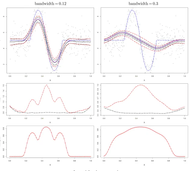
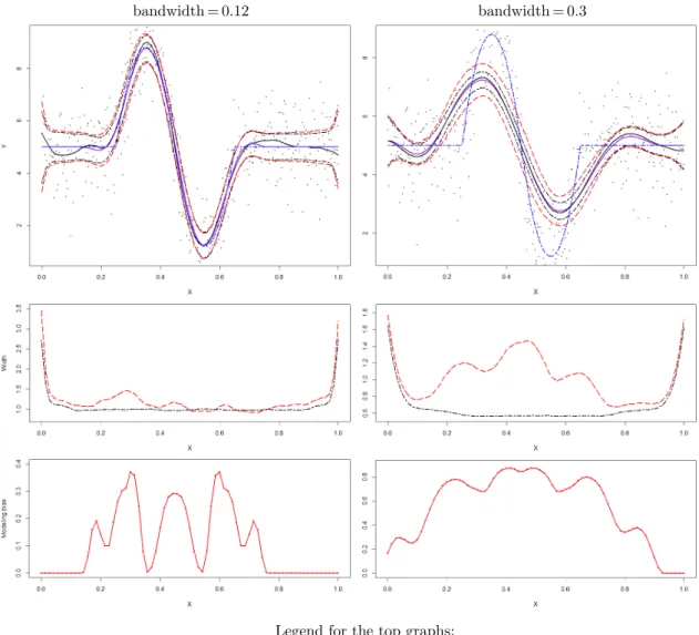
– Section 3.3 describing the results of numerical experiments. We construct simultaneous confidence corridors for local constant and local quadratic regressions using both bootstrap and Monte Carlo procedures. The quality

(29)

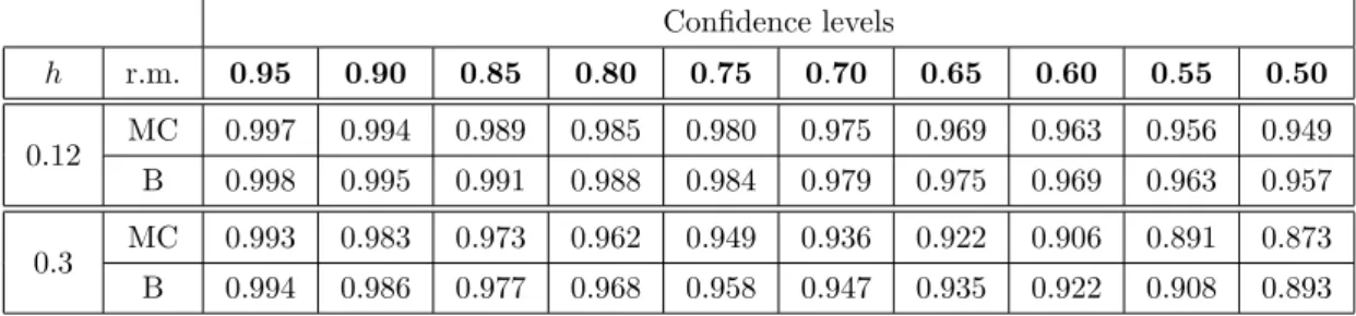
of the bootstrap procedure is checked by computing the effective simul-taneous coverage probabilities of the bootstrap confidence sets. We also compare the widths of the confidence bands and the values of multiplic-ity correction obtained with bootstrap and with Monte Carlo procedures. The experiments confirm that the simultaneous bootstrap confidence sets and the bootstrap multiplicity correction become conservative if the local parametric model is considerably misspecified;

• The Appendix consists of Chapters A-D:

– Chapter A collects the statements about non-asymptotic square-root Wilks approximations for Y and bootstrap worlds. In Section A.3 these results are specified for some common models: i.i.d. observations, generalised linear model and linear median regression, we also show the dependence of the non-asymptotic bounds on sample size and parameter’s dimension.

– Chapter B presents some useful statements about approximations between distributions of `2-norms of sums of independent random vectors. Namely,

Gaussian approximation, Gaussian comparison and anti-concentration in-equality.

– Chapter C provides similar results as in Chapter B for joint distributions of sets of `2-norms of sums of independent random vectors.

– Chapter D contains proofs of the main results.

The results presented in Chapters 2 and 3 are based on the papers Spokoiny and Zhilova (2015) and Zhilova (2015) respectively.

(30)

(31)

Bootstrap likelihood-based

confidence sets

A multiplier bootstrap procedure for construction of likelihood-based confidence sets is considered for finite samples and a possible model misspecification. Theoretical results justify the bootstrap validity for a small or moderate sample size and allow to control the impact of the parameter dimension p: the bootstrap approximation works if p3_/n _{is small. The main result about bootstrap validity}

continues to apply even if the underlying parametric model is misspecified under the so-called small modelling bias condition. In the case when the true model deviates significantly from the considered parametric family, the bootstrap procedure is still applicable but it becomes a bit conservative: the size of the constructed confidence sets is increased by the modelling bias. We illustrate the results with numerical examples for misspecified linear and logistic regression models.

2.1 Multiplier bootstrap procedure

Let `i(θ) denote the parametric log-density of the i-th observation:

`i(θ) def = log dIPθ dµ0 (Yi) , then L(θ) =Pn

i=1`i(θ). Consider i.i.d. scalar random variables ui independent of

Y with IEui = 1 , Varui = 1 , IEexp(ui) < ∞ for all i = 1, . . . , n. Multiply the

summands of the likelihood function L(θ) with the new random variables:

Lab(θ)def= Xn

i=1`i(θ)ui,

(32)

18 2.2. Main results

then it holds IEabLab(θ) = L(θ) , where IEab stands for the conditional expectation given Y . Therefore, the quasi MLE for the Y -world is a target parameter for the bootstrap world:

argmax_θ_∈_ΘIEabLab(θ) = argmax_θ_∈_ΘL(θ) =eθ.

The corresponding quasi MLE under the conditional measure IPab is defined as

e

θabdef= argmax_θ∈ΘL

ab (θ).

The likelihood ratio statistic in the bootstrap world is equal to Lab(eθ

ab

)−Lab(eθ) in

which all the entries are known including the function Lab(θ) and the arguments eθ

ab ,

e

θ.

Let 1−α∈(0,1) be a known desirable confidence level of the set E(z) :

IP(θ∗ ∈E(z))≥1−α. (2.1)

Here the parameter z≥0 determines the size of the confidence set. Define z(α) as the minimal possible value of z such that (2.1) is fulfilled:

z(α)def= infnz≥0 :IPL(eθ)−L(θ∗)>z2/2

≤αo. (2.2)

For evaluating this value we apply the multiplier bootstrap procedure which replaces the unknown data distribution with the artificial bootstrap distribution given the observed sample. The target value z(α) is approximated by the value zab(α) defined as the upper α-quantile of 2Lab(eθ

ab )−2Lab(eθ) 1/2 : zab(α)def= inf n z≥0 :IP ab Lab(eθ ab )−Lab(eθ)>z2/2 ≤α o . (2.3)

Note that the bootstrap probability IP ab and log-likelihood excess Lab(eθ

ab

)−Lab(eθ)

depends on the data Y and thus, zab(α) is random as well. Theoretical results of the next section justify the proposed approach.

2.2 Main results

Now we state the main results for the general set-up. The approximating error terms and the conditions are specified in Section A.3 for popular examples including i.i.d. observations, generalised regression model and linear quantile regression. Our first result claims that the random quantity IPabLab(eθ

ab

)−Lab(eθ) > z2/2

is close in probability to the value IPL(θe)−L(θ∗)>z2/2

(33)

Theorem 2.1. Let the conditions of Section 2.5 be fulfilled, then it holds for z ≥ max{2,√p}+C(p+x)/√n with probability ≥1−12e−x_:

IP L(eθ)−L(θ∗)>z2/2 −IPabLab(eθ ab )−Lab(eθ)>z2/2 ≤∆full.

The error term ∆full≤C{(p+x)3/n}1/8 in the case of i.i.d. model; see Section A.3.1.

Explicit definition of the error term ∆full is given in Section D.1.1, see (D.9) and

(D.11) therein.

The term ∆full can be viewed as a sum of the error terms corresponding to each

step in the scheme (1.6). The largest error term equal to C{(p+x)3/n}1/8 _{is induced}

by GAR. This error rate is not always optimal for GAR, e.g. in the case of p= 1 or for the i.i.d. observations (see Remark B.2). In Theorems 2.3 and 2.5 the rate is C{(p+x)3/n}1/2_.

The next result can be viewed as “bootstrap validity”.

Theorem 2.2 (Validity of the bootstrap under a small modelling bias). Assume the conditions of Theorem 2.1. Then for α≤1−8e−x_{, it holds}

IP L(eθ)−L(θ∗)>(z ab (α))2/2 −α ≤∆z,full. (2.4)

The error term ∆z,full≤C{(p+x)3/n}1/8 in the case of i.i.d. model; see Section A.3.1.

For a precise description see (D.17) and (D.18).

In view of definition (1.1) of the likelihood-based confidence set Theorem 2.1 implies the following

Corollary 2.1 (Coverage probability error). Under the conditions of Theorem 2.2 it holds:

|IP{θ∗∈E(zab(α))} −(1−α)| ≤∆z,full.

Remark 2.1 (Critical dimension). The error term ∆full depends on the ratio p3/n.

The bootstrap validity can be only stated if this ratio is small. The obtained error bound seems to be mainly of theoretical interest, because the condition “ (p3/n)1/8 is small” may require a huge sample. However, it provides some qualitative information about the bootstrap behavior as the parameter dimension grows. Our numerical results show that the accuracy of bootstrap approximation is very reasonable in a variety of examples with pn.

In the following theorem we consider the case of the scalar parameter p= 1 . The obtained error rate is 1/√n, which is sharper than 1/n1/8. Instead of the GAR for the Euclidean norm from Section B we use here Berry-Esseen theorem (see also Remark B.2).

(34)

20 2.2. Main results

Theorem 2.3 (The case of p= 1 , using Berry-Esseen theorem). Let the conditions of Section 2.5 be fulfilled.

1. For z≥1 +C(1 +x)/√n, it holds with probability ≥1−12e−x IP L(θe)−L(θ∗)>z2/2 −IPab Lab(eθ ab )−Lab(eθ)>z2/2 ≤∆B.E.,full; (2.5) 2. For α≤1−8e−x IP L(eθ)−L(θ∗)>(z ab (α))2/2 −α ≤∆B.E.z,full. (2.6)

The error terms ∆B.E.,full, ∆B.E.z,full≤C(1 +x)/

√

n in the case A.3.1. Explicit defini-tions of ∆B.E.,full is given in (D.20) and (D.21) in Section D.1.1.

Remark 2.2(Bootstrap validity and weak convergence). The standard way of proving the bootstrap validity is based on weak convergence arguments; see e.g. Mammen (1992), van der Vaart and Wellner (1996), Janssen and Pauls (2003), Chatterjee and Bose (2005). If the statistic L(eθ)−L(θ∗) weakly converges to a χ2-type distribution,

one can state an asymptotic version of the results of Theorems 2.1, 2.3. Our way is based on a kind of non-asymptotic Gaussian approximation and Gaussian comparison for random vectors and allows to get explicit error terms.

Remark 2.3(Use of Edgeworth expansion). The classical results on confidence sets for the mean of population states the accuracy of order 1/n based on the second order Edgeworth expansion, see Hall (1992). Unfortunately, if the considered parametric model can be misspecified, even the leading term is affected by the modelling bias, and the use of Edgeworth expansion cannot help in improving the bootstrap accuracy.

Remark 2.4 (Choice of the weights). In our construction, similarly to Chatterjee and Bose (2005), we apply a general distribution of the bootstrap weights ui under

some moment conditions. One particularly can use Gaussian multipliers as suggested by Chernozhukov et al. (2013a). This leads to the exact Gaussian distribution of the vectors ξab and is helpful to avoid one step of Gaussian approximation for these vectors.

Remark 2.5 (Skipping the Gaussian approximation step). The biggest error term C{(p+x)3/n}1/8 _{in Theorem 2.1 is induced by the Gaussian approximation step. In}

some particular cases the Gaussian approximation step can be avoided leading to better error bounds. For example, if the marginal score vectors ∇θ`i(θ∗) are normally

distributed, and the random bootstrap weights are normal as well, ui ∼N(1,1) , then

(35)

If the marginal score vectors ∇θ`i(θ∗) are i.i.d. and symmetrically distributed (s.t.

∇_θ`i(θ∗)∼ −∇θ`i(θ∗) ), and the centered bootstrap weights follow the Rademacher

distribution (ui ∼2Bernoulli(0.5) ), then the recent results by Arlot et al. (2010a) can

be applied to show that the conditional distribution of kξab(θ∗)k given the data is close to the distribution of kξk. However, such methods require some special structural conditions on the underlying measure IP like symmetricity or Gaussianity of the errors and may fail if these conditions are violated. It remains a challenging question how a nice performance of a general bootstrap procedure even for small or moderate samples can be explained.

Now we discuss the impact of modelling bias, which comes from a possible misspeci-fication of the parametric model. As explained by the approximating diagram (1.6), the distance between the distributions of the likelihood ratio statistics can be characterized via the distance between two multivariate normal distributions. To state the result let us recall the definition of the full Fisher information matrix D2₀ def= −∇2

θIEL(θ

∗_{) .} For the matrices H2

0 and B02, given in (1.9) and (1.10), it holds H02 > B02 ≥0 . If

the parametric assumption (1.1) is true or in the case of an i.i.d. sample Y , B₀2= 0 . Under the condition (SmB) kH₀−1B₀2H₀−1k enters linearly in the error term ∆full in

Theorem 2.1.

The first statement in Theorem 2.4 below says that the effective coverage probability of the confidence set based on the multiplier bootstrap is larger than the nominal coverage probability up to the error term ∆b,full ≤C{(p+x)3/n}1/8. The inequalities

in the second part of Theorem 2.4 prove theconservativeness of the bootstrap quantiles: the quantity q tr{D−₀1H2 0D −1 0 } − q tr{D₀−1(H2 0 −B02)D −1

0 } ≥0 increases with the

growing modelling bias.

Theorem 2.4 (Performance of the bootstrap for a large modelling bias). Under the conditions of Section 2.5 except for (SmB) it holds for z≥max{2,√p}+C(p+x)/√n

with probability ≥1−14e−x

1. IP L(eθ)−L(θ∗)>z2/2 ≤IPab Lab(eθ ab )−Lab(eθ)>z2/2 +∆b,full. 2. zab(α)≥z(α+∆b,full) + q tr{D−₀1H₀2D₀−1} − q tr{D−₀1(H₀2−B₀2)D−₀1} −∆qf,1, zab(α)≤z(α−∆b,full) + q tr{D−₀1H2 0D −1 0 } − q tr{D−₀1(H2 0 −B02)D −1 0 }+∆qf,2.

(36)

22 2.3. Smoothed version of a quantile function

The term ∆b,full≤C{(p+x)3/n}1/8 is given in (D.23) in Section D.1.2. The positive

values ∆qf,1, ∆qf,2 are given in (D.28),(D.27)in Section D.1.2, they are bounded from

above with (a2+a2_B)(√8xp+ 6x) for the constants a2 >0,a2_B ≥0 from conditions

(I), (IB).

Remark 2.6. There exists some literature on robust (and heteroscedasticity robust) bootstrap procedures; see e.g. Mammen (1993), Aerts and Claeskens (2001), Kline and Santos (2012). However, up to our knowledge there are no robust bootstrap procedures for the likelihood ratio statistic, most of the results compare the distribution of the estimator obtained from estimating equations, or Wald / score test statistics with their bootstrap counterparts in the i.i.d. setup. In our context this would correspond to the noise misspecification in the log-likelihood function and it is addressed automatically by the multiplier bootstrap. Our notion of modelling bias includes the situation when the target value θ∗ from (1.3) only defines a projection (the best parametric fit) of the data distribution. In particularly, the quantities IE∇_θ`i(θ∗) for different

i do not necessarily vanish yielding a significant modelling bias. Similar notion of misspecification is used in the literature on Generalized Method of Moments; see e.g. Hall (2005). Chapter 5 therein considers the hypothesis testing problem with two kinds of misspecification: local and non-local, which would correspond to our small and large modelling bias cases.

An interesting message of Theorem 2.4 is that the multiplier bootstrap procedure ensures a prescribed coverage level for this target value θ∗ even without small modelling bias restriction, however, in this case the method is somehow conservative because the modelling bias is transferred into the additional variance in the bootstrap world. The numerical experiments in Section 2.4 agree with this result.

2.3 Smoothed version of a quantile function

This section explains how to improve the accuracy of bootstrap approximation using a smoothed quantile function. The (1−α) -quantile of

q 2L(eθ)−2L(θ∗) is defined as z(α)def= inf n z≥0 :IP L(eθ)−L(θ∗)>z2/2 ≤α o = infnz≥0 :IE1InL(θe)−L(θ∗)>z2/2 o ≤αo.

Introduce for x≥0 and z, ∆ >0 the following function

g∆(x, z)def= g 1 2∆z x 2₋_z2 , (2.7)

(37)

where g(x) is a three times differentiable non-negative function, and grows monotonously from 0 to 1 , g(x) = 0 for x≤0 and g(x) = 1 for x≥1 , therefore:

1I{x >1} ≤g(x)≤1I{x >0} ≤g(x+ 1).

An example of such function is given in (B.11). In holds

1I{x−z > ∆} ≤g∆(x, z)≤1I(x−z >0)≤g∆(x, z+∆).

This approximation is used in the proofs of Theorems 2.1, 2.2 and 2.4 in the part of Gaussian approximation of Euclidean norm of a sum of independent vectors (see Section C.1) yielding the error rate (p3/n)1/8 in the final bound (Theorems 2.1, 2.2 and B.1). The next result shows that the use of a smoothed quantile function helps to improve the accuracy of bootstrap approximation: it becomes (p3/n)1/2 instead of (p3/n)1/8. The reason is that we do not need to account for the error induced by a

smooth approximation of the indicator function.

Theorem 2.5 (Validity of the bootstrap in the smoothed case under (SmB) con-dition). Let the conditions of Section 2.5 be fulfilled. It holds for z≥max{2,√p}+ C(p+x)/√n and ∆∈(0,0.22] with probability ≥1−12e−x_:

IEg∆ q 2L(eθ)−2L(θ∗),z −IEabg∆ q 2Lab(eθ ab )−2Lab(eθ),z ≤∆sm,

where ∆sm≤C{(p+x)3/n}1/2∆−3 in the case A.3.1. An explicit definition of ∆sm

is given in (D.32), (D.33) in Section D.1.3.

The modified bootstrap quantile function reads as

z_∆ab(α)def= inf z≥0 :IEabg∆ q 2Lab(eθ ab )−2Lab(θe),z ≤α . (2.8)

2.4 Numerical results

This section illustrates the performance of the multiplier bootstrap for some artificial examples. We especially aim to address the issues of noise misspecification and of increasing modelling bias. It should be mentioned that the obtained results are nicely consistent with the theoretical statements.

In all the experiments we took 104 _{data samples for estimation of the empirical}

c.d.f. of

q

2L(θe)−2L(θ∗) , and 104 {u₁, . . . , u_n} samples for each of the 104 data

samples for the estimation of the quantiles of

q

2Lab(θe

ab

(38)

24 2.4. Numerical results

2.4.1 Computational error

Here we check numerically, how well the multiplier procedure works in the case of the correct model. Here the modelling bias term kH₀−1B₀2H₀−1k from the (SmB)

condition equals to zero by its definition. Let the data come from the following model:

Yi=Ψi>θ0+εi, for i= 1, . . . , n, where εi∼ N(0,1) , Ψi def = 1, Xi, Xi2, . . . , X p−1 i > , the design points X1, . . . , Xn are equidistant on [0,1] , and the parameter vector

θ0 = (1, . . . ,1)>∈IRp. The true likelihood function is L(θ) =−Pni=1(Yi−Ψi>θ)2/2.

In this experiment we consider three cases: the scalar parameter p = 1 , and the multivariate parameter p= 3,10 .

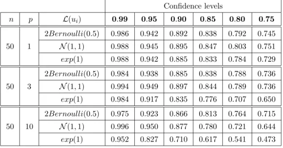
Table 2.1 shows the effective coverage probabilities of the quantiles estimated using the multiplier bootstrap. The second line contains the range of the nominal confidence levels: 0.99, . . . ,0.75 . The first left column shows the sample size n and the second column - the parameter’s dimension p. The third left column describes the distribution of the bootstrap weights: 2Bernoulli(0.5) , N(1,1) or exp(1) . Below its 2 -nd line the table contains the frequencies of the event: “the real likelihood ratio ≤ the quantile of the bootstrap likelihood ratio”.

Table 2.1: Coverage probabilities for the correct model Confidence levels n p L(ui) 0.99 0.95 0.90 0.85 0.80 0.75 50 1 2Bernoulli(0.5) 0.986 0.942 0.892 0.838 0.792 0.745 N(1,1) 0.988 0.945 0.895 0.847 0.803 0.751 exp(1) 0.988 0.942 0.885 0.833 0.784 0.729 50 3 2Bernoulli(0.5) 0.984 0.938 0.885 0.838 0.788 0.736 N(1,1) 0.994 0.949 0.897 0.844 0.789 0.736 exp(1) 0.984 0.917 0.835 0.776 0.707 0.650 50 10 2Bernoulli(0.5) 0.975 0.923 0.866 0.813 0.764 0.715 N(1,1) 0.996 0.950 0.877 0.780 0.721 0.644 exp(1) 0.952 0.827 0.710 0.617 0.541 0.473

2.4.2 Linear regression with misspecified heteroscedastic errors Here we show on a linear regression model that the quality of the confidence sets obtained by the multiplier bootstrap procedure is not significantly deteriorated by

(39)

misspecified heteroscedastic errors. Let the data be defined as Yi = Ψi>θ0 +σiεi,

i= 1, . . . , n. The i.i.d. random variables εi ∼Laplace(0,2−1/2) are s.t. IE(εi) = 0 ,

Var(εi) = 1 . The coefficients σi are deterministic: σi def

= 0.5{4−i (mod 4)}. The regressors Ψi are the same as in the experiment 2.4.1. The quasi-likelihood function

is also the same as in the previous section: L(θ) = −Pn

i=1(Yi−Ψi>θ)2/2 , and it

is misspecified, since it corresponds to σiεi ∼ N(0,1) . The target point θ∗ =θ0,

therefore, the modelling bias term kH₀−1B₀2H₀−1k from the (SmB) condition equals to zero.

Here we also consider three different parameter’s dimensions: p= 1,3,10 with

θ0 = (1, . . . ,1)>∈IRp. Table 2.2 describes the 2 -nd experiment’s results similarly to

the Table 2.1.

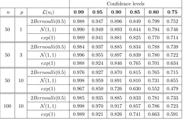
Table 2.2: Coverage probabilities for case of misspecified heteroscedastic noise Confidence levels n p L(ui) 0.99 0.95 0.90 0.85 0.80 0.75 50 1 2Bernoulli(0.5) 0.988 0.947 0.896 0.849 0.799 0.752 N(1,1) 0.990 0.949 0.893 0.844 0.794 0.746 exp(1) 0.989 0.941 0.881 0.825 0.770 0.714 50 3 2Bernoulli(0.5) 0.984 0.937 0.885 0.834 0.788 0.739 N(1,1) 0.996 0.955 0.897 0.839 0.780 0.722 exp(1) 0.988 0.924 0.846 0.765 0.701 0.634 50 10 2Bernoulli(0.5) 0.976 0.927 0.870 0.815 0.765 0.715 N(1,1) 0.998 0.959 0.891 0.810 0.731 0.655 exp(1) 0.967 0.850 0.726 0.630 0.552 0.479 100 10 2Bernoulli(0.5) 0.985 0.935 0.885 0.833 0.781 0.733 N(1,1) 0.998 0.970 0.917 0.857 0.786 0.723 exp(1) 0.989 0.921 0.826 0.741 0.663 0.591

One can see from the Tables 2.1 and 2.2 that the bootstrap procedure does a good job even for small or moderate samples like 50 or 100 if the parameter dimension is not too large. The results are stable w.r.t. the noise misspecification.

The Rademacher and Gaussian weights demonstrate nearly the same nice perfor-mance while the procedure with exponential weights tends to underestimate the real quantiles. This effect becomes especially prominent when the parameter dimension grows to 10.

(40)

26 2.4. Numerical results

2.4.3 Biased constant regression with misspecified errors

In the third experiment we consider biased regression with misspecified i.i.d. errors:

Yi=βsin(Xi) +εi, εi∼Laplace(0,2−1/2), i.i.d,

Xi are equidistant in [0,2π].

Taking the likelihood function L(θ) =−Pn

i=1(Yi−θ)2/2 yields θ

∗

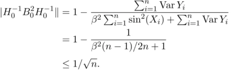
= 0 . Therefore, the larger is the deterministic amplitude β >0 , the bigger is bias of the mean constant regression. The (SmB) condition reads as

kH₀−1B₀2H₀−1k= 1− Pn i=1VarYi β2Pn i=1sin2(Xi) +Pni=1VarYi = 1− 1 β2₍_n₋₁₎_/₂_n_{+ 1} ≤1/√n.

Consider the sample size n= 50 , and two cases: β = 0.25 with fulfilled (SmB)

condition and β = 1.25 when (SmB) does not hold. Table 2.3 shows that for the large bias quantiles yielded by the multiplier bootstrap are conservative. This

Table 2.3: Coverage probabilities for the noise-misspecified biased regression Confidence levels

n L(ui) β 0.99 0.95 0.90 0.85 0.80 0.75

50 N(1,1) 0.25 0.98 0.94 0.89 0.84 0.79 0.74 1.25 1.0 0.99 0.97 0.94 0.91 0.87

conservative property of the multiplier bootstrap quantiles is also illustrated with the graphs in Figure 2.1. They show the empirical distribution functions of the likelihood ratio statistics L(eθ)−L(θ∗) and Lab(eθ

ab

)−Lab(θe) for β = 0.25 and β = 1.25 . On

the right graph for β = 1.25 the empirical distribution functions for the bootstrap case are smaller than the one for the Y case. It means that for the large bias the bootstrap quantiles are bigger than the Y quantiles, which increases the diameter of the confidence set based on the bootstrap quantiles. This confidence set remains valid, since it still contains the true parameter with a given confidence level.

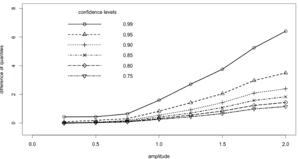
Figure 2.2 shows the growth of the difference between the quantiles of Lab(eθ

ab )− Lab(θe) and L(θe)−L(θ∗) with increasing β for the range of the confidence

(41)

Figure 2.1: Empirical distribution functions of the likelihood ratios

Yi = 0.25 sin(Xi) +Lap(0,2−1/2), n= 50 Yi = 1.25 sin(Xi) +Lap(0,2−1/2), n= 50

empirical distribution function of L(eθ)−L(θ∗) estimated with 104 Y samples

50 empirical distribution functions of Lab(eθ

ab

)−Lab(θe) estimated with 104

{ui} ∼exp(1) samples

Figure 2.2: The difference “Bootstrap quantile”−“Y -quantile” growing with modelling bias

(42)

28 2.5. Conditions

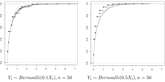
2.4.4 Logistic regression with bias

In this example we consider logistic regression. Let the data come from the following distribution:

Yi ∼Bernoulli(βXi), Xi are equidistant in [0,2], β ∈(0,1/2].

Consider the likelihood function corresponding to the i.i.d. observations:

L(θ) =Xn i=1 n Yiθ−log(1 + eθ) o .

By definition (1.3) θ∗ = log{β/(1−β)}, bigger values of β induce larger modelling bias. Indeed, the (SmB) condition reads as:

kH₀−1B2₀H₀−1k= β 2Pn i=1(Xi−1)2 nβ2₊_β₍₁₋₂_β₎Pn i=1Xi (2.9) = β 1−β · n+ 1 3(n−1) (2.10) ≤1/√n. (2.11)

The graphs on Figure 2.3 demonstrate the conservativeness of bootstrap quantiles. Here we consider two cases: β = 0.1 and β = 0.5 . Similarly to the Example 2.4.3 in the case of the bigger β on the right graph of Figure 2.3 the empirical distribution functions of Lab(θe

ab

)−Lab(θe) are smaller than the one for L(eθ)−L(θ∗) .

2.5 Conditions

Here we state the conditions required for the main results. The conditions in Section 3.4.1 come from the general finite sample theory by Spokoiny (2012a), they are required for the results of Sections A.1 and A.2. The conditions in Section 3.4.2 are required to prove the results on multiplier bootstrap from Section 2.1. In Section A.3 we verify these conditions in detail for several examples: i.i.d. observations, generalised linear model and linear quantile regression.

2.5.1 Basic conditions

Introduce the stochastic part of the likelihood process: ζ(θ)def= L(θ)−IEL(θ) , and its marginal summand: ζi(θ)

def

= `i(θ)−IE`i(θ) .

(ED0) There exist a positive-definite symmetric matrix V02 and constants g >

0, ν0 ≥1 such that Var{∇θζ(θ∗)} ≤V02 and

sup γ∈IRp logIEexp λγ >_∇_θζ₍_θ∗ ) kV0γk ≤ν₀2λ2/2, |λ| ≤g.

(43)

Figure 2.3: Empirical distribution functions of the likelihood ratios for logistic regres-sion

Yi ∼Bernoulli(0.1Xi), n= 50 Yi∼Bernoulli(0.5Xi), n= 50

empirical distribution function of L(eθ)−L(θ∗) estimated with 104 Y samples

50 empirical distribution functions of Lab(eθ

ab

)−Lab(eθ) estimated with 104

{ui} ∼exp(1) samples

(ED2) There exist a constant ω≥0 and for each r>0 a constant g2(r) such that

it holds for all θ∈Θ0(r) and for j = 1,2

sup γj∈IRp kγjk≤1 logIEexp λ ωγ > 1D −1 0 ∇2θζ(θ)D −1 0 γ2 ≤ν₀2λ2/2, |λ| ≤g2(r).

(L0) For each r∈[0,r0] (r0 comes from condition (A.2)of Theorem A.1) there

exists a constant δ(r)∈[0,1/2] s.t. for all θ∈Θ0(r) it holds

kD₀−1D2(θ)D₀−1−Ipk ≤δ(r),

where D2(θ)def= −∇2

θIEL(θ), Θ0(r) def

= {θ :kD0(θ−θ∗)k ≤r}. (I) There exists a constant a>0 s.t. a2D₀2≥V₀2.

(Lr) For each r>r0 there exists a value b(r)>0 s.t. rb(r)→+∞ for r→+∞

and ∀θ:kD0(θ−θ∗)k=r it holds

(44)

30 2.5. Conditions

2.5.2 Conditions required for the bootstrap validity

(SmB) There exists a constant δ2

smb ∈[0,1/8] such that it holds for the matrices H₀2, B₀2 defined in (1.9) and (1.10).

kH₀−1B₀2H₀−1k ≤δ_smb2 ≤Cpn−1/2.

(ED2m) For each r>0, i= 1, . . . , n, j= 1,2 and for all θ∈Θ0(r) it holds for

the values ω≥0 and g2(r) from the condition (ED2): sup γj∈IRp kγjk≤1 logIEexp λ ωγ > 1D−01∇ 2 θζi(θ)D0−1γ2 ≤ ν 2 0λ2 2n , |λ| ≤g2(r).

(L0m) For each r>0, i= 1, . . . , n and for all θ ∈Θ0(r) there exists a constant

Cm(r)≥0 such that

kD−₀1∇2

θIE`i(θ)D0−1k ≤Cm(r)n−1.

(I_B) There exists a constant a2_B≥0 s.t. a2_BD2₀ ≥B₀2.

(SD1) There exists a constant 0≤δv2 ≤Cp/n. such that it holds for all i= 1, . . . , n with exponentially high probability

H −1 0 n ∇_θì(θ∗)∇θì(θ∗)>−IE h ∇_θì(θ∗)∇θì(θ∗)> io H₀−1 ≤δ 2 v.

(Eb) The bootstrap weights ui are i.i.d., independent of the data Y , and

IEui= 1, Varui = 1,

logIEexp{λ(ui−1)} ≤ν02λ2/2, |λ| ≤g.

2.5.3 Small modelling bias condition for some models

Here we consider what becomes with the condition (SmB) for some particular models. If the observations Y1, . . . , Yn are i.i.d., then ∇θIEL(θ∗) = n∇θIE`i(θ∗) = 0 , and

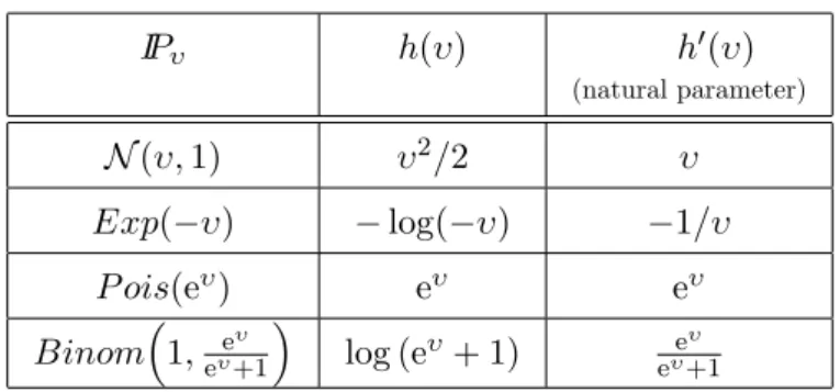
B₀2= 0 . The next example is the generalized linear model: the parametric probability distribution family {IPυ} is an exponential family with a canonical parametrisation.

The log-density for this family can be expressed as

`(υ) =yv−h(υ)

Bootstrap confidence sets under model misspecification

model misspecification

D i s s e rtat i o n

zur Erlangung des akademischen Grades

Dr. Rer. Nat.

im Fach Mathematik

eingereicht an der

Mathematisch-Naturwissenschaftlichen Fakult¨

at

Humboldt-Universit¨

at zu Berlin

von

Dipl.-Math. Mayya Zhilova

Pr¨

asident der Humboldt-Universit¨

at zu Berlin:

Prof. Dr. Jan-Hendrik Olbertz

Dekan der Mathematisch-Naturwissenschaftlichen Fakult¨

at:

Prof. Dr. Elmar Kulke

Gutachter:

1. Prof. Dr. Vladimir Spokoiny

2. Prof. Dr. Gilles Blanchard

3. Prof. Dr. Victor Chernozhukov

eingereicht am: 30. Juni 2015

Contents

Introduction

1.1

Likelihood-based confidence sets

1.2

Multiplier bootstrap procedure for the case of one

parametric model

1.3

Theoretical justification of the bootstrap for the case

of one parametric model

1.4

Simultaneous confidence sets

1.5

Notation

1.6

Organization of the thesis

Bootstrap likelihood-based

confidence sets

2.1

Multiplier bootstrap procedure

2.2

Main results

2.3

Smoothed version of a quantile function

2.4

Numerical results

2.5

Conditions