Kernel based nonparametric coefficient estimation in diffusion models

(1)

Kernel Based Nonparametric

Coefficient Estimation in Diffusion

Models

Dissertation

zur Erlangung des akademischen Grades

Doctor rerum naturalium

(Dr. rer. nat.)

vorgelegt

der Fakult¨at f¨ur Mathematik

der Technischen Universit¨at Dortmund

von

Dipl.-Math. Benedikt Funke

(2)

Datum der m¨undlichen Pr¨ufung 18.11.2015

Ver¨offentlichte Fassung vom 25.11.2015

(3)

Acknowledgments

For the successful completion of this thesis, I firstly wish to thank my advisor Prof. Dr. Jeannette H.C. Woerner. She suggested this interesting topic to me and gave me constant support and inspiration by interesting and constructive discussions throughout the devel-opment of this thesis. Beyond that, she always encouraged me to participate at several different workshops and, thereby, offered me the possibility to meet colleagues from di-versified fields of stochastics and statistics.

Moreover, I am deeply grateful for the financial support and the fruitful research environ-ment by the Collaborative Research Center “Statistical modeling of nonlinear dynamic processes” (SFB 823) of the German Research Foundation (DFG), through which I also came in contact with Prof. Herold Dehling.

I also wish to thank my colleagues from the sixth floor Daniel Kobe, Sven Glaser, and Christian Palmes for their assistance, friendship and for sharing many happy and enjoy-able times.

Finally, I wish to thank my family for supporting me all the time. Last but not least, I wish to thank Fabienne for her love and her tireless support.

(4)

(5)

1 Introduction

1.1 Motivation

The present thesis mainly focuses on nonparametric estimation methods for certain classes of stochastic processes. It is divided into three main subject areas. We start with the formulation of a kernel based nonparametric estimation procedure for jump diffusions. Afterwards we will focus on bias reduction techniques for this class of estimators. Finally, we will work with multivariate models and introduce the concept of copula functions. As already mentioned, the first part deals with nonparametric kernel estimators for solu-tions of stochastic differential equasolu-tions. We will start with a model based on a Brownian motion driven diffusion process as a motivation and will afterwards mainly deal with jump diffusions. Nonparametric kernel estimation for the coefficients of jump diffusions has not attracted much attention in the literature, yet. Most of the existing articles are concerned with the case of an additive independent finite activity jump process, which means -roughly speaking- that they focus on compound Poisson processes as a source of additive jumps. We will extend the existing results to the case of L´evy-driven jump diffu-sion models. The class of L´evy processes provides many possibilities of modeling certain jump behavior of, for instance, economic processes like stock prices, volatilities or interest rates.

We propose Nadaraya-Watson like estimators based on kernel functions as well as a band-width and will explore their asymptotic properties, i.e., consistency and asymptotic nor-mality. The latter allows us to construct pointwise asymptotic confidence intervals, which are very useful for practical issues.

Based on these results, we will subsequently extend them to the case of noisy data. This kind of data plays a significant role, especially in high frequency settings; see for exam-ple Jones (2003) and Zhou (1996). In particular, we will not observe the diffusion itself but rather a sample containing an additive white noise process. Using a pre-averaging approach, we are able to get rid of the noise and make use of the asymptotic results in the non-noisy case.

The last section of the first part contains another example of a very interesting and, for practical issues, relevant jump diffusion model. Particularly, we will focus on integrated jump diffusion processes. These processes appear naturally in problems of engineering and physics. One can, for example, think of a velocity of a particle as the original jump diffusion process and the coordinate of the particle as the integral up to a fixed time point

t _≥0. Moreover, we assume that we are only able to observe the coordinate whereas the velocity is hidden. Making again use of the pre-averaging approach, we see that under appropriate assumptions, the results of the first section can also be used in this context. The second part is mainly concerned with bias reduction techniques for

(8)

nonparamet-ric kernel based estimators. We will start with an adaptive version of the well-known Nadaraya-Watson estimator for nonparametric regression estimation. We will see that an appropriate choice of the newly introduced bandwidth function will asymptotically lead to a significant reduction of the order of the bias term. We show that this appealing property withstands even under weak dependency of the available sample. For our proofs we will make use of techniques borrowed from classical discrete time series analysis and will afterwards construct an adaptive drift estimator for a continuous diffusion process in view of the discrete findings.

Subsequently, we will leave the univariate case and focus on multivariate stochastic pro-cesses. We will especially deal with the so-called “boundary bias” effect, which occurs when we want to estimate densities possessing bounded or compact support by the use of symmetric kernel based estimators. The effect describes, for instance, the fact that symmetric kernel based estimators smear over probability mass to the negative real line or outside the unit square, although the corresponding densities are only supported on

R+ _{or respectively on [0}_,_1]2_{. This problem has been attained a lot of attention in the}

literature and many methods for avoiding this effect have been published. We will focus on an approach by Chen (1999, 2000), who uses asymmetric probability densities like Beta and Gamma kernels for the estimation of unknown univariate densities. Furthermore, we will develop an extension of this approach due to the multivariate case and will afterwards introduce two non-negative multiplicative bias correction methods improving the rate of the bias term significantly. We explore bias and variance approximations and focus on several choices for the kernel functions. Regression estimators based on this method are then suggested for the estimation of the drift vector of a multivariate diffusion process. The last section mainly focuses on the estimation of compact supported densities. Partic-ularly, we will look at densities whose support is the unit hyper cube [0,1]d_{and construct} nonparametric estimators via the use of Bernstein polynomials. In the literature, this approach has been used for the estimation of copula densities. We will briefly introduce the class of copula functions and will afterwards introduce various estimation approaches. Finally, due to Sklar´s theorem, we are able to represent conditional densities as well as conditional expectations in terms of the corresponding copula densities. This represen-tation will lead us to the use of a Bernstein polynomial based estimator for conditional expectations which are in contrast -as we have already seen- approximations for the un-known drift and diffusion coefficient in diffusion models. Hence, this gives us another possibility to face the problem of estimating unknown conditional expectations or regres-sion functions.

1.2 Preliminaries and basic notations

In this section we will shortly introduce our used notations and will define the basic tools for our subsequent analysis. There exists a variety of useful books introducing the

(9)

concept of stochastic processes. We only refer to those definitions being useful and in any way needed for our following analysis. For this purpose we restrict ourselves to the most important definitions and tools given in the books by Karatzas and Shreve (1996) as well as Cont and Tankov (2004). The following section is based on their introduction chapters. We will subsequently work on a filtered probability space (Ω,_A,(_At)t_≥0, P) where A

denotes a σ-algebra, (At)t_≥0 a filtration of sub-σ-algebras, and P a probability measure.

A stochastic process X = (Xt(ω))t_≥0 := (Xt)t≥0 is a family of random variables, which

means that Xt is a random variable for every t ≥ 0. We omit the dependency of the randomness ω, but always keep in mind that we work on a probability space. Moreover, a process X is called adapted to (At)t_≥0, if Xt is At measurable for all t ≥0.

For a fixed ω _∈ Ω, the map t _→ Xt(ω) is called a path of the process X. During our following analysis, we will always observe a discrete sample of a path of an underlying stochastic process and will construct estimators for characteristics of this process based on this sample.

Another mentionable definition are the Lp_(Ω_,_A_{, P}_{) :=} _Lp₍_P_{) spaces. We say that a} random variable X: Ω→Rd _{belongs to}_Lp₍_P_{), if}

E[_|X_|p] = Z Ω| X(w)_|pdP(w) = Z Rd| x_|pPX(dx)<_∞, where PX(A) =P(X−1(A)), A_{∈ B}(Rd₎

denotes the image measure of X.

A very important class of stochastic processes, which additionally plays a major role in the following chapters, are martingales. We will omit the concept in terms of discrete time and will restrict ourselves to the continuous-time case. We will at first introduce the Brownian motion, which acts as a fundamental stochastic process and is also very important in the context of diffusion processes, which will play a central role within this work later on. For the sake of simplicity, we will restrict ourselves to the case d= 1.

Definition 1.1. A one-dimensional Brownian motion W = (Wt)t_≥0 on a filtered

proba-bility space (Ω,_A,(_At)t_≥0, P) is an adapted stochastic process fulfilling

a) W has independent increments, which means that Wt−Ws is independent of As,

for s≤t,

b) W has stationary increments, which are normally distributed such that

Wt−Ws=D N(0, t−s),

c) W has almost surely continuous paths and

(10)

A Brownian motion is one basic example of a continuous-time martingale. Other examples of martingales will become very important later on. For this purpose let us now define another fundamental class of stochastic processes, namely the class of Lévy processes. These processes play a central role in many scientific fields. Applications can be found for instance in physics (analysis of turbulence data), in engineering (construction of dams protecting the environment against flood catastrophes), in economics as a toy-example of a discontinuous asset price, and, of course, in mathematical finance (in particular in risk theory). Several advisable books introduce the interested reader into this field of stochastic processes. We refer to Sato (1999), Cont and Tankov (2003), and Barndorff-Nielsen et al. (2001). A very useful survey about Lévy processes and their applications in finance has been published by Papapantoleon (2008), from which the ideas how to introduce Lévy processes in the following way are extracted.

We start with a formal definition of a L´evy process and concentrate only on the one-dimensional case due to the sake of simplicity.

Definition 1.2. A real-valued, adapted, and càdlàg (French “continue à droite, limite à

gauche”; English RCLL: “right continuous with left limits”) stochastic processL= (Lt)t≥0

on a filtered probability space(Ω,_A,(_At)t_≥0, P)such thatL0 = 0a.s. is called L´evy process,

if

a) L has independent increments, which means that Lt −Ls is independent of As,

0≤s < t,

b) L has stationary increments, i.e., the distribution of Lt+h −Lt is independent of t

for all h >0 and

c) L is stochastically continuous, i.e.

∀ε >0 : lim

t→sP(|Lt−Ls|> ε) = 0, for every t≥0.

The literature features different definitions for L´evy processes. The definition above seems to be most adequate for our purposes, because the handling of small increments of stochas-tic processes will play a central role in our subsequent analysis; see c) in Definition 1.2.

Example 1.3. The easiest examples of L´evy processes are given by a deterministic linear

drift Lt = at, a ∈ R, by the Brownian motion Lt = Wt, and by a (compound) Poisson

process.

A fundamental characterization of L´evy processes provides the L´evy-Khintchine repre-sentation of the corresponding characteristic function of L. Due to its importance, we will state this result here. Further, it acts as an elegant tool for the derivation of higher moments of L and will be important subsequently.

(11)

Theorem 1.4(Cont and Tankov (2003), Theorem 3.1).LetL= (Lt)t_≥0 be a L´evy process,

then there exists a triplet (b, σ, ν) where b _∈ R_{, σ} _∈ R+ _{and additionally} _ν _{is a measure}

on R _fulfilling

ν(_{0_}) = 0 and

Z

R

(1_∧x2)ν(dx)<_∞

such that the characteristic function of Lt can be represented as

ϕLt(u) :=E[e iuLt_{] = exp} t ibu₋ u 2_σ 2 + Z R eiux₋1₋iux1_{|x|≤1} ν(dx) . Remark 1.5. This representation does not only hold for L´evy processes but rather for the characteristic function of a random variable whose distribution is infinitely divisible.

We do not go into detail here, but remark that the law of Lt is infinitely divisible and (in

turn) for every infinitely divisible random variable X one can construct a L´evy process L˜

such that L˜1 =D X.

We will now introduce the concept of Poisson random measures of L´evy processes, which provide a very useful tool to work with these processes by using martingale techniques under appropriate assumptions.

Definition 1.6. Let L= (Lt)t_≥0 be a L´evy process and ∆L:= (∆Lt)t≥0 := (Lt−Lt−)t≥0

the corresponding pure jump process, where Lt− := lims↑tLs. Let B ∈ B(R\{0}) a Borel

set such that 0∈/ B, where B denotes the closure of the Borel set B. We set

µL(ω, t, B) := #{0≤s ≤t: ∆Ls∈B}= X

0≤s≤t

1B(∆Ls)

and call µL _{the Poisson random measure of} _L_.

Roughly speaking, µL _{is the non-negative integer-valued random measure, which counts} the jumps of Lup to a certain time t such that ∆Ls∈B.

The name Poisson random measure is justified by the following observations (cf. Papa-pantoleon (2008)):

a) µL _{has independent increments, which means that} _µL₍_{ω, t, B}₎₋_µL₍_{ω, s, B}_{) is} inde-pendent of _As. This can be seen in the fact that

µL(ω, t, B)₋µL(ω, s, B)_∈σ(_{Lu−Lv; s≤v < u≤t}) and that L has independent increments.

b) µL _{has stationary increments because}

µL₍_{ω, t, B}₎₋_µL₍_{ω, s, B}_{) = #}_{₀_≤_u_≤_s₋_t_{: ∆(}_L

s+u−Ls)∈B} and that L has stationary increments.

(12)

Hence, (µL(ω, t, B))t_≥0 is a non-negative integer-valued L´evy process whose jumps are all

of height 1. Consequently, µL _{is, for a fixed Borel set} _B _{and indexed in} _t _≥ _{0, a Poisson} process with intensity

ν(B) := E[#_{0_≤s_≤1 : ∆Ls ∈B}], which means that

P(µL(ω,_·, B) = k) = e−ν(B)ν(B)

k

k! , ∀k ∈N0.

For further reading on this topic, we refer to Cont and Tankov (2004), Section 2.6.

ν is called the Lévy measure or the Lévy density of L and has already been used in the Lévy-Khintchine representation as well as in the characteristic triplet.

The L´evy measure provides information about the expected number of jumps of a certain height within a time interval of length 1. Since RR(1∧x

2₎_ν₍_dx₎ _< _∞_{, the L´evy process}

L can have infinitely many small jumps, but does only have finitely many jumps of size

J _≥1. A L´evy process is called infinitely active when ν(R_{) =} _∞_{. Finite activity processes}

(ν(R₎ _< _∞_{) are, in general, compound Poisson processes and will not play a significant}

role in our following analysis.

We now state another fundamental representation of a Lévy process, namely the Lévy-Itô decomposition where Poisson random measures as well as the Lévy measure appear, too.

Proposition 1.7 (Cont and Tankov (2004), Proposition 3.7). Let L= (Lt)t_≥0 be a L´evy

process with Poisson random measure µL _{and characteristic triplet} ₍_{b, σ, ν}₎_{. Then,} _L _can

be decomposed into the sum of four independent L´evy processes L(i)_{, i} _{= 1}_{, ...,}₄_{, in the}

following way Lt=L(1)t +L (2) t +L (3) t +L (4,ε) t =bt+√σWt+ Z t 0 Z {|x|≥1} xµL(ds, dx) + lim ε↓0 Z t 0 Z {ε<|x|<1} x(µL−νL)(ds, dx) =:bt+√σWt+ X 0<s≤t ∆Ls1_{|∆Ls|≥1}+ Z t 0 Z {|x|<1} x(µL(ds, dx)−ν(dx)ds),

where L(1) _{is a linear drift term,} _L(2) _{is a scaled Brownian motion,} _L(3) _{is a compound}

Poisson process with arrival rateλ=R_{|_x_|≥₁_}ν(dx), andL(4) _{:= limε}

↓0L(4,ε)is a pure jump

martingale.

The fact that the last part L(4) _{is a martingale can be seen for instance through}

Propo-sition 2.16 in Cont and Tankov (2004). Moreover, the reason why we stated this decom-position here is that we will work with diffusions driven by L´evy processes, which are time-continuous martingales. Additionally, we assume that the driving L´evy process pos-sesses finite moments of certain orders. The relation between the existence of moments of

(13)

Proposition 1.8 (Cont and Tankov (2004), Proposition 3.13). Let L= (Lt)t_≥0 be a L´evy

process with triplet (b, σ, ν), then

E[_|Lt|n]<∞ ⇔ Z

{|x|≥1}|

x_|nν(dx)<_∞.

In this case, the moments can be deduced in a rather simple way by differentiation of the characteristic function. In particular, we can state that

E[Lt] =t b+ Z {|x|≥1}| x_|ν(dx) as well as V ar(Lt) =t σ+ Z R x2ν(dx) .

Finally, we want to conclude the mentioned properties of L´evy processes and use them for our purposes. In the following section, we will work with a L´evy processL of the form

Lt= Z (0,t] Z R x(µL(ds, dx)−ν(dx)ds) := Z t 0 Z R x(µL(ds, dx)−ν(dx)ds) := Z t 0 Z R xµ¯L(ds, dx) possessing the property that RRx

4_ν₍_dx₎_<_∞_{. ¯}_µL _{denotes the compensated Poisson} ran-dom measure of L. We are able to rewrite L in view of the L´evy-Itˆo decomposition as follows: Lt= Z t 0 Z R x(µL(ds, dx)₋ν(dx)ds) = Z t 0 Z {|x|<1} x(µL(ds, dx)−ν(dx)ds) + Z t 0 Z {|x|≥1} xµL(ds, dx) − Z t 0 Z {|x|≥1} xν(dx)ds :=L(3)+L(4)+ ˜bt, where ˜b:=−R_{|_x_|≥₁_}xν(dx)∈R_.

Hence, L has the triplet (˜b,0, ν) and is a martingale possessing a finite fourth moment

E[L4_t] =t 3 Z R y2ν(dy) 2 + Z R y4ν(dy) ! .

In addition, the characteristic function ϕLt(u) ofL is given by

ϕLt(u) =E[e iuLt_{] = exp} t Z R (eiux−1−iux)ν(dx) .

(14)

2 Nonparametric drift estimation in a L´

evy-driven

diffusion model

2.1 First intuitions in scalar diffusion models

In this chapter we will focus on the nonparametric estimation of the coefficients in a certain jump diffusion model. To motivate our procedure, we will at first have a look at an ordinary diffusion model driven by a Brownian motion. To be precise, consider a filtered probability space (Ω,_F,(_FW

t )t≥0, P) equipped with a Brownian MotionW = (Wt)t≥0 and

the canonical filtration_FW

t :=σ(Ws, s≤t). LetX = (Xt)t≥0 be a diffusion process given

by the time-homogeneous stochastic differential equation

dXt =b(Xt)dt+σ(Xt)dWt, X0 =D η,

where b and σ >0 are unknown functions, which are globally Lipschitz-continuous such that the equation possesses a pathwise unique strong solution (see Karatzas and Shreve (1996), Proposition 2.13). Moreover, let the initial condition η _∈ L2₍_P_{) be independent}

of W. Now define

Ft:=σ(η, Ws; 0≤s≤t), 0≤t ≤ ∞ and additionally the “collection of null sets”

N :=N∞ :={N ⊂Ω;∃F ⊂ F∞ with N ⊂F and P(F) = 0}.

We call

FtX :=σ(Ft∪ N)

the augmented filtration fulfilling the usual assumptions. This means that it is complete and right-continuous (see Karatzas and Shreve (1996), Proposition 7.7). The solution

Xt =X0+ Z t 0 b(Xs)ds+ Z t 0 σ(Xs)dWs is_FX

t adapted and also a semimartingale. Furthermore, the process is determined by the functions b and σ and, hence, it seems natural to be interested in their behavior and shape. By additional assumptions within this model, which cause that X is stationary and equipped with a stationary density, one can see that this density can explicitly be represented only in dependence of b and σ2_{; see for example Karatzas and Shreve (1996),}

pp. 352.

Due to the importance of the drift b and the volatility σ, several different approaches for the (non-)parametric estimation of diffusion models have been published. In this work we are only interested in nonparametric approaches. For parametric estimation procedures, we refer to a recently published book by Kessler et al. (2012).

(15)

In the nonparametric setting, any list of existing methods would be incomplete, so we will only mention those approaches playing a significant role for our subsequent analysis. Very fundamental and crucial work has been done by Comte and Genon-Catalot; see for instance Comte et al. (2009), (2010) and Comte and Genon-Catalot (2007). Their approach is based on model selection and provides an adaptive estimator for both, the drift and the volatility function, for which the L2_{-risk can be bounded dependent on the}

smoothness of these functions as well as the sampling frequency. Due to the adaptivity of their estimator, an asymptotic distribution is not derivable and, therefore, confidence intervals cannot be determined. Nevertheless, simulation issues reveal that their estimators provide good results. Later on, we will compare our findings with those of Schmisser (2014), who developed the same estimation procedure as Comte and Genon-Catalot in a jump diffusion setting.

In contrast to the upper approach, other authors focused on kernel based estimation of diffusion models. Their findings will act as a basis for our approach in the L´evy-driven model. In this context, very important work has been done by Bandi. His articles provide a complete asymptotic analysis of kernel based estimators for ordinary diffusion models; see Bandi and Phillips (2001), (2003). He also extends his results to jump diffusion models driven by compound Poisson processes and to multivariate diffusion models; see Bandi and Nguyen (2003) as well as Bandi and Moloche (2008). Due to the importance of his results, we will briefly describe the motivation behind a kernel based approach below. To develop nonparametric estimators for b and σ, Stanton (1997) uses approximations of the infinitesimal generator L of X defined by

L(f)(x, t) := lim τ↓t E[f(Xτ, τ)|Xt =x]−f(x, t) τ ₋t = ∂f(x, t) ∂t + ∂f(x, t) ∂x b(x) + 1 2 ∂2_f₍_{x, t}₎ ∂x2 σ 2₍_x₎_.

The last equation is a classical result for Itˆo-diffusions and can, for instance, be found in Øksendal (2000, Theorem 7.3.3). For our purposes, it is sufficient to assume that f ∈ C2

0(R×R+). Under this assumption, the above limit exists and is therefore contained

in the domain of L. Using a Taylor expansion of f, one can finally deduce a first order approximation for the drift b (by setting ∂f_∂x(x,t) =x) and for the volatility function σ (by setting ∂f_∂t(x,t) = (x−Xt)2_{) via} b(x) = 1 ∆E[Xt+∆ −Xt|Xt=x] +O(∆), as ∆→0 σ2(x) = 1 ∆E[(Xt+∆ −Xt) 2 |Xt=x] +O(∆), as ∆→0.

We refer to Stanton (1997) for higher order approximations of b and σ. For our purposes, these approximations are sufficient and are the basis for both Bandi´s and our estimation procedure in more involved models.

(16)

Using the above approximations, it is quite intuitive to use nonparametric regression tech-niques, which are well developed for discrete time series analysis. There is a plethora of different regression estimators like local polynomial estimators, splines, jackknife estima-tors or neural networks. Due to its popularity and the well-known asymptotic properties, we focus on a local constant estimator, which is also known as the Nadaraya-Watson estimator (cf. Nadaraya (1965), Watson (1964) or H¨ardle (1990)) for the estimation of conditional moments in regression frameworks. The intuition of this estimator is to use weighted averages of infinitesimal increments of X, which lie in the vicinity of the spatial point x at which we want to estimate both functions b and σ. The quantification of the rather imprecise term “vicinity” will be handled later on. The weighting will be realized by a kernel function K which is in general a symmetric probability density function pos-sessing a finite second moment. For all following derivations, one can think of a Gaussian density as a toy-example for which all assumptions will hold true.

To further illustrate the idea of the previously described procedure, we suppose that we observe the processX at equidistant time points 0,∆,2∆, ..., n∆. An initial estimator for the drift b at point x according to the above description would be given by

ˆ_b₁₍_x_{) :=} nh1 Pn−1 i=0 1(|Xi∆−x|≤h) (X(i+1)∆−Xi∆) ∆ 1 nh Pn−1 i=0 1(|Xi∆−x|≤h) = 1 nh Pn−1 i=0 1_| Xi∆−x| h ≤1 (X(i+1)∆−Xi∆) ∆ 1 nh Pn−1 i=0 1|Xi∆−x| h ≤1 ,

whereh=hn is a bandwidth and ∆ = ∆n is the sampling frequency. The bandwidth will regulate what is meant by the term “vicinity”.

To explore asymptotic properties like consistency and the derivation of the asymptotic distribution, it seems intuitive to ensure the following points:

i) It is a well-known fact that the drift function cannot consistently be (nonparamet-rically) estimated on a compact interval; see for instance Bandi and Phillips (2003). Therefore, it seems natural to impose that n∆ := T _{→ ∞} for the examination of ˆ_b₁₍_x_).

ii) To reproduce our initial approximation of b, we have to impose that ∆ → 0 as

n_{→ ∞}.

iii) The bandwidthhhas to decrease to zero asn _{→ ∞}to ensure that only observations “near”x are included for estimating b(x).

iv) The rescaled denominator

n−1 X i=0 1_| Xi∆−x| h ≤1

has to diverge as n → ∞ in order to guarantee that the processX infinitely often hits a neighborhood of x.

(17)

Later on, we will specify all these intuitive conditions to derive the desired asymptotic properties of our proposed drift estimator.

From a heuristic point of view, it seems to be reasonable that observations near xshould be equipped with higher weights than others. Therefore, it would be a canonical approach to substitute the indicator kernel 1

|Xi∆−x| h ≤1

by a smooth kernel functionK whose basic

properties have already been mentioned. Bandi and Phillips (2003) and Bandi and Nguyen (2003) finally suggested the estimators

ˆ_b₍_x_{) :=} nh1 Pn−1 i=0 K Xi∆−x h (X(i+1)∆−Xi∆) ∆ 1 nh Pn−1 i=0 K Xi∆−x h as well as ˆ σ2(x) := 1 nh Pn−1 i=0 K Xi∆−x h (X(i+1)∆−Xi∆)2 ∆ 1 nh Pn−1 i=0 K Xi∆−x h .

They explored the strong consistency and the asymptotic normality under usual regularity assumptions on b and σ like Lipschitz-continuity and ellipticity of σ (which means that

σ(x) > σ0 > 0). Following our first intuitions, their derivations are based on the double

asymptotics scheme

∆→0 and T =n∆→ ∞.

Remark 2.1. For the consistent nonparametric estimation ofσ, the assumption T → ∞

is not necessary; see for example Florens-Zmirou (1993) or Bandi and Phillips (2003) for an exact mathematical justification of this fact. Due to this reason, the second estimator possesses a faster rate of convergence. Later on, we will see that, in contrast to the ordinary diffusion model, the double asymptotics scheme is necessary for both estimators in our considered L´evy-driven model.

2.2 Scalar jump diffusion models driven by a finite activity jump

process

To the best of our knowledge, the first paper which investigated nonparametric kernel based estimators for the coefficients in a jump diffusion model is the one by Bandi and Nguyen (2003). We will shortly present their approach and the used techniques. After that, we will use analogous arguments for the derivation in a more general model.

Adding jumps in a diffusion model seems to be very important from a practical point of view. As we want to model interest rates or stock prices, macroeconomic news, endogenous as well as exogenous shocks can cause abrupt changes during the evolution of the process

X. Hence, it is quite intuitive to include an additive (independent) jump component. Bandi and Nguyen (2003) focused on the following class of processes

dXt=b(Xt)dt+σ(Xt)dWt+ Z

(18)

where ¯ν(ds, dy) = µ(ds, dy)−Γ(dy)ds is a compensated Poisson random measure with intensity Γ(dy)ds, where Γ(dy) is a probability distribution. To coincide with their nota-tion, we set here the intensity of the underlying Poisson process equal to 1. Because of this assumption on the jump size distribution Γ(dy),Xis a process with finite activity. As a consequence, they allow for jumps occurring due to an independent additive compound Poisson process.

In the following section, we will present our main results, where we explicitly not assume that the additive jump component is of finite activity but is rather a L´evy process pos-sessing certain finite moments.

Bandi and Nguyen (2003) focused on the same double asymptotics scheme as in the Brow-nian case before and used nonparametric regression techniques for the estimation of the first and second conditional moment of infinitesimal changes of the process X. The ap-proximations of the infinitesimal generator for the above discontinuous processXare now given by (Bandi and Nguyen (2003), p.297):

b(x) = lim ∆→0 1 ∆E[Xt+∆ −Xt|Xt=x] σ2(x) +E[c2(x, Y)] = lim ∆→0 1 ∆E[(Xt+∆−Xt) 2_|_X t=x] (2.1) E[ck(x, Y)] = lim ∆→0 1 ∆E[(Xt+∆−Xt) k |Xt=x], k≥3,

where we naturally assume that the above conditional moments exist and Y = Γ(D dx) denotes the jump size distribution. This should only be understood as a motivation how we can construct Nadaraya-Watson like estimators even in this jump diffusion setting. The dependency of these approximations of the jump component is not surprising. In the jump diffusion case, the approximation of the infinitesimal generator of X can be decomposed into the approximation of the continuous part _L and the one for the discontinuous part

M, where

M(φ)(x) := Z

R

(φ(x+c(x, y))−φ(x)−φ′(x)c(x, y))Γ(dy).

Bandi and Nguyen (2003) provide an asymptotic analysis of the appropriate Nadaraya-Watson like estimators based on symmetric kernels. It should also be mentioned that a comparable semiparametric analysis has been conducted by Johannes (2004), who pro-posed estimators for the coefficients of the above mentioned jump diffusion model, too. For this purpose, he parametrized the jump size distribution and used the proposed ap-proximations to construct estimators based on the method of moments.

Remark 2.2. The results in Bandi and Phillips (2003) as well as in Bandi and Nguyen (2003) hold true even for a relatively broad class of stochastic processes. Their central

identifiability assumption is that the process X is Harris-recurrent. This ensures that X

(19)

(2003) for more details. Subsequently, we will assume that X is stationary and σ is

ellip-tical. Moreover, we weaken their assumption that b has to be bounded.

2.3 Drift estimation in a L´

evy-driven diffusion model

We now turn to our main section, namely the nonparametric estimation of the coefficients in a L´evy-driven jump diffusion model.

Let, therefore, (Ω,_F,(_Ft)t_≥0, P) be a filtered probability space equipped with a Brownian

MotionW = (Wt)t_≥0and a L´evy processL= (L(t))t≥0 = (Lt)t≥0of the already introduced

form dLt= Z R y(µ(dt, dy)₋ν(dy)dt) := Z R yµ¯(dt, dy),

where µis a Poisson random measure compensated by its intensity measure ν(dy)dt. We assume that the L´evy measure ν(dy) satisfies

E[L2(1)] =V ar(L(1)) = Z

R

y2ν(dy)<_∞.

The representation ofV ar(L(1)) by its corresponding L´evy measure can easily be derived by differentiation of the characteristic function as it was presented in the introduction. We remark that L is a martingale with respect to its canonical filtration and possessing finite variance.

Now consider a stochastic process X = (Xt)t_≥0 such that

dXt =b(Xt)dt+σ(Xt)dWt+ξ(Xt−)dLt, X0 =D η, (2.2)

whereb,σandξare unknown functions andX possesses the initial distributionη= Γ(D dx). We also assume that W and L are independent processes and that η _∈ L2_(Γ(_dx_{)) is}

independent ofW as well asL. In addition, we choose as filtration_Ft :=σ(η,(Ls, Ws), s≤

t) such that Xt is Ft adapted. We should remark that the integral

Zt:= Z t 0 Z R ξ(Xs−)yµ¯(ds, dy)

denotes a martingale with respect toFt and satisfies the isometry formula

E[Z_t2] =E Z t 0 Z R ξ2(Xs)y2ν(dy)ds .

Furthermore, by imposing that ξ is bounded (cf. Assumption A1,ii)), we easily conclude that E Z t 0 Z R ξ2(Xs)y2ν(dy)ds ≤t_||ξ2_||_∞ Z R y2ν(dy).

(20)

Moreover, Xt− denotes the c`agl`ad version of the process X which ensures that the

in-tegrand is a predictable process such that the stochastic integral can be defined in the usual manner; see Cont and Tankov (2004), Section 8.1.4. for further details on stochas-tic integrals with respect to Poisson random measures. Suppose that we observe X in a high frequency setting on the interval [0, T] on an equidistant grid at time points 0,∆,2∆, ..., n∆ = T. Our first aim will be the construction of a meaningful pointwise estimator of the drift function b at a design point x based on the available sample

X0, X∆, X2∆, ..., Xn∆ =XT.

This problem originates from Schmisser (see Schmisser (2013), (2014)), who proposed adaptive nonparametric estimators for bas well asσ2₊_{V ar}₍_L₍₁₎₎_ξ2 _{on a compact subset}

A_⊂R_{by the use of a model selection approach. Our procedure differs substantially from}

this technique, as we are interested in pointwise estimators. Moreover, we are concerned with kernel based estimators for which we incorporate an additional regularization pa-rameter, namely the bandwidthh. To the best of our knowledge, there is no work done yet covering the nonparametric estimation ofb(x) in a L´evy-driven diffusion model. It should be mentioned that for the nonparametric estimation ofσ2₍_x_{) in an infinite activity model,}

there is a reasonable and alternative approach by Mancini and Ren´o (2011). They used a threshold estimator, which disentangles the discontinuous from the continuous part of the process X. The new thinned out sample is used for the construction of an estima-tor of σ2₍_x_{). In contrast to our approach, they are only interested in the fixed} _T _case,

namely when one observes the process X only on a compact interval of the form [0, T]. Their estimator converges with rate√nh. Furthermore, and to the best of our knowledge, minimax rates for b, σ and ξ are not available in the literature, yet. We are now ready to list our assumptions on the considered model, which will lead us to the first very useful proposition.

Assumption A1

i) The functions b, σ and ξ are globally Lipschitz-continuous.

ii) The functionσis bounded away from zero (ellipticity condition) as well as uniformly bounded for all x:

∃ σ1, σ0 ∈R:∀x∈R: 0 < σ1 ≤σ(x)≤σ0.

iii) The function ξ is non-negative and also bounded:

∃ ξ0 ∈R:∀x∈R: 0≤ξ(x)≤ξ0.

iv) The function b is elastic (cf. Masuda (2007)). This means that

(21)

where the relation . is defined as follows:

let S be a set and f, g :S _→[0,_∞) two functions. Then,

f .g :⇔ ∃C ∈R+ _: _f₍_x₎_≤_C_·_g₍_x₎ _∀_x_∈_S.

Especially, b cannot be bounded as required in Bandi and Nguyen (2003). v) The L´evy measure ν possesses the properties that

V ar(L(1)) = Z

R

y2ν(dy)<_∞, ν(_{0_}) = 0.

Under Assumption A1,i) a unique strong solutionX of (2.2) it exists (cf. Masuda (2007)). Moreover, under A1,i)-v), this solution is equipped with a unique invariant probability distribution Γ(dx). Moreover,X fulfills aβ-mixing condition. In general, a homogeneous Markov process X with transition semigroup (Pt)t_∈R₊ and initial distribution ηis said to

be β-mixing with coefficient βX(t), if

βX(t) := sup s∈R₊

Z

||Pt(x,·)−ηPs+t(·)||ηPs(dx)−→0, as t→ ∞,

where ηPt denotes the distribution of Xt and ||λ|| defines the total variation norm of a signed measure λ; see Masuda (2007). This mixing property describes the temporal dependence of the process. Due to Masuda (2007), X is, in addition, exponentially β -mixing, which means that there exists a constant γ >0 such that

βX(t) = O(e−γt), ast → ∞.

Using Theorem 2.1 in Masuda (2007) we can deduce the ergodicity of X, which means that for all measurable functions g _∈L1_(Γ(_dx_)):

1 T Z T 0 g(Xs)ds −→ Z R g(x)Γ(dx) a.s., as T → ∞.

For further information and especially equivalent reformulations of A1,iv), we recommend Masuda (2007).

Due to our assumptions on the L´evy measure ν and the Lipschitz-continuity of the coef-ficients b, σ and ξ, we have that E[X2

t]< ∞. This can easily be proven by applying the Cauchy-Schwarz inequality successively. We will focus on this property later on.

Moreover, we impose that

vi) Γ is absolutely continuous with respect to the Lebesgue measure and, thus, possesses a Lebesgue density π such that Γ(dx) = π(x)dx.

(22)

For sufficient conditions on A1, vi) see Ishikawa and Kunita (2006), which ensure that under our assumptions on ξ(especially the boundedness from below) a smooth transition density exists.

We remark that the process X is also stationary, because we assumed that X0 ∼Γ(dx).

These assumptions are largely congruent to those in Schmisser (2014), which make com-parisons of the derived results much easier.

We are now ready to state our first proposition. It turns out that this result is one of the key elements for our asymptotic analysis. The following result originates from Schmisser (2014) but is not proven there.

Proposition 2.3. Let X = (Xt)t≥0 be the solution of (2.2). Under assumptions A1,i)-vi)

a constant C > 0 exists, such that

E " sup |s−t|≤∆ (Xs−Xt)2 # ≤C∆, provided that ∆≤1.

For the proof of this statement, we need the following two inequalities of the Burkholder-Davis-Gundy type (see Schmisser (2014), Result 11):

Lemma 2.4. Let C1, C2 and ∆ be positive constants and recall that

Ft =σ(X0,(Ws, Ls);s ≤t)

denotes the underlying filtration of sub-σ-algebras. For ∆_≤1 it holds that

1.) E " sup |s−t|≤∆ Z s t σ(Xu)dWu 2 Ft # ≤C1E Z t+∆ t σ2(Xu)du Ft 2.) E " sup |s−t|≤∆ Z s t ξ(Xu−)dLs 2 Ft # ≤C2E Z t+∆ t ξ2₍_X u)du Ft 1 + Z R y2_ν₍_dy₎ .

(23)

in the following way: E " sup |s−t|≤∆ (Xs−Xt)2 # =E " sup |s−t|≤∆ Z s t b(Xu)du+ Z s t σ(Xu)dWu+ Z s t ξ(Xu−)dLu 2# .E " sup |s−t|≤∆ Z s t b(Xu)du 2# +E " sup |s−t|≤∆ Z s t σ(Xu)dWu 2# +E " sup |s−t|≤∆ Z s t ξ(Xu−)dLu 2# =E " sup |s−t|≤∆ Z s t b(Xu)1[t,s](u)du 2# +E " E " sup |s−t|≤∆ Z s t σ(Xu)dWu 2 Ft ## +E " E " sup |s−t|≤∆ Z s t ξ(Xu−)dLu 2 Ft ## .∆E " sup |s−t|≤∆ Z s t b2(Xu)du # +E E Z s t σ2(Xu)du Ft +E E Z s t ξ2(Xu)du Ft ≤∆ Z t+∆ t E[b2(Xu)]du+ Z t+∆ t E[σ2(Xu)]du+ Z t+∆ t E[ξ2(Xu)]du ≤∆ ∆E[b2(X0)] +σ0+ξ0 .∆.

We want to remark some facts we have used. ∆ is specified as the sampling frequency of

X, so one can think of a small number. The functions σand ξ are quite well manageable. The only term which can cause trouble is the first one involving the drift function. For our last deduction, we implicitly used the Lipschitz-continuity of b, the stationarity, and the fact that E[X2

0]<∞:

E[b2(X0)] = E[(b(X0)−b(0) +b(0))2].E[(b(X0)−b(0))2] +b2(0)

≤LbE[X02] +b2(0) ≤C,

where Lb denotes the Lipschitz constant ofb and C is a generic constant.

Remark 2.5. We can also bound the increments of X of order 2p, p ≥ 1, by

impos-ing that R_Ry2p_ν₍_dy₎ _< _∞ _{and the successive use of the H¨older inequality. Moreover, the}

Burkholder-Davis-Gundy inequalities hold true even for higher moments of the mentioned integrals; see Schmisser (2014). For our purposes, it suffices to bound the squared incre-ments.

(24)

Now we are ready to define the new drift estimator ˆb(x) based on the high frequency sample X0, X∆, ..., Xn∆ such that ∆ → 0 and n∆ → ∞ as n → ∞. Using the available

sample we define ˆ b(x) := 1 nh Pn−1 i=0 K Xi∆−x h (X(i+1)∆−Xi∆) ∆ 1 nh Pn−1 i=0 K Xi∆−x h .

We now state assumptions on the kernel functionK as well as on the speed of convergence of ∆ and h.

Assumption A2

i) Let K be a bounded probability density function, which is symmetric around zero, differentiable and Lipschitz-continuous. Hence, K possesses a bounded derivative.

ii) LetK fulfill _Z

R

z2K(z)dz <_∞,

Z

R

K2(z)dz <_∞.

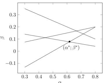
iii) Let ∆ and h fulfill

n∆h2 =T h2 → ∞and ∆1/2h−2 →0 as n → ∞.

Let us shortly remark that A2,i) and A2,ii) are standard in kernel based estimation procedures. One could also allow higher order kernels. A kernel function K is of order

l _∈N_{, if} Z R K(z)dz = 1, Z R zjK(z)dz = 0, j = 1, ..., l₋1 and Z R zlK(z)dz <_∞.

This would cause an asymptotic bias reduction, but the proofs are rather long and invoke tedious calculations. Further, such kernels lack the property of being a probability density anymore. These are reasons why we will only focus on kernels of order two. Certainly, all proofs can be carried over to more general kernels.

For our purposes, one can always think of the Gaussian kernel

KG(z) := √1

2πe

−12z2

as a toy-example for which all assumptions hold true. Of course, there are many other choices for kernel functions possible, but in the literature it is quite reputable that the choice of the kernel function is not as important as the choice of the bandwidth parameter. Later on, we will present an example for which assumption A2, iii) is fulfilled. In general, it turns out that ∆ has to converge relatively fast compared to h, which means that

(25)

2.4 Consistency of

ˆ

b

(

x

)

We are now ready to state our first theorem, namely the weak consistency of ˆb(x).

Theorem 2.6. Let assumptions A1 and A2 hold true. Then, provided that π(x)>0, we can conclude that

ˆ_b₍_x₎ P

−→b(x), as n_{→ ∞}.

We remark an essential difference to the findings in Bandi and Nguyen (2003) and to Mancini and Ren´o (2011): due to the possible occurrence of infinitely many jumps on a finite interval, we are only able to prove convergence in probability of our proposed estimator. The reason for this weaker result is relatively intuitive. It turns out that one of the key points of their proofs of the strong consistency is the uniform boundedness of increments ofX on small intervals. They defined for this purpose the value

δn,T := max

i≤n−1_i_∆_≤_ssup_≤₍_i_+1)∆|Xs−−Xi∆|.

Using L´evy´s modulus of continuity of the Brownian motion and due to the fact that only finitely many jumps occur on every small interval, they deduced that

lim supn→∞

δn,T

(∆ log(∆−1₎₎1/2 =C, a.s.

for some constant C; see Bandi and Nguyen (2003), equation (95).

We are not able to specify a comparable almost surely bound in our setting and, hence, will only deduce the convergence in probability of our proposed estimator.

Proof of Theorem 2.6. We will now derive the weak consistency of ˆb(x). For this

pur-pose we will divide the proof into different steps. At first, we decompur-pose ˆb(x) due to its definition: ˆ b(x) = 1 nh Pn−1 i=0 K Xi∆−x h (X(i+1)∆−Xi∆) ∆ nh Pn−1 i=0 K Xi∆−x h = 1 h Pn−1 i=0 K Xi∆−x h R(i+1)∆ i∆ b(Xs)ds+ R(i+1)∆ i∆ σ(Xs)dWs+ R(i+1)∆ i∆ ξ(Xs−)dLs ∆ h Pn−1 i=0 K Xi∆−x h := I+II+III IV .

(26)

Each term will be handled separately and we will start with the derivation of the denom-inator IV = ∆ h n−1 X i=0 K Xi∆−x h = Z T 0 1 hK x−Xs h ds+ ∆ h n−1 X i=0 K Xi∆−x h − Z T 0 1 hK x−Xs h ds = Z T 0 1 hK x₋Xs h ds+ 1 h n−1 X i=0 Z (i+1)∆ i∆ K Xi∆−x h −K x₋Xs h ds := Z T 0 1 hK x−Xs h ds+F₁n. (2.3)

We are interested in the rate of convergence of the approximation error Fn

1 and

con-sider therefore its L1_{-distance. Under the assumption that} _K _{is Lipschitz-continuous, by}

Proposition 2.3, the Cauchy-Schwarz as well as the Jensen inequality, we conclude that

E[|F₁n|]≤ 1 h n−1 X i=0 E "Z (i+1)∆ i∆ K Xi∆−x h −K x−Xs h ds # ≤ 1 h n−1 X i=0 E "Z (i+1)∆ i∆ || K′_||_∞ Xi∆−Xs h 1[i∆,(i+1)∆](s)ds # ≤ ||K′||∞ h2 n−1 X i=0 E   Z (i+1)∆ i∆ (Xi∆−Xs)2ds !1/2 ∆1/2 ≤ ∆ 1/2_||_K′_|| ∞ h2 n−1 X i=0 Z (i+1)∆ i∆ E[Xi∆−Xs)2] 1/2 ds . ∆ 1/2 h2 n−1 X i=0 Z (i+1)∆ i∆ ∆1/2ds= n∆ 2 h2 = T∆ h2 .

Using the Markov inequality, we can deduce that

P(|F₁n|> ε)≤ E[|F n 1|] ε =O(T∆h −2₎_{, ε >} ₀ ⇒F₁n =OP T∆ h2 , asn → ∞.

As we want to use the ergodic theorem for the first term of (2.3), we will multiply both terms by _T1. Definitely, we will do the same for the derivation of the numerator. AsT → ∞

(27)

and h→0 we conclude that 1 T ·IV = 1 T Z T 0 1 hK x₋Xs h ds+OP ∆ h2 −→π(x), as n, T _{→ ∞},

which means that

1

T ·IV

P

−→π(x), as n, T _{→ ∞}.

Now we will derive the three parts in the numerator of ˆb(x). We start with the drift term I: I = 1 h n−1 X i=0 K Xi∆−x h Z (i+1)∆ i∆ b(Xs)ds = Z T 0 1 hK x₋Xs h b(Xs)ds+ 1 h n−1 X i=0 Z (i+1)∆ i∆ K Xi∆−x h −K x₋Xs h b(Xs)ds := Z T 0 1 hK x−Xs h b(Xs)ds+F_bn. (2.4)

We again derive the L1_{-distance of the approximation error} _Fn

b . We will use comparable techniques as before, namely Proposition 2.3 and the Cauchy-Schwarz inequality. We will also rely on the fact that b(X0)∈L2(Γ(dx)) and conclude as follows:

E[_|Fn b |]≤ 1 h n−1 X i=0 Z (i+1)∆ i∆ EK Xi∆−x h −K x₋Xs h · |b(Xs)| ds ≤ 1 h n−1 X i=0 Z (i+1)∆ i∆ E " K Xi∆−x h −K x₋Xs h 2#!1/2 Eb2(Xs)1/2ds ≤ 1 h n−1 X i=0 Z (i+1)∆ i∆ E " ||K′||2 ∞ Xi∆−Xs h 2#!1/2 Eb2(Xs)1/2ds = (E[b 2₍_X 0)])1/2||K′||∞ h2 n−1 X i=0 Z (i+1)∆ i∆ E(Xi∆−Xs)2 1/2 ds . ∆ 1/2_T h2 .

We multiply again by T−1 _{and conclude that}

1 T ·F n b =OP ∆1/2 h2 .

(28)

Again, this term converges to zero due to A2, iii).

Finally, we receive for (2.4), as n and T diverge simultaneously, that 1

T ·I

P

−→b(x)π(x), as n, T → ∞,

where we used the standard substitution from above and recalled that b as well as π are continuous functions and that K(z)dz is a probability distribution.

Now we will handle term II:

II = 1 h n−1 X i=0 K Xi∆−x h Z (i+1)∆ i∆ σ(Xs)dWs.

We remark that this term is a martingale-difference sequence. Moreover, due to the sta-tionary and independent increments of the Brownian motionW, we are allowed to derive the L2_{-distance of this term in an easy manner. At first, remember that the probability}

space was endowed with a filtration of sub-σ-algebras _Ft =σ(X0,(Ws, Ls), s ≤t). With respect to this filtration, we can make use of conditional expectations to conclude that

E[II] =E[E[II_|Fi∆]] = E      1 h n−1 X i=0 K Xi∆−x h E "Z (i+1)∆ i∆ σ(Xs)dWs Fi∆ # | {z } =0     = 0.

Now, the variance can be decomposed into

E[II2] =E   1 h n−1 X i=0 K Xi∆−x h Z (i+1)∆ i∆ σ(Xs)dWs !2  = 1 h2 n−1 X i=0 E " K2 Xi∆−x h E "Z (i+1)∆ i∆ σ2₍_X s)ds Fi∆ ## + 1 h2E " _n₋₁ X i,j=0;i6=j K Xi∆−x h Z (i+1)∆ i∆ σ(Xs)dWs K Xj∆−x h Z (j+1)∆ j∆ σ(Xu)dWu # ≤σ1 ∆ h2 n−1 X i=0 E K2 Xi∆−x h + 2 h2E " X i<j K Xi∆−x h Z (i+1)∆ i∆ σ(Xs)dWs K Xj∆−x h Z (j+1)∆ j∆ σ(Xu)dWu # ≤ σ1n∆||K 2_|| ∞ h2 .

(29)

For the last step, we used the tower property of conditional expectations as follows: E " X i<j K Xi∆−x h Z (i+1)∆ i∆ σ(Xs)dWs K Xj∆−x h Z (j+1)∆ j∆ σ(Xu)dWu # =E X i<j K Xi∆−x h E Z (i+1)∆ i∆ σ(Xs)dWs K Xj∆−x h E "Z (j+1)∆ j∆ σ(Xu)dWu Fj∆ # | {z } =0 Fi∆ = 0.

Using Chebyshev´s inequality and assumption A2, ii) we are finally able to conclude that

P T−1_|II_|> ε_≤ E[II 2_] T2_ε2 =O T T2_h2 =O 1 T h2 =o(1), as n_{→ ∞} and therefore 1 T ·II =OP((T h 2₎−1/2_{) =}_o P(1), asn → ∞. Finally, the term

III = 1 h n−1 X i=0 K Xi∆−x h Z (i+1)∆ i∆ ξ(Xs−)dLs

can be handled in the exact same manner as the Brownian part. We assumed that L is anL2_{-martingale, which can be represented as an integral with respect to a compensated}

random measure. This is why term III is a martingale-difference sequence, too. Using the Burkholder-Davis-Gundy type inequality in Lemma 2.4 for L´evy driven stochastic integrals, we can derive the same asymptotic rate of convergence as for term II:

1

T ·III =OP((T h

2₎−1/2_{) =} _o

P(1), as n→ ∞.

Now we can summarize our recent findings and are able to complete the proof by the quotient limit theorem for stationary Markov processes; see Bandi and Nguyen (2003), p.

(30)

317: ˆ_b₍_x_{) =} T h1 Pn−1 i=0 K Xi∆−x h (X(i+1)∆−Xi∆) ∆ T h Pn−1 i=0 K Xi∆−x h = 1 T RT 0 1 hK Xs−x h b(Xs)ds+ _T1 _·Fn b +T1 ·II + 1 T ·III 1 T RT 0 1 hK Xs−x h ds+ 1 T ·F1n = 1 T RT 0 1 hK Xs−x h b(Xs)ds+OP ∆1/2 h2 +OP _{T h}12 1 T RT 0 1 hK Xs−x h ds+OP _h∆2 = b(x)π(x) +oP(1) π(x) +oP(1) =b(x) +oP(1), as n, T → ∞. Recall that we assumed that π(x)>0 holds true.

2.5 Derivation of the asymptotic distribution

From a practical point of view, it is desirable to be able to construct confidence inter-vals for estimated values of b(x). To derive our second important theorem, namely the asymptotic normality of ˆb(x), we have to strengthen our assumptions in a slightly different manner.

Assumption A3

i) Let the drift function b as well as the stationary density π be twice continuously differentiable.

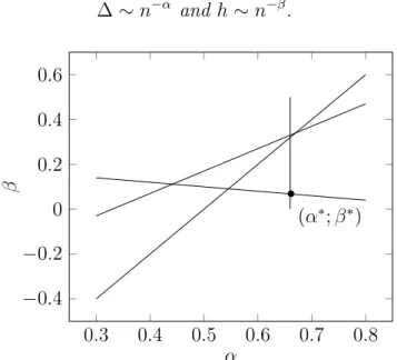
ii) Let ∆ andh satisfy

n∆h5 →0 andn∆2h−3 →0 as n→ ∞.

iii) Let the L´evy-measureν fulfill Z

R

y4ν(dy)<∞.

Now we are ready to state our next important theorem.

Theorem 2.7. Under Assumptions A1-A3, provided that π(x)>0, it holds that

√ n∆h(ˆb(x)₋b(x))_{−→ N}D 0,||K|| 2 2(V ar(L(1))ξ2(x) +σ2(x)) π(x) , as n_{→ ∞}.

(31)

We shortly remark that Assumption A3, ii) ensures that the bias term is negligible. It will turn out that the key point of the derivation of the asymptotic distribution will be a central limit theorem (CLT) for arrays of martingale-difference sequences. We will make use of the following version stated in Shiryayev, Probability (1995), page 511.

Theorem 2.8. Let (Yin,Fin)n∈N be a square-integrable array of martingale-difference

se-quences satisfying the Lindeberg condition: if for ε >0

⌊nt⌋ X i=0 E[Y2 i,n·1(|Yi,n|> ε)|Fi−1,n] P −→0 as n_{→ ∞} (2.5)

for a 0< t_≤1, it holds that

1.) ⌊(n_X−1)t⌋ i=0 E[Y2 i,n|Fi−1,n] P −→σ2 t =⇒ ⌊(n_X−1)t⌋ i=0 Yi,n→ ND (0, σ2t) 2.) ⌊(n_X−1)t⌋ i=0 Yi,n2 P −→σt2 =⇒ ⌊(n_X−1)t⌋ i=0 Yi,n→ ND (0, σ2t).

Another interesting result, stated below, will also be used and is concerned with moment properties of L´evy-driven stochastic integrals.

Lemma 2.9. Let X = (Xt)t_≥0 be the solution of (2.2) and let f be a bounded and

continuous function. Moreover, let Ξ = (Ξt)t_≥0 be a centered pure jump L´evy process

possessing the property that RRy

4_ν₍_dy₎ _< _∞_{. Define the process} _Y₍_t_{) =} Rt

0 f(Xs−)dΞs, then it holds that

i) E[Y2(t)] =E "Z t 0 f(Xs−)dΞs 2# = Z t 0 E[f2(Xs)]dsV ar(Ξ(1)) ii) E[Y4(t)] = 6 Z t 0 E[Y2(s)f2(Xs)]dsV ar(Ξ(1)) + 4 Z t 0 E[Y(s)f3₍_X s)]ds Z R y3_ν₍_dy_{) +} Z t 0 E[f4₍_X s)]ds Z R y4_ν₍_dy₎_.

For the derivation of this result we will need the Itˆo-formula for general semimartingales. We will state this fundamental result below, which can be found for instance in Protter (2005), Chapter 7, Theorem 32. We have already implicitly used it in the context of the approximation of the infinitesimal generator of the considered jump process X.

Theorem 2.10. Let X = (Xt)t_≥0 be a semimartingale and let g be a real valued C2

(32)

holds true: g(Xt)−g(X0) = Z (0,t] g′(Xs−)dXs+ 1 2 Z (0,t] g′′(Xs−)d[X, X]cs + X 0<s≤t (g(Xs)−g(Xs−)−g′(Xs−)∆Xs).

Proof of Lemma 2.9. Recall that Ξ is a martingale with respect to its augmented

canon-ical filtration.

Using the Itˆo-formula for semimartingales and especially choosingg(x) = x2_{, we are able}

to derive Y2₍_t_{) as} E[Y2(t)] =E Z t 0 Z R (Y(s₋) +y)2−Y2(s₋)−2Y(s₋)yν˜_sY(dy)ds +E Z t 0 Z R (Y(s₋) +y)2 −Y2(s₋)−2Y(s₋)y(˜µ_sY −ν˜_sY)(dy, ds) :=E Z t 0 Z R Y2(s₋) + 2Y(s₋)y+y2−Y2(s₋)−2Y(s₋)yν˜_sY)(dy)ds =E Z t 0 Z R y2ν˜_sY(dy)ds , where ˜µY

s(dy, ds) is the Poisson random measure corresponding to the process Y with its intensity measure ˜νY

s (dy)ds. Furthermore, ¯˜µYs(dy, ds) denotes the compensated random measure. Observe that the intensity measure is now time-dependent and that the second term is a martingale by construction. To derive a closed form of the time-dependent random measure, we make use of the following representation of ˜νY

s (A) ˜ ν_sY(A) = Z R 1A(f(Xs)x)ν(dx), _∀ A_{∈ B}(R₎_, ₀_∈_/ _A,

which can, for example, be found in Kallsen (2006), Proposition 2.4. Therefore, we can conclude that

E[Y2(t)] = E Z t 0 Z R y2ν˜_sY(dy)ds = Z t 0 Z R E[f2(Xs)]x2ν(dx)ds = Z t 0 E[f2(Xs)]dsE[L2(1)].

(33)

now by the use of g(x) = x4: Y4₍_t_{) =} Z t 0 Z R (Y(s₋) +y)4₋_Y4₍_s −)−4Y3(s−)y ˜ νY s (dy)ds + Z t 0 Z R (Y(s₋) +y)4−Y4(s₋)−4Y3(s₋)y(˜µ_sY −ν˜_sY)(dy, ds) = Z t 0 Z R 6Y2(s₋)y2+ 4Y(s₋)y3+y4ν˜_sY(dy)ds + Z R 6Y2₍_s −)y2+ 4Y(s−)y3+y4 _¯˜ µY s(dy, ds) = 6 Z t 0 Z R Y2(s₋)y2ν˜_sY(dy)ds+ 4 Z t 0 Z R Y(s₋)y3ν˜_sY(dy)ds + Z t 0 Z R y4ν˜_sY(dy)ds+Mt,

where Mt denotes the martingale part. Using analogous arguments, we are now able to deduce that E[Y4(t)] = 6 Z t 0 E[Y2(s)f2(Xs)]ds Z R y2ν(dy) + 4 Z t 0 E[Y(s)f3(Xs)]ds Z R y3ν(dy) + Z t 0 Z R E[f4(Xs)]ds Z R y4ν(dy) = 6 Z t 0 E[Y2(s)f2(Xs)]dsE[L2(1)] + 4 Z t 0 E[Y(s)f3(Xs)]ds Z R y3ν(dy) + Z t 0 Z R E[f4(Xs)]ds Z R y4ν(dy),

which finishes the proof.

An elementary consequence is the following upper bound

Corollary 2.11. Under the assumptions of Lemma 2.9, we can derive the following upper bounds E[Y2(t)]_{≤ ||}f_||2_∞V ar(L(1))t as well as E[Y4(t)]_≤3V ar2(L(1))_||f_||4_∞t2+8 p V ar(L(1))||f||4 ∞ 3 Z R y3ν(dy)t3/2+_||f_||4_∞ Z R x4ν(dx)t.

(34)

Proof of Corollary 2.11. We only state the proof of the second statement: E[Y(t)4] = 6 Z t 0 E[Y2(s)f2(Xs)]dsV ar(L(1)) + 4 Z t 0 E[Y(s)f3(Xs)]ds Z R y3ν(dy) + Z t 0 E[f4(Xs)]ds Z R y4ν(dy) ≤6_||f_||2_∞V ar(L(1)) Z t 0 E[Y2(s)]ds+ 4pV ar(L(1))_||f_||4_∞ Z R y3ν(dy) Z t 0 √ sds + Z t 0 E[f4(Xs)] Z R x4ν(dx) ≤6V ar2(L(1))||f||4 ∞ Z t 0 sds+ 8 p V ar(L(1))_||f_||4 ∞ 3 Z R y3ν(dy)t3/2 + Z t 0 E[f4(Xs)] Z R x4ν(dx) = 3V ar2(L(1))_||f_||4_∞t2+8 p V ar(L(1))||f||4 ∞ 3 Z R y3ν(dy)t3/2 + Z t 0 E[f4₍_X s)] Z R x4_ν₍_dx₎_.

Now we are able to state the proof of the asymptotic normality.

Proof of Theorem 2.7. We will start with a decomposition, comparable to derivation of

the consistency of ˆb(x): √ T h(ˆb(x)−b(x)) = √T h 1 T h Pn−1 i=0 K Xi∆h−x (X(i+1)∆−Xi∆) ∆ T h Pn−1 i=0 K Xi∆−x h −b(x) ! =√T h 1 T h Pn−1 i=0 K Xi∆−x h R(i+1)∆ i∆ (b(Xs)−b(x))ds ∆ T h Pn−1 i=0 K Xi∆h−x ! +√T h   1 T h Pn−1 i=0 K Xi∆−x h R(i+1)∆ i∆ σ(Xs)dWs+ R(i+1)∆ i∆ ξ(Xs−)dLs ∆ T h Pn−1 i=0 K Xi∆−x h   =√T h 1 T RT 0 1 hK x−Xs h (b(Xs)−b(x))ds+Fn b + T1F1n ∆ T h Pn−1 i=0 K Xi∆−x h ! (2.6) + 1 √ T h Pn−1 i=0 K Xi∆−x h R(i+1)∆ i∆ σ(Xs)dWs+ R(i+1)∆ i∆ ξ(Xs−)dLs ∆ T h Pn−1 i=0 K Xi∆−x h

(35)

The first term in (2.6) is a bias term and negligible as we will see in our subsequent analysis, because of T h5 ₌_n_∆_h5 _→_{0 as} _{n, T} _{→ ∞}_{. By the use of a Taylor expansion of}

the functionsb and π aroundx, we are able to handle the first term. Due to the fact that

b and π are twice continuously differentiable, the remainder terms are negligible and we can conclude that

Z R 1 hK x−y h (b(y)−b(x))π(y)dy = Z R K(z)(b(x−zh)−b(x))π(x−zh)dz = Z R K(z) −zhb′(x) + z 2_h2 2 b ′′₍_x_{) +}_O₍_h3₎ π(x)₋zhπ′(x) +O(h2)dz = Z K(z) b′(x)π(x)(−zh) +z2h2b′(x)π′(x)z 2_h2 2 b ′′₍_x₎_π₍_x₎ dz+O(h3) =h2 Z z2K(z)dz b′(x)π′(x) + b ′′₍_x₎_π₍_x₎ 2 +O(h3) = O(h2). (2.7) Now, by letting T → ∞, we can use the ergodic property of the process X and are able to derive the asymptotic rate of convergence of the numerator of (2.6) by the use of (2.7):

√ T h 1 T Z T 0 1 hK x₋Xs h (b(Xs)−b(x))ds+Fbn+ 1 TF n 1 =O((n∆h)1/2h2) +OP((n∆h)1/2∆1/2h−2) =oP(1), as n→ ∞. Where the last equality follows from A3, ii).

We already know that the denominator is a consistent estimate of π(x). Hence, we will now treat the remaining two terms of the numerator, which we define as

n−1 X i=0 ηi+1,n := 1 √ T h n−1 X i=0 K Xi∆−x h Z (i+1)∆ i∆ σ(Xs)dWs = n−1 X i=0 ˜ ηi+1,n+FWn as well as n−1 X i=0 ζi+1,n := 1 √ T h n−1 X i=0 K Xi∆−x h Z (i+1)∆ i∆ ξ(Xs−)dLs := n−1 X i=0 ˜ ζi+1,n+FnL, where F_nL = √1 T h n−1 X i=0 Z (i+1)∆ i∆ ξ(Xs−) K x−Xs− h −K x−Xi∆ h dLs and F_nW = √1 T h n−1 X i=0 Z (i+1)∆ i∆ σ(Xs) K x−Xs h −K x−Xi∆ h dWs

(36)

are denoting the approximation errors. Both terms are negligible in probability, which can be seen through E[(F_nL)2] = 1 T h n−1 X i=0 Z (i+1)∆ i∆ E " ξ2(Xs) K x₋Xs h −K x₋Xi∆ h 2# V ar(L(1))ds ≤ ||K′|| 2 ∞||ξ2||∞V ar(L(1)) T h3 n−1 X i=0 Z (i+1)∆ i∆ E(Xi∆−Xs)2 ds . n∆ 2 T h3 = ∆ h3 =o(1), asn → ∞,

where the last equation follows from the fact that ∆1/2_h−2 _→ _{0. Therefore, this term is}

negligible in probability by the fact that FL

n = OP(∆1/2h−3/2) = oP(1) as n, T → ∞. This suffices, because we are interested in convergence in distribution. We only used the fact that L is a process with stationary and independent increments such that the L´evy measureν(dy) integrates y4 _{to a finite number. Therefore, the order of} _FW

n can be found in a similar manner.

Now we will focus on the array of martingale difference sequences (˜ηi+1,n,Fi) and (˜ζi+1,n,Fi). Both can be treated by the use of central limit theorem 2.8. Recall that we chose Ft =

σ(X0,(Ws, Ls);s ≤ t) as filtration. We will start with the verification of the Lindeberg condition (2.5) for t= 1 by the following useful observation:

n−1 X i=0 E[˜ζ_i2₊₁_,n1(_|ζ˜i+1,n|> ε)|Fi∆] = n−1 X i=0 Z R y21(_|y_|> ε)Pζ˜i+1,n|Fi∆₍_dy₎ ≤ n−1 X i=0 Z R y4 ε21(|y|> ε)P ˜ ζi+1,n|Fi∆₍_dy₎_≤ n−1 X i=0 Z R y4 ε2P ˜ ζi+1,n|Fi∆₍_dy₎ = 1 ε2 n−1 X i=0 E[˜ζ_i4₊₁_,n_|Fi∆].

Now recall the statement of Lemma 2.4. This lemma enables us to derive upper bounds for moments of L´evy as well as Brownian driven stochastic integrals. Instead of the function

ξ, we will now make use of the lemma by the utilization of the function ˜ξ:=K_·ξ, which is again bounded and also continuous. For the determination of the fourth conditional moment of ˜ζi+1,n we need the statement of Lemma 2.4 in a slightly more general form. By Schmisser (2014), p.895, it holds, because RRy

4_ν₍_dy₎_<_∞_{, that} E "Z t+∆ t K x₋Xu h σ(Xu)dWu 4 Fi∆ # ≤E " sup |t−s|≤∆ Z s t K x−Xu h σ(Xu)dWu 4 Fi∆ #

(37)

≤C˜1E "Z t+∆ t K2 x−Xu h σ2(Xu)du 2 Fi∆ # ≤C˜1||K2σ2||2_∞∆2.

For the L´evy driven integral we find analogously

E "Z t+∆ t K x₋Xu− h ξ(Xu−)dLu 4 Fi∆ # ≤E " sup |t−s|≤∆ Z s t K x−Xu− h ξ(Xu−)dLu 4 Fi∆ # ≤C˜2(V ar(L(1)))2E "Z t+∆ t K2 x₋Xu h ξ2(Xu)du 2 Fi∆ # + ˜C2 Z R y4ν(dy)E Z t+∆ t K4 x₋Xu h ξ4(Xu)du Fi∆ ≤C˜2 (V ar(L(1)))2_||K2σ2_||2_∞∆2+ Z R y4ν(dy)_||K4ξ4_||_∞∆ ,

where ˜C2 denotes a deterministic constant.

We shortly remark that both integrands are non-negative and bounded functions such that the result of Schmisser (2014), p.895, can be transferred. These inequalities can also be found in Dellacherie and Meyer (1980), Theorem 92, Chapter VIII and Applebaum (2004), Theorem 4.4.23, p. 265.

Now we are able to verify the Lindeberg condition: n−1 X i=0 E[˜ζ2 i+1,n1(|ζ˜i+1,n|> ε)|Fi∆]≤ 1 ε2 n−1 X i=0 E[˜ζ4 i+1,n|Fi∆] = 1 ε2 n−1 X i=0 E   _√1 T h Z (i+1)∆ i∆ K _x −Xs− h ξ(Xs−)dLs !4 Fi∆   ≤ 1 T2_h2_ε2 n−1 X i=0 ˜ C2 (V ar(L(1)))2_||K2σ2_||2_∞∆2+ Z R y4ν(dy)_||K4ξ4_||_∞∆ . n∆ 2 T2_h2 + n∆ T2_h2 =O 1 nh2 +O 1 T2_h2 =o(1), as n, T _{→ ∞}.

(38)

of the second condition of central limit theorem 2.8: n−1 X i=0 E[˜ζi2+1,n|Fi∆] = n−1 X i=0 E   _√1 T h Z (i+1)∆ i∆ K _x −Xs− h ξ(Xs−)dLs !2 Fi∆   := 1 T h n−1 X i=0 E(ζ(′i+1)∆−ζi′∆)2|Fi∆ = 1 T h n−1 X i=0 E(ζ₍′_i_+1)∆)2₋(ζ_i′_∆)2_|Fi∆−2E[ζi′∆(ζ(′i+1)∆−ζi′∆)|Fi∆] = 1 T h n−1 X i=0 E(ζ₍′_i_+1)∆)2₋(ζ_i′_∆)2_|Fi∆ −2ζ_i′_∆E[ζ₍′_i_+1)∆₋ζ_i′_∆_|Fi∆] = 1 T h n−1 X i=0 E(ζ₍′_i_+1)∆)2−(ζ_i′_∆)2|Fi∆ = 1 ∆h 2 n n X i=1 Z (i+1)∆ i∆ E ζ_s′₋dζ_s′ Fi∆ + 1 ∆h 1 n n X i=1 Z (i+1)∆ i∆ E K2 x₋Xs− h ξ2(Xs−)y 2_µ_¯₍_{ds, dy}₎ Fi∆ + 1 ∆h 1 n n X i=1 Z (i+1)∆ i∆ E K2 x₋Xs h ξ2₍_X s) Fi∆ ds Z R y2_ν₍_dy₎_.

By using the ergodicity of X we see that the first two terms converge to zero due to the fact that they are martingales. The third summand converges by invoking the stationarity of X to

V ar(L(1))ξ2(x)π(x) Z

R

K2(z)dz, asn, T → ∞.

According to central limit theorem 2.8, this value denotes the asymptotic variance of this part.

Now we have almost finished the proof of the asymptotic normality. For the L´evy driven part, we are now able to summarize that

√ T h_{T h}1 Pn_i₌₀−1K x−Xi∆ h R(i+1)∆ i∆ ξ(Xs−)dLs ∆ T h Pn−1 i=0 K x−Xi∆ h 1 √ T h Pn−1 i=0 K x−Xi∆ h R(i+1)∆ i∆ ξ(Xs−)dLs π(x) +OP _h∆2