Projection methods for clustering and semi-supervised classification

Clustering and

Semi-supervised

Classification

David Paul Hofmeyr, B.Sc. (Hons), M.Sc., M.Res.

Submitted for the degree of Doctor of Philosophy at Lancaster University

This thesis focuses on data projection methods for the purposes of cluster-ing and semi-supervised classification, with a primary focus on clustercluster-ing. A number of contributions are presented which address this problem in a principled manner; using projection pursuit formulations to identify sub-spaces which contain useful information for the clustering task. Projection methods are extremely useful in high dimensional applications, and situa-tions in which the data contain irrelevant dimensions which can be counter-informative for the clustering task. The final contribution addresses high dimensionality in the context of a data stream. Data streams and high dimen-sionality have been identified as two of the key challenges in data clustering. The first piece of work is motivated by identifying the minimum density hyperplane separator in the finite sample setting. This objective is directly related to the problem of discovering clusters defined as connected regions of high data density, which is a widely adopted definition in non-parametric statistics and machine learning. A thorough investigation into the theoretical aspects of this method, as well as the practical task of solving the associated optimisation problem efficiently is presented. The proposed methodology is applied to both clustering and semi-supervised classification problems, and is shown to reliably find low density hyperplane separators in both contexts. The second and third contributions focus on a different approach to clus-tering based on graph cuts. The minimum normalised graph cut objective has gained considerable attention as relaxations of the objective have been devel-oped, which make them solvable for reasonably well sized problems. This has been adopted by the highly popular spectral clustering methods. The second piece of work focuses on identifying the optimal subspace in which to perform spectral clustering, by minimising the second eigenvalue of the graph Laplacian for a graph defined over the data within that subspace. A rigorous treatment of this objective is presented, and an algorithm is pro-posed for its optimisation. An approximation method is propro-posed which allows this method to be applied to much larger problems than would other-wise be possible. An extension of this work deals with the spectral projection pursuit method for semi-supervised classification.

cut to be computed, rather than the spectral relaxation. It also allows for a computationally efficient method for optimisation. The asymptotic properties of the normalised cut based on a hyperplane separator are investigated, and shown to have similarities with the clustering objective based on low den-sity separation. In fact, both the methods in the second and third works are shown to be connected with the first, in that all three have the same solution asymptotically, as their relative scaling parameters are reduced to zero.

The final body of work addresses both problems of high dimensionality and incremental clustering in a data stream context. A principled statistical framework is adopted, in which clustering by low density separation again becomes the focal objective. A divisive hierarchical clustering model is pro-posed, using a collection of low density hyperplanes. The adopted frame-work provides well founded methodology for determining the number of clusters automatically, and also identifying changes in the data stream which are relevant to the clustering objective. It is apparent that no existing methods can make both of these claims.

To begin with I would like to thank my supervisors. Nicos, your enthusi-asm for the work we have done during my thesis has been a great source of motivation. Idris, you have always provided an encouraging and somehow calming perspective on my research, and research in general. I have learned a lot from both of you, and I am extremely grateful. Thanks too for putting up with me these past few years, I know that my repeatedly ignoring your advice and comments can’t always have gone unnoticed.

I would also like to thank both the EPSRC and the Oppenheimer Memo-rial Trust for providing funding during my Ph.D.

To Jon, Idris and Kevin; the STOR-i doctoral training centre has been the ideal environment in which to do my Ph.D. You’ve outdone yourselves. Thank you.

To the friends I have made during my time here in Lancaster, in particu-lar my year group in STOR-i, you’ve always provided sufficient distractions from work to make the Ph.D seem manageable, even when things have been difficult. The whole process could not have been nearly as enjoyable without you guys.

To my family, you have been continuous sources of support and encour-agement and I will forever be grateful. The admittedly too infrequent chats, though perhaps seemingly just chats, have sometimes felt like the only thing keeping me going.

Finally, to Aeysha, your love and encouragement has been constant and I don’t know if I could have managed without that. There are a lot of things I could say, but I think what captures it well (at least it does for me), is that you stubbornly refuse to ever accept that I could have shortcomings; you always manage to find some other explanation for why I could be struggling. Thank you, for your oblivion, for everything.

I declare that the work in this thesis has been done by myself and has not been submitted elsewhere for the award of any other degree.

Abstract iii

Acknowledgements v

Declaration vii

Thesis Details xiii

List of Figures xiii

List of Tables xvii

1 Introduction 1

1 Clustering . . . 4

1.1 Centroid-Based Clustering . . . 5

1.2 Connectivity-Based Clustering . . . 6

1.3 Graph Partitioning Based Clustering . . . 8

1.4 Density-Based Clustering . . . 10

1.5 Model-Based Clustering . . . 11

2 Semi-supervised Classification . . . 12

2.1 Low Density Separation Methods . . . 13

2.2 Graph Partition Based Methods . . . 14

3 Challenges in Data Clustering . . . 15

3.1 High Dimensionality . . . 15

3.2 Data Streams . . . 17

4 Focus of Thesis . . . 19

4.1 Contributions . . . 19

2 Minimum Density Hyperplane: An Unsupervised and Semi-supervised Classifier 21 1 Introduction . . . 22

2 Problem Formulation . . . 25

2.2 Semi-Supervised Classification . . . 30

3 Connection to Maximum Margin Hyperplanes . . . 31

3.1 MDP2for Clustering . . . 34

3.2 MDP2for Semi-Supervised Classification . . . 35

4 Estimation of Minimum Hyperplanes . . . 36

4.1 Computational Complexity . . . 38

5 Experimental Results . . . 38

5.1 Clustering . . . 39

5.2 Semi-Supervised Classification . . . 45

5.3 Summary of Experimental Results . . . 48

6 Conclusions . . . 49

Appendix. Proof of Theorem 1 . . . 50

7 Proof of Theorem 1 . . . 50

3 Projection Pursuit Based on Spectral Connectivity 54 A. Minimum Spectral Connectivity Projection Pursuit for Unsuper-vised Classification 55 1 Introduction . . . 55

2 Related Work . . . 58

3 Background on Spectral Clustering. . . 59

4 Projection Pursuit for Spectral Connectivity. . . 61

4.1 Continuity and Differentiability . . . 62

4.2 Minimisingλ2(L(θθθ))andλ2(Lnorm(θθθ)). . . 67

4.3 Computing Similarities . . . 69

4.4 Correlated and Orthogonal Projections . . . 71

5 Connection with Maximal Margin Hyperplanes . . . 74

6 Speeding up Computation using Microclusters. . . 79

7 Experimental Results . . . 86

7.1 Details of Implementation. . . 87

7.2 Clustering Results . . . 89

7.3 Summarising Clustering Performance . . . 93

7.4 Sensitivity Analysis . . . 95

8 Conclusions . . . 98

Appendix. Derivatives . . . 100

B. Semi-supervised Spectral Connectivity Projection Pursuit 103 1 Introduction . . . 103 2 Spectral Clustering . . . 105 3 Methodology . . . 105 3.1 Computational Complexity . . . 110 4 Experiments . . . 111 5 Conclusions . . . 112

Appendix. Proofs . . . 114

4 Clustering by Minimum Cut Hyperplanes 118 1 Introduction . . . 118

2 Problem Formulation . . . 120

2.1 Background on Normalised Graph Cuts . . . 121

2.2 Normalised Cuts Across Hyperplanes. . . 121

2.3 Connection with Maximum Margin Hyperplanes . . . . 126

3 Methodology . . . 128

3.1 Optimal NCut of the Marginal Data Setv· X . . . 128

3.2 OptimisingΦ(v|X) . . . 130

3.3 Beyond Bi-partitioning. . . 133

4 Experimental Results . . . 134

4.1 Parameter Settings for NCutH and NCutH0 . . . 135

4.2 Clustering Performance . . . 136

4.3 Run Time Analysis . . . 138

5 Conclusion . . . 141

Appendix. Proofs . . . 142

5 Divisive Clustering of High Dimensional Data Streams 150 1 Introduction . . . 150

2 Related Work . . . 153

3 Problem Description . . . 154

4 Methodology . . . 157

4.1 Learning High Variance Projections . . . 157

4.2 Splitting Based on a Projected Sample . . . 158

4.3 Handling Population Drift . . . 164

5 The HSDC Algorithm . . . 166

5.1 Computational Complexity . . . 167

6 Experimental Results . . . 168

6.1 Simulations . . . 170

6.2 Publicly Available Data Sets . . . 175

6.3 Discussion of Experimental Results . . . 178

7 Conclusion . . . 179

Appendix. Proofs . . . 180

6 Conclusion 184 1 Summary of Contributions . . . 184

2 An Experimental Comparison of the Contributions . . . 187

2.1 Projected Divisive Clustering . . . 187

2.2 Large Margin Clustering . . . 188

2.3 A Summary of Clustering Performance . . . 189

3 Possible Extensions and Future Work . . . 195

Bibliography 197

Thesis Title: Projection Methods for Clustering and Semi-supervised Classification

Ph.D. Student: David Paul Hofmeyr

Supervisors: Dr. Nicos Pavlidis, Lancaster University Prof. Idris Eckley, Lancaster University Examiners: Dr. Ludger Evers, University of Glasgow

Dr. Chris Sherlock, Lancaster University The main body of this thesis consist of the following papers.

• Chapter2has been submitted for publication as; Pavlidis, N. G., Hofmeyr, D. P and Tasoulis, S. K. “Minimum Density Hyperplanes,” 2016.

• Chapter 3 A. has been submitted for publication as; Hofmeyr, D. P, Pavlidis, N. G. and Eckley, I. “Minimum Spectral Connectivity Projec-tion Pursuit for Unsupervised ClassificaProjec-tion," 2016.

• Chapter3 B. has been accepted for publication as; Hofmeyr, D. P. and Pavlidis, N. G. “Semi-supervised Spectral Connectivity Projection Pur-suit",PRASA-RobMech International Conference, 2015.

• Chapter4has been submitted for publication as; Hofmeyr, D. P. “Clus-tering by Minimum Cut Hyperplanes", 2016.

• Chapter5has been accepted for publication as; Hofmeyr, D. P., Pavlidis, N. G. and Eckley, I. “Divisive Clustering of High Dimensional Data Streams,"Statistics and Computing, issn: 0960-3174, doi: 10.1007/s11222-015-9597-y, Springer, 2015.

The majority of works involved collaboration with others, most notably my supervisors. In the case of Chapter2, Nicos Pavlidis took an especially sig-nificant role.

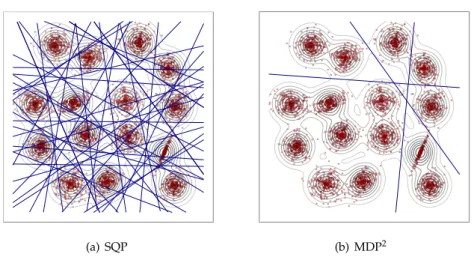
2.1 Binary partitions induced by 100 MDHs estimated through SQP and MDP2 . . . 29

2.2 Impact of choice ofαon minimum density hyperplane. . . 42

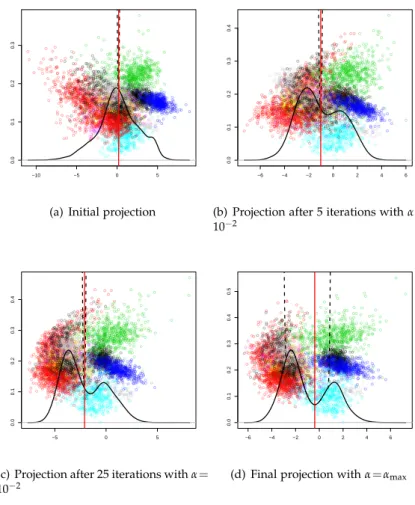
2.3 Evolution of the minimum density hyperplane through con-secutive iterations. . . 43

2.4 Performance and Regret Distributions for all Methods Consid-ered . . . 46

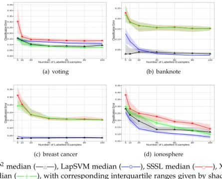
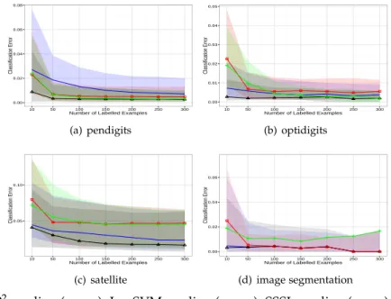
2.5 Classification error for different number of labelled examples for datasets with two clusters.. . . 47

2.6 Classification error for different numbers of labelled examples over all pairwise combinations of classes. . . 48

2.7 Two dimensional illustration of Lemma 8 . . . 51

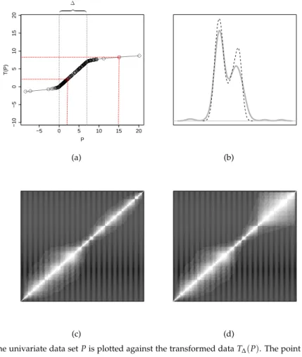
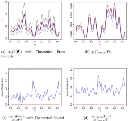
3.1 Effect ofT_∆on Distances and Similarities.. . . 72

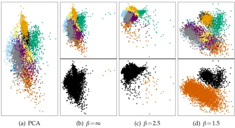
3.2 Two dimensional projections of optical recognition of hand-written digits dataset arising from the minimisation ofλ2(L(θθθ)),

for different values ofβ. In addition, the initialisation through

PCA is also shown. The top row of plots shows the true clus-ters, while the bottom row shows resulting bi-partitions. . . . 73

3.3 Large Euclidean separation of the yeast cell cycle dataset. The left plots show the result from a 2 dimensional projection pur-suit using the proposed method. The middle plots show the 1 dimensional projection pursuit result. The right plots show the result of the maximum margin clustering method of Zhang et al. (2009). . . 79

3.4 Approximation Error Plots for S1 data set. . . 85

3.5 Box plots of relative purity with additional red dots to indicate means. Methods are ordered with decreasing mean value. . . 96

3.6 Box plots of relative V-measure with additional red dots to indicate means. Methods are ordered with decreasing mean value. . . 97

3.7 Sensitivity analysis for varying σ. Standard Laplacian. The x-axis contains the multiplication factor applied to the default

scaling parameter used in the experiments. . . 97

3.8 Sensitivity analysis for varyingσ. Normalised Laplacian. The x-axis contains the multiplication factor applied to the default scaling parameter used in the experiments. . . 98

3.9 Sensitivity analysis for varying number of microclusters, K. Plots show median and interquartile ranges of performance measures from 30 datasets simulated from 50 dimensional Gaus-sian mixtures with 5 clusters and 1000 observations. . . 99

3.10 Sensitivity analysis for fixed number of microclusters, K = 200, and varying number of data. Plots show median and in-terquartile ranges of performance measures from datasets sim-ulated from 50 dimensional Gaussian mixtures with 5 clusters and between 1000 and 10 000 observations. . . 100

3.11 Two projections, one admitting a separation of the classes (Left) and the other not (Right). . . 109

4.1 Optimal hyperplanes based on NCut (left) and RatioCut (right) from the same 100 initialisations . . . 126

4.2 Regret distributions of Purity (top) and V-Measure (bottom) across all 15 benchmark data sets. . . 140

4.3 Run time analysis from Gaussian mixtures. The plot shows the medians and interquartile ranges from 50 replications for each value ofn. The number of clusters is fixed at 5. . . 140

5.1 Different changes in distribution and their impact on the clus-tering model. Red lines indicate necessity of model revision. Green lines indicate changes which can be addressed by ex-tending the model without revision . . . 165

5.2 Performance on Static Data Stream with 20 Classes in 500 Di-mensions . . . 171

5.3 Clustering Performance. Static Environment with Irrelevant Features. 20 Classes in 100 Relevant and 100 Irrelevant Dimen-sions with Moderate Variability . . . 172

5.4 Clustering Performance. Decreasing Classes. 500 Dimensions . 174 5.5 Clustering Performance. Increasing Classes. 500 Dimensions . 175 5.6 Clustering Performance. Distribution Overhaul. 20 Classes in 500 Dimensions . . . 176

5.7 Class Proportions of Forest Cover Type . . . 177

5.8 Clustering Performance. Forest Cover Type Data. . . 177

6.1 Box plots of relative purity with additional red dots to indicate means. Methods are ordered with decreasing mean value. . . 192

6.2 Box plots of relative V-measure with additional red dots to indicate means. Methods are ordered with decreasing mean value. . . 193

6.3 Box plots of regret based on purity with additional red dots to indicate means. Methods are ordered with increasing mean value. . . 194

6.4 Box plots of regret based on V-measure with additional red dots to indicate means. Methods are ordered with increasing mean value. . . 195

2.1 Details of Benchmark Data Sets . . . 39

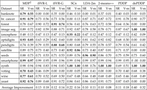
2.2 Performance on the task of binary partitioning. (Ties in best performance were resolved by considering more decimal places) 45

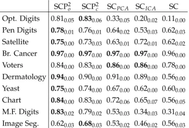
3.1 Purity results for spectral clustering using the standard Lapla-cian, L. Average performance from 30 runs on each dataset, with standard deviation as subscript. The highest average per-formance in each case is highlighted in bold. . . 90

3.2 V-measure results for spectral clustering using the standard Laplacian,L. Average performance from 30 runs on each dataset, with standard deviation as subscript. The highest average per-formance in each case is highlighted in bold. . . 91

3.3 Purity results for spectral clustering using the normalised Lapla-cian,Lnorm. Average performance from 30 runs on each dataset,

with standard deviation as subscript. The highest average per-formance in each case is highlighted in bold. . . 92

3.4 V-measure results for spectral clustering using the normalised Laplacian, Lnorm. Average performance from 30 runs on each

dataset, with standard deviation as subscript. The highest av-erage performance in each case is highlighted in bold. . . 92

3.5 Purity results for large margin clustering. Average perfor-mance from 30 runs on each dataset, with standard deviation as subscript. The highest average performance in each case is highlighted in bold. . . 93

3.6 V-measure results for large margin clustering. Average perfor-mance from 30 runs on each dataset, with standard deviation as subscript. The highest average performance in each case is highlighted in bold. . . 94

3.7 UCIMLR Classification Data Sets. Average Accuracy (%) over 10 Splits. . . 113

4.1 Details of Benchmark Data Sets . . . 135

4.2 100 × Purity on Benchmark Data Sets. Highest Performance Highlighted in Bold. . . 138

4.3 100 × V-Measure on Benchmark Data Sets. Highest Perfor-mance Highlighted in Bold. . . 139

4.4 Run Time on Benchmark Data Sets (in Seconds) . . . 141

5.1 Clustering Performance. Static environments. . . 171

5.2 Clustering Performance. Static environments with irrelevant features. . . 173

5.3 Clustering Performance. Drifting environments. . . 176

6.1 A Comparison of the Performance of Proposed Methods for Projected Divisive Clustering. The Table Shows 100× Purity on Benchmark Data Sets. Highest Performance in Each Case is Highlighted in Bold. . . 188

6.2 A Comparison of the Performance of Proposed Methods for Large Margin Clustering. The Table Shows 100 × V-Measure on Benchmark Data Sets. Highest Performance in Each Case is Highlighted in Bold. . . 189

6.3 A Comparison of the Performance of Proposed Methods for Large Margin Clustering. The Table Shows 100 × Purity on Benchmark Data Sets. Highest Performance in Each Case is Highlighted in Bold. . . 190

6.4 A Comparison of the Performance of Proposed Methods for Large Margin Clustering. The Table Shows 100 × V-Measure on Benchmark Data Sets. Highest Performance in Each Case is Highlighted in Bold. . . 191

6.5 A Comparison of the Proposed Methods for Semi-supervised Classification applied to UCI Machine Learning Repository Clas-sification Data Sets. Average Accuracy (%) over 10 Splits.. . . . 193

6.6 A Comparison of the Proposed Methods for Semi-supervised Classification applied to Benchmark Data Sets taken from Chap-elle et al. (2006b). Average Accuracy (%) over 12 Splits. . . 194

Introduction

The problem of identifying groups of related objects is one of the fundamen-tal tasks in knowledge discovery from data. This problem has been exten-sively studied in the literature on statistics, machine learning, data mining and pattern recognition because of the numerous applications in summarisa-tion, learning and segmentation (Jain and Dubes,1988;Aggarwal and Reddy,

2013). Such applications include,

• Engineering: In manufacturing, group technology seeks to identify sim-ilar items so that manufacturing and design concepts can be borrowed, thus speeding up the manufacturing lifecycle of emerging items (Pham and Afify, 2007). In radar signal analysis, the direction of arrival of pulses is crucial for object locating, however the sheer density of sig-nals creates a computational challenge which is mitigated by identi-fying groups of pulses (Zhu et al.,2010). Outlier rejection deals with separating a single group of objects from remaining nuisance observa-tions which do not fit within the group’s context, this has applicaobserva-tions in robotics in the form of consistent hypothesis identification (Olson et al.,2005).

• Computer Science: Web mining deals with organising the billions of web pages on the internet, so that queries can be handled efficiently. Grouping similar web objects, often by textual content, significantly aids this challenging task (Chen and Chau,2004). Computer vision and image segmentation tasks require identifying different planar ranges in an image, which may be achieved by grouping small sections of an image, or sequence of images, to determine separate planes and using their respective orientation and geometry (Frigui and Krishnapuram,

1999).

geo-graphical ancestries can be aided by finding similar allele groups from spatially recorded genetic information (Rosenberg et al.,2002). Group-ing lifestyle factors which have higher combined prevalence in indi-viduals suffering certain diseases than would be predicted given their individual prevalence has use in preventative medicine (Schuit et al.,

2002).

• Social Sciences: Person perception, in the field of psychology, looks at the different mental processes used to form impressions of peo-ple. Grouping people based on their perceptions of archetypal life fig-ures has been useful in identifying psychopathologies (Rosenberg et al.,

1996). The success of an education institution is predicated on both aca-demic performance and enrollment management. Grouping students based on their persistence with academic courses can be useful in both areas, especially for early identification of potential defectors (Luan,

2002).

• Commerce: Market segmentation can be achieved by identifying groups of related consumers or products (Punj and Stewart,1983), and is a cen-tral feature in targeted marketing strategy. Outlier rejection, as in the robotics application, can also be used to identify fraudulent behaviour of consumers or organisations, comparing behavioural patterns with the general behaviour of a group (Phua et al.,2010).

Broadly speaking the task of assigning a set of objects to groups may be termedclassification(Jain and Dubes,1988), and exists on three distinct levels in terms of the assumed available information. In the machine learning lit-erature the amount of information available may be described by degrees of

supervisionfor the learning task. On one end of the spectrum is the fully

su-pervised classification task, in which the true groupings of all data used in the learning phase of the task are known. An inductive model is then built which can be used to predict the groupings of future data. It is the fully supervised task which is commonly given the name “classification". On the other end of the spectrum lies unsupervised classification. In this context there is no ex-plicit information regarding how data should be grouped. The relationships between data must therefore be learned by other means. In this context any model which assigns groupings to data is used only within the context of the data used to build the model, and is not used to predict the groupings of future unseen data. Between these extremes lies semi-supervised classifica-tion. The motivation for semi-supervised classification can be seen as follows. When using a (supervised) classification model to predict the groupings of new data, there is an implicit assumption that the nature of those new data, in terms of their grouping tendencies, is somewhat related to the nature of the data used in building the model. If this assumption is true, then

utilis-long. Semi-supervised classification is extremely useful in situations where identifying the true grouplabelsfor data is expensive. In such situations the number of labelled data may be small, and making inference or prediction from a (supervised) classification model can be unreliable, and the prediction task can be substantially aided by utilising every bit of available information. This thesis focuses on the latter two, with a primary focus on the unsu-pervised problem. Semi-suunsu-pervised classification is treated within the same framework, as an extension of the unsupervised case. Utilising information about data which does not explicitly determine their groups is therefore the central feature of the work presented. Throughout the remainder it is as-sumed that a data set is described by a fixed set of features, each taking a (real) numerical value. Data may therefore be thought of as occupying a vec-tor space defined over the real numbers in which the number of dimensions is equal to the number of features describing the data.

A common assumption when data arise from multiple groups, or classes, is that the data tend to contain multiple clusters, and that objects within the same cluster are more likely to represent the same group. In the con-text of semi-supervised classification this is referred to as thecluster assump-tion(Chapelle and Zien,2005), and in the unsupervised case leads to the field of cluster analysis. Cluster analysis has a very rich history, and remains one of the most active and important areas of research in fields relying on the analysis of data. The term cluster analysis, or simplyclustering, is often used to refer to the task of unsupervised classification.

Accepting the cluster assumption immediately begs the question of what constitutes a cluster of data, and numerous definitions have been proposed, each leading to hosts of methods for identifying clusters which adhere to these definitions. Arguably the single common concept underpinning all of these, though, is that the spatial relationships between data contain useful information for determining clusters. The spatial relationships in this con-text are defined by the topological structure bestowed on the vector space containing the data, usually via the Euclidean (or L2) norm, although other

metrics may be used.

This thesis is motivated by two of the key challenges associated with data clustering, both from practical and theoretical points of view. The principal motivation comes from the problem of dimension reduction. Dimension re-duction forms a crucial part of the analysis of data which are either high dimensional, i.e., data containing a very large number of features, or data which contain features, or combinations of features, that may be irrelevant or even counter-informative for identifying clusters. A number of

contri-butions are presented which address this problem in a principled manner; using projection-pursuit formulations to identify subspaces which contain useful information for the clustering task. A secondary motivation arises from the challenge associated with clustering data incrementally, where data are received sequentially in a data stream. The final contribution of this thesis addresses both challenges, and proposes a method for clustering high dimen-sional data streams within a principled statistical framework. Further details of these contributions are given at the end of this chapter.

The remainder of this chapter is organised as follows. In Section1a number of cluster definitions are explored, as well as some important methods for finding clusters which fit within their respective definitions. In Section 2 a discussion of semi-supervised classification methods will be presented, with particular attention to those adhering to the cluster assumption. Following that, in Section 3 some fundamental challenges associated with clustering methods from practical, theoretical and philosophical perspectives will be presented. The focus of the remaining thesis will then be outlined in Sec-tion4.

Neither of Sections1and2is intended to be a comprehensive account of the entire literature on these problems, but rather provides a representative cross section of concepts and methods which are either highly influential or of relevance in the remaining thesis. Each subsequent chapter will contain its own review, documenting existing approaches which are of particular importance for the context of that chapter.

1

Clustering

This section is dedicated to the discussion of existing methods for clustering. Important concepts and methods in the clustering literature are discussed un-der the headings relating to different definitions of what constitutes a clus-ter. Clustering methods can also be split between two distinct approaches to model structure. Hierarchical clustering models are nested sequences of partitions (Jain and Dubes,1988) and may be further categorised into divi-sive and agglomerative clustering. In dividivi-sive clustering, beginning with the entire data set being a cluster, clusters are recursively partitioned until a stop-ping criterion is met. Conversely, agglomerative clustering begins with every datum in its own cluster, and repeatedly merges clusters until all data are contained in a single cluster. Partitional clustering models instead directly assign data to their final clusters in a single step. Partitional methods may also be referred to as generating aflat clustering. The focus of this section will be more strongly motivated by the concept of what constitutes a cluster, than by the model structure in which the clusters reside. The reason being that

the philosophy behind a particular approach to establishing or identifying re-lated groups of objects is much more closely rere-lated to the group definitions than their representation.

1.1

Centroid-Based Clustering

Centroid-based clustering defines clusters in relation to single representative points (centroids). Data are thought to collect around these points, forming clusters. Models derived from these clustering methods may be summarised by a set of centroids, and data are classified based on which centroid is near-est to them (Leisch,2006). This approach generates a partitional clustering model.

Formally, the clustering task may be stated in relation to the following optimisation problem, min C∈Fk n

∑

Here the xi,i = 1, ...,n represent the data points and the set C is the set

of centroids over which the optimisation takes place. The set F represents the collection of feasible centroid values. The function f : R+ → R+ _is non-decreasing, and operates on the distances between the data and their associated centroids, via the distance metric d(·,·). In these approaches the number of centroids, and therefore clusters,k, is chosen by the user.

Thek-means clustering method is seen as one of the simplest and most classical approaches to data clustering (Jain, 2010) and remains one of the most widely used in practice, largely due to its simplicity (Aggarwal and Reddy,2013). In thek-means approach the optimal clustering model is de-fined as the set of kcentroids which minimises the sum of the squared Eu-clidean distances between each datum and its cluster centroid. In terms of the above optimisation, (1.1), one therefore has f(x) =x2_{andd(x,y) =kx−yk}

2.

The centroids are essentially unconstrained, and so the setF is given by the whole space from which the data set arose. It is straightforward to show that with this objective, the centroids for the optimal model are defined as the means of the data assigned to each cluster. A simple iterative algorithm was proposed by Lloyd(1957, 1982). The algorithm is initialised with a set ofkpotential centroids. It then alternates between assigning the data to their nearest centroid, and then updating the centroids by giving them the value equal to the mean of the data assigned to them. This is repeated until the solution converges.

Solving the objective in (1.1), where instead the L1norm is used and

sim-ple distances, rather than squared distances as in k-means, determine the function f leads to thek-mediansclustering problem (Bradley et al.,1997).

The structure of the algorithm for solving this problem is essentially the same as for the k-means objective. Both k-means andk-medians have worst case computational complexity which is non-polynomial in general, even for find-ing local optima, however most implementations have an empirical run time which is ofO(nkD), whereDthe number of dimensions.

Ink-medoidsclustering, the centroids are selected from the data set itself. Therefore the setF is given by{x1, ...,xn}. This is especially useful when the

objects being clustered may not permit a reasonable interpretation of mean or median (Aggarwal and Reddy,2013). While the number of iterations is often more than is required for solving eitherk-means ork-medians (Aggarwal and Reddy,2013), this approach does have the benefit that distance calculations can be recycled since many of the pairwise inter-distance calculations will have been performed in previous iterations.

The above methods represent three of the fundamental centroid-based clustering methods, largely due to the fact that the centroids admit closed form solutions, making them especially attractive from a computational point of view. The problem formulation, however, allows for any general distance function to be used, and modern optimisation techniques have allowed for these to be implemented practically (Leisch,2006).

Centroid-based clustering methods benefit from their ease of implemen-tation, and fast computation in most practical examples. They also have close connections with model-based clustering, for example the k-means solution can be seen as an approximation of the Gaussian Mixture Model solution for a fixed number of clusters, and isotropic covariance matrices. The funda-mental limitations of these approaches are the low flexibility of cluster shape, since cluster boundaries are given by the Voronoi tesselation of the centroids, and the fact that the number of clusters must be prespecified.

1.2

Connectivity-Based Clustering

Unlike in centroid-based clustering, the pairwise distances between data points are the driving force in connectivity-based clustering. The termconnectivity refers to the algorithmic approach of merging data, or clusters of data already determined, until all data are connected as a single cluster. This generates an agglomerative model, and different levels in the hierarchy provide the clus-tering result at different granularity/scale.

Withinsingle-linkageclustering, at each step in the agglomerative proce-dure precisely two clusters (which may be singletons) are merged. The pair selected for merging is that which has the minimum distance between the clusters, based on the standard metric extension to sets. That is, the smallest pairwise distancebetweenthem. Formally, ifC1, ...,Ckrepresent the clusters at

withCi∪Cj, wherei,jminimise

min

{l,m}⊂{1,...,k}x∈Cminl,y∈Cm

d(x,y). (1.2)

This approach is called single linkage as only a single pair of data belong-ing to the two clusters bebelong-ing merged need to be close together, i.e., a sbelong-ingle link of short distance must exist. Sibson(1973) developed a quadratic time, linear storage algorithm for generating this hierarchical model. Both of these complexities have been shown to be optimal for this problem.

In complete-linkage clustering on the other hand, the pair of clusters merged is the pair between which the largest distance is minimal. In other words, (1.2) is replaced with,

min

{l,m}⊂{1,...,k}x∈Cmaxl,y∈Cm

d(x,y). (1.3) A similar algorithm to that ofSibson(1973) for single linkage clustering was proposed byDefays(1977), which again has quadratic time complexity in the number of data. This has been shown to be the optimal complexity for the complete linkage problem as well.

Other analogous models have been proposed, wherein the only difference is the rule for selecting the next pair of clusters to be merged. An example of this is theaverage linkageapproach, orUnweightedPairGroupMethod with Arithmetic mean (UPGMA), proposed bySokal and Michener (1958). A quadratic time algorithm for the method was later developed byMurtagh and Raftery(1984).

Alternative to the strategy of merging a single pair of clusters repeatedly is an approach in which all pairs of clusters satisfying a connectedness cri-terion are merged. Weakening the connectedness cricri-terion, for example by increasing the minimum distance required to satisfy connectedness, leads to more and more clusters being merged. If all pairwise distances are different, then it is clear that this approach can be made equivalent to the single-linkage approach above. Within this formulation, at each iteration the clusters can be interpreted as the connected components of a graph defined over the clus-ters present at the previous iteration. An edge is present in the graph if and only if the two corresponding clusters are merged at the current iteration. Graph based methods will be discussed in greater detail below, where more general graphs, i.e., with edges weights assuming continuous values, will be permitted.

An advantage of connectivity based methods is that they admit clusters of arbitrary shape, and utilise information in the data set at a local level. In practice, though, the single linkage approach has been criticised for its ten-dency to emphasise elongated clusters caused by the chaining effect inherent in its formulation. The computational complexity of these methods limits them to data sets of only moderate size.

1.3

Graph Partitioning Based Clustering

Graph partitioning approaches for clustering draw on the wealth of existing graph theoretic methods to produce clustering models. In order to do so, a graph must be defined which is relevant to the clustering task. Certain data structures, such as networks, immediately lend themselves to graph formu-lations, however it is possible to define a graph which has useful properties for clustering an arbitrary set of objects provided a quantitative measure of similarity between pairs of objects is available. Consider a complete graph in which each object is designated a vertex, and edge weights take values equal to the similarity between their adjacent vertices. Then subgraphs containing comparatively high edge weights correspond to collections of objects which are mostly similar, and can therefore be interpreted as clusters. Alternatively, assigning edge weights equal to the distance between the adjacent vertices means that subgraphs with relatively low edge weights may correspond to clusters of data which are close together. Some notions of optimality in this context have been introduced, and will be discussed below.

Using graph cuts is an intuitive way of obtaining clusters of similar ob-jects. A graph cut is given by the sum of the edge weights connecting dif-ferent components of a partition of the graph. If the edges represent the similarities between data, then minimising the cut will form a clustering of a data set in which the data in different clusters have low similarity. Graph cuts can be usefully formulated using anaffinity matrix, A ∈ Rn×n _{: A}

i,j =

similarity(xi,xj). For a partition of the data set into clusters C1, ...,Ck, the

graph cut may then be given by Cut(C1, ...,Ck) = 1 2 k

∑

∑

Minimising this graph cut objective has been found to often result in very small clusters (von Luxburg, 2007). This is because the number of edges being “broken" by the cut is equal to (|C|(N− |C|)), which is minimised if either|C| =1 or|C|= N−1. Forcing clusters to be above a specific size, or normalising the graph cut objective to emphasise more balanced partitions makes the problem NP-hard (Wagner and Wagner,1993). It can be shown that two popular normalisations of the graph cut objective, namely RatioCut and normalised cut (NCut), can be formulated under the following problem structure, min C1,...,Ck trace(H>LH) (1.5a) s.t. H>KH=I (1.5b) Hij = ( 1/qsize(Cj), xi ∈Cj 0, otherwise. (1.5c)

The matrix L := D−A ∈Rn×n _{is called thegraph Laplacian, whereDis the}

diagonal matrix withii-th entry ∑n

j=1Aij, and the matrixH∈Rn×kencodes

the cluster memberships for each of k clusters. For RatioCut, the size of a cluster is measured by its cardinality, and the matrixKis simply the identity. For NCut, size is measured by thevolumeof a cluster, given by∑xi∈CDii, and

K = D. Spectral methods can be used to find approximate solutions to the normalised cut problem (Hagen and Kahng,1992;Shi and Malik, 2000), in which the constraint on the matrixHgiven by (1.5c) is relaxed. The solution in this case is given if the columns of H are replaced with the k smallest eigenvectors of L, or of D−1/2LD−1/2in the case of NCut. However, in this case the clusters are not fully determined, and a second clustering step is performed on the rows of H to determine the final clustering of the data. This leads to the popularspectral clusteringalgorithms (von Luxburg,2007). A more detailed account of spectral clustering and normalised cuts is given in Chapters3and4. The second step in which the final clusters are determined can provide an alternative interpretation of spectral clustering, in which the matrix Hrepresents a partial embedding of the data within a kernel space. In particular, if the clustering step is performed usingk-means, then spectral clustering can be shown to be a special case of so-called kernel k-means (Dhillon et al.,2004).

An alternative approach to graph cuts uses minimum weight spanning trees (MSTs). When edges correspond to the distance between the adjacent vertices, the MST gives the fully connected graph which contains the shortest total distance between the data. The edges in the MST are likely therefore to contain the important connections between data within clusters. A theorem fromZahn(1971) shows that if a bi-partition of a data set attains the largest possible distance between the two elements of the partition, based on the minimum pairwise distance between data, then the restriction of the MST to each element in the partition remains connected, i.e., is a subtree. That is, if Cis the solution to

max

B⊂{x1,...,xn}

min

x∈B,y6∈Bd(x,y), (1.6)

then the subset of edges in the MST which connect elements ofC is a con-nected subgraph. A direct consequence of this result is that by removing the largest weighted edge from the MST, the remaining subgraphs define the two-way clustering of the data set which maximises the distance between them. To generate a full clustering model, what remains is a method for re-moving the edges from the MST which are likely to exist between clusters, rather than within them. In thegeometric minimum spanning tree cluster-ing method (Brandes et al., 2003) a performance measure is computed for each clustering obtained by removing from the minimum spanning tree the edges with weight above a threshold. Since the tree has only n−1 edges, where n is the size of the data set, only n−1 such thresholds need to be

considered. Thefuzzy C-means minimum spanning treemethod (Foggia et al.,2007) instead clusters the edges based on their weights using the fuzzy C-means algorithm, and retains only those in the cluster of smaller edge weights.

1.4

Density-Based Clustering

In density-based clustering, clusters are defined as regions of high data den-sity which are separated from other high denden-sity regions by a region of low data density. The density at a point may be related to the number of data falling within a specified neighbourhood size or by using a smoother kernel-based estimate (Aggarwal and Reddy,2013).

TheDBSCANclustering algorithm (Ester et al.,1996) uses the former of the above definitions. In this casehigh density pointsare those points within a specific distance of at least a chosen minimum number of other data. Each high density point is then connected to all points lying within the specified distance, and sets of connected points are defined as clusters. Any point which is not within the specified distance of at least one high density point is interpreted as an outlier, not belonging to any cluster.

DBSCAN can be seen as approximating thelevel setsof a kernel density estimate of the data distribution, where the uniform kernel is used. In the non-parametric statistics literature, this method is often applied to a more general density estimate (Azzalini and Torelli, 2007; Stuetzle and Nugent,

2010). In this case clusters are defined as maximally connected components of the level set of a probability density function (Hartigan,1975). The level set of a function is the subset of the function’s domain upon which the functional value lies above a chosen threshold level. Formally, the level set of a function

f :X →Rat levelλis defined as,

{x∈ X |f(x)≥λ}. (1.7)

Computing the level sets of an unknown probability density directly is ex-tremely challenging even in moderate dimensions (Stuetzle and Nugent,2010). Certain approaches approximate these level sets as the union of spheres around those data at which the estimate of the density is above the thresh-old level (Cuevas and Fraiman,1997; Rinaldo and Wasserman, 2010). This method has compelling consistency properties (Rinaldo and Wasserman,2010), in that these approximations form disjoint neighbourhoods of the true com-ponents of the level sets of the underlying density with high probability. However, in the clustering context it is only the groups of data occupying these components of the level sets which are of interest. Other methods therefore attempt to connect data (i.e., assign them to the same cluster) by establishing if there is a path between them lying completely within the level set of the density (Azzalini and Torelli,2007;Stuetzle and Nugent,2010).

Different interpretations of where the density is “high", i.e., using differ-ent threshold levels for the level set, gives rise to differdiffer-ent clusterings, and using this approach for a range of thresholds results in a hierarchical clus-tering model, known as thecluster tree. A more in depth account of density-based clustering, especially from the non-parametric statistical perspective is provided in Chapters2and5.

An alternative approach to density-based clustering is via a grid formula-tion. In this case it is the cells of a grid defined over the space occupied by the data which undergoes clustering. In this case, the concept of adjacency has a far more interpretable meaning, and so establishing connections between grid cells is less challenging than for data points. Here the grid cells contain-ing sufficiently many points are seen as high density cells, and adjacent high density cells are joined to produce clusters. The final clustering of the data connects data belonging to the same clusters of grid cells. An advantage of this approach is that they are at least theoretically applicable in high dimen-sional applications, because the lower dimendimen-sional grids define clusters on subsets of the dimensions. Such a hierarchical grid structure, where the hi-erarchy is defined over the dimensions, can be seen in theSTINGclustering method (Wang et al.,1997).

A major advantage of density-based clustering is that the number of clus-ters can be estimated automatically, and moreover they provide a natural framework for handling outliers. In addition, they are well founded from a statistical perspective in that a feature of the underlying probability distri-bution is being estimated directly, and are capable of representing the full underlying distribution. From a computational point of view, in the general case density methods can be complex. These methods are also highly limited in their applicability to higher dimensions, since the sparsity of data makes estimating the underlying density unreliable, and in grid-based approaches the size of the grid grows exponentially with the number of dimensions.

1.5

Model-Based Clustering

Model-based clustering again assumes an underlying probability distribution has generated the data. Unlike the non-parametric approach in the previous subsection, however, the data are assumed to be a sample from a finite mix-ture distribution in which each component has a known parametric form. Formally, the data set is assumed to be a sample of realisations of a random variableXwith density function f, where f may be expressed as,

f(x) =

k

∑

i=1

πifi(x|θi). (1.8)

Here theπ_i0sare themixing proportions, i.e.,∑k_i=1πi=1,πi >0, and each fiis

distri-bution can be estimated, then data are classified according to which compo-nent in the mixture has the greatest posterior probability of having generated it (Fraley and Raftery,2002). In other words each datum is classified by,

Class(xj) =argmaxi∈{1,...,k}πifi(xj|θi). (1.9)

In general all components are assumed to belong to the same family of dis-tributions, i.e., fi= fj∀i,j, with the Gaussian mixture model being the most

common.

Both partitional and agglomerative clustering approaches have been ap-plied to this setting. In the partitional case (McLachlan and Basford, 1988;

Celeux and Govaert,1995), parameter estimation can be done using Expec-tation Maximisation for mixture models. The agglomerative method uses the same algorithmic structure as connectivity based cluster, where in this case the criterion for merging two clusters is based on classification likeli-hood (Murtagh and Raftery,1984;Banfield and Raftery,1993).

Once a family of distributions has been chosen for the individual compo-nents in the mixture, methods can be further divided by how much freedom is allowed in the estimation of parameters. If parameter values are uncon-strained, then the number of parameters that need to be estimated can be large, leading to computational issues. Moreover, the reliability in estimation can be negatively affected if few data are used for each parameter, and in the extreme case this approach can lead to a lack of identifiability. In the Gaussian mixture case, constraints on the covariance matrices of the differ-ent compondiffer-ents can be introduced; either forcing all covariances to be equal to the same scaled identity matrix, or allowing for an arbitrary covariance but ensuring it is shared by all components (Friedman and Rubin,1967). A more general framework was given by Banfield and Raftery (1993) where covariances matrices are described by their eigen-decomposition and certain elements in this decomposition are fixed for all components, while others are allowed to vary.

Probably the most attractive feature of model based clustering is that the problem of determining the number of clusters is stated within the thor-ough statistical framework of model selection, where measures such as the Bayesian Information Criterion (Schwartz,1978) can be used. The fundamen-tal limitation is that clusters should be describable by a known parametric distribution, and also that all clusters should fall into the same family of distributions.

2

Semi-supervised Classification

In semi-supervised classification the true groupings, or class identities, of some of the data are known (labeleddata) and the task is to assign the data

whose classes are unknown (unlabeled data) to one of the classes defined within the labeled data. The motivation behind many approaches to solving this problem is the assumption that data which lie within the same cluster are likely to belong to the same class. One of the earliest approaches to semi-supervised classification was based on this cluster assumption ( Chap-elle et al., 2006b). In this section, a selection of cluster motivated semi-supervised classification methods will be discussed.

2.1

Low Density Separation Methods

If clusters are seen as regions of high data density which are separated by relatively sparse regions, then an assumption equivalent to the cluster as-sumption is the so-called low density separation assumption: The boundary separating classes should lie in a low density region (Chapelle et al.,2006b). Many modern approaches to the semi-supervised classification problem fo-cus more on the low density separation assumption, and try to identify low density regions which separate the known classes.

A common approach to determining the low density boundaries is through Support Vector Machines (Vapnik and Sterin,1977). SVMs were originally de-signed for supervised classification, and are used to find the linear separator (hyperplane) which separates the classes and which attains the largestmargin on the data, in other words the linear separator which is as far as possible away from its nearest datum. Kernel methods can be used to find non-linear separators by implicitly embedding the data in a higher dimensional space. In semi-supervised classification, theTransductiveSVM(TSVM) is the hy-perplane which separates the classes and attains the largest margin on both the labeledandunlabeled data (Joachims,2006). The corresponding optimi-sation problem is posed in the context of the standard SVM, except that the class labels for the unlabeled data are treated as decision variables. Since the set of labels is discrete, this corresponds to a mixed integer quadratic programme, for which no efficient algorithms exist (Joachims,2006).

Various authors have attempted to solve the problem exactly (Vapnik and Sterin,1977;Bennett and Demiriz,1998), but this approach is limited to cases with at most hundreds of unlabeled data points. TheSVMlightapproach pro-posed byJoachims(1999) does not find the global optimum, but can handle problems with up to 100000 data. The method uses a local descent approach which iteratively swaps two labels assigned to unlabeled data. A similar approach was proposed by Demiriz and Bennet(2000), which differs from

SVMlight in the number of labels and which selection of labels are swapped,

as well as the heuristics used to avoid local optima (Joachims, 2006). Fi-nallyDe Bie and Cristianini(2004) used a convex relaxation via semi-definite programming. Chapelle et al.(2006a) used a continuation approach to avoid local minima in the TSVM objective. In this approach a sequence of

optimisa-tion problems is solved, where each is initialised with the soluoptimisa-tion to the pre-vious probelm. In each the objective is convolved with a Gaussian smoothing kernel for a shrinking sequence of bandwidths. As the bandwidth decreases the objective function for the convolved problem becomes closer to the true underlying objective, and this procedure has the potential to find very good solutions.

TheLowDensitySeparation (LDS) approach ofChapelle and Zien(2005) attempts to establish if unlabeled points can be connected to a labeled point by a path of high density. A robust estimate of the lowest density point along the best path between pairs of data is used to establish a density sensitive

distance measure, which is then used to define a kernel used in the training of

a TSVM.

2.2

Graph Partition Based Methods

The graph formulation described in relation to clustering provides a conve-nient framework for incorporating additional information, such as known class labels as in semi-supervised classification. Since the graph may be defined via edges taking values equal to the pairwise similarities between data, edges joining data known to belong to the same class can be assigned maximum similarity, while edges between data known to belong to differ-ent classes may be assigned the minimum similarity value. Using a nor-malised cut technique would therefore tend to separate the classes in the la-beled data as well as connect unlala-beled data which are similar to the known classes under the resulting clustering. This sort of approach has been imple-mented (Chen and Feng,2012) in the related field ofsemi-supervised clustering; a problem in which no class labels are known but pairs of data may be known to belong to the same class or not, thereby introducing constraints in the clus-tering formulation.

In the semi-supervised classification context, a number of approaches have been proposed. Label Propagationuses an iterative procedure to propa-gatelabels through a similarity graph (Bengio et al.,2006). A labelling vector is updated by repeatedly multiplying by the normalised similarity matrix until convergence. The early algorithm byZhu and Ghahramani(2002) has been extended to allow for more general clusters and to improve the stability of the algorithm (Bengio et al., 2006), or by smoothing the actual labelling vector in an approach referred to aslabel spreading(Zhou et al.,2004).

In addition to these methods, some authors have combined the kernel based classification objective with the spectral clustering objective to ob-tain so-called Laplacian Regularisation or Laplacian SVM (Sindhwani et al.,2006).

3

Challenges in Data Clustering

This section investigates two challenges associated with data clustering which have received considerable attention in the literature. Subection3.1looks at the problem of partitioning data with a very large number of features, so-calledhigh dimensionaldata. This is a fundamental challenge faced in a vari-ety of problems in data analysis, and extends beyond the obvious computa-tional difficulty associated with processing data objects of a much larger size. Subsection 3.2 covers the data stream paradigm. In a data stream environ-ment, the objects being partitioned arrive in sequence and cannot be stored in memory. The model used for assigning data to groups must therefore be built incrementally.

3.1

High Dimensionality

The fundamental challenge, from a theoretical point of view, associated with analysing high dimensional data is that data points become increasingly sparse as dimensionality increases (Steinbach et al., 2004). This concept is most easily intuited using a grid-based representation. For a fixed number of grid cells partitioning each dimension, the number of total grid cells in the full dimensional space grows exponentially with the dimension. Unless the number of available data grows with at least the same rate, then for a very large number of dimensions the ratio of non-empty cells to empty cells approaches zero. The space is, in a sense, “almost everywhere" sparse.

From a practical point of view, one of the major challenges for data partitioning is that certain distance measures lose meaning in very high di-mensions (Kriegel et al.,2009). This is related to the fact that pairwise dis-tances between points tend to be more uniform in high dimensions (Beyer et al.,1999;Aggarwal et al.,2001). This is expressed theoretically byBeyer et al. (1999), who show that for certain distributions underlying the data, the difference between the largest and smallest distance in a data set, divided by the smallest distance, tends to zero in probability as dimension approaches infinity. There ispoor discriminationbetween the nearest and furthest neigh-bour (Aggarwal et al.,2001).

The standard approach to handling high-dimensional data is via dimen-sion reduction. Dimendimen-sion reduction can be performed as a preprocessing task before any attempt to partition a data set is undertaken, or it can be performed in conjunction with the partitioning step. Dimension reduction techniques can also help significantly even in relatively low dimensions, by removing the effect of features which are irrelevant for determining clusters, or identifying pairs of features which are highly correlated with one another.

Subspace clusteringusually refers to the case where it is assumed that only

clusters (Steinbach et al.,2004). A challenge in this context is that different subsets may be relevant for different clusters, and so attempting to cluster directly using only a single subset of features may not lead to meaningful re-sults. Grid-based clustering, rather counterintuitively, offers a useful means for subspace clustering. It is counterintuitive since the number of grid cells to process is so large that it seems grid-based methods would be particu-larly limited in high dimensional applications. Their use is well described byAgrawal et al. (1998) in relation to theCLIQUEalgorithm. The observa-tion is that a density-based cluster defined in a subset of dimensions, when

projectedonto each of those dimensions will exhibit a (one-dimensional) high

density region. Importantly, the intersection of two or more one-dimensional high density regions does not necessarily correspond to a dense grid cell in those dimensions. Low dimensional dense grid cells, when intersected, there-fore represent the potential locations of higher dimensional clusters. Only those intersections need to be considered when searching for clusters, rather than trying to find dense regions over an exponentially large number of grid cells.

Other cluster definitions, such as centroid-based, have also been consid-ered for subspace clustering. For example, thePROCLUSalgorithm ( Aggar-wal et al.,1999) used ak-median based approach in which each cluster has an associated set of dimensions within which the associated data are most compact, or have least variability. Distance calculations for each cluster are only computed within their relevant subspace, and using theL1norm.

Subspace clustering is somewhat limited by restricting attention to clus-ters defined in axis-parallel subspaces. The term projected clustering will be used to refer to clustering techniques which attempt to find clusters in ar-bitrarily oriented subspaces. It is important to note that other authors have used “projected clustering" to refer to the subspace clustering above, and may refer to clustering within arbitrary subspaces as “correlation clustering".

The most common approach to projected clustering uses Principal Com-ponent Analysis (PCA), either locally (on subsets of the data set) or glob-ally, to determine subspaces within which data have high and low variabil-ity (Kriegel et al.,2009).ORCLUS(Aggarwal and Yu,2000) is an extension of PROCLUS based on low order (low variability) PCA projections. Variations on this approach all use PCA on a local level.

The Principal Direction DivisivePartitioning algorithm (PDDP) (Boley,

1998) uses PCA iteratively within a divisive hierarchical procedure. First the entire data set is projected onto the first principal component (the univariate subspace in which the variability is maximised). The data are then split in two at their mean within this subspace. This process is then repeated recursively on the resulting subsets, selecting the next subset to be partitioned based on a heuristic measure of cohesion, called scatter value. When the number of subsets reaches a chosen number the process terminates. This algorithm is

not motivated by a particular cluster definition, but rather uses the reasoning that subspaces in which the data have high variability are likely to display

high between cluster variability, in which case partitioning at the projected

mean is likely to separate clusters, rather than cut through them.

Two extensions to the PDDP algorithm were considered byTasoulis et al.

(2010). Both are motivated by density-based clustering, and the equivalent low density separation assumption. Thedensityenhanced PDDP (dePDDP) algorithm projects a data set onto its first principal component, as in PDDP, and then uses a kernel density estimate of the projected data to find a low density separator. It then splits the subset which induces the lowest den-sity separation based on its respective denden-sity estimate. The interval PDDP (iPDDP) method is similar, but rather than using a kernel estimate of the density it splits a data set at the largest gap between consecutive projected points, thereby separating by the largest margin hyperplane orthogonal to the first principal component.

The generality offered by projected clustering over subspace clustering is clearly beneficial in many cases. PCA projections have been successfully ap-plied in many areas, however it is trivial to construct examples where PCA is inappropriate. Projection pursuitrefers to a class of optimisation problems aimed at finding the most “interesting" subspace within a multivariate data set (Jones and Sibson,1987). The interestingness of a data set within a given subspace is referred to as the projection index. The term projection pursuit is attributed toFriedman and Tukey (1974), however an associated practice dates back toKruskal(1969). By defining a projection index which is relevant to the ultimate task at hand, e.g. clustering, it is possible to overcome some of the shortcomings associated with using off-the-shelf dimension reduction techniques like PCA. While these off-the-shelf methods have been extremely useful in the modern era of data analysis, the subsequent task, while eased by the reduced size of the data, often remains a challenging problem. By per-forming dimension reduction in tandem with the corresponding analysis, the ultimate task can be made much easier. This may be of particular relevance in relation to clustering. In a theoretical study of the concept of clusterabil-ity, Ackerman and Ben David (2009) observed that “Although most of the common clustering tasks are NP-hard, finding a close-to-optimal clustering for well clusterable data sets is easy (computationally)".

3.2

Data Streams

A data stream may be characterised by the sequential arrival of data. Such situations arise when there is a relative overabundance of data in terms of available computing and storage resources. This can occur either where data sets are so large that they cannot be stored in memory, or where they arrive with such high velocity that standard approaches would be unable to keep

pace. Random access to past observations is costly, and so a single linear scan of the data is the only acceptable method for processing the data (Guha et al.,2003;Silva et al.,2013). A defining property is that the generative process which is assumed to underlie the arriving data may be subject to change, a phenomenon known as population drift (Babcock et al., 2002). An algorithm for determining clusters within a data stream must therefore be able to build a model incrementally, and the computational requirements for updating the model must be bounded, and so cannot increase as more data are observed. In addition, it should be able to identify when new clusters emerge, or clus-ters disappear, or when clusclus-ters undergo some sort of structural change (Jain,

2010).

The majority of data stream clustering algorithms are variations on stan-dard approaches. They are comprised of anonlinephase which updates a set of data structures as new data arrive, and anofflinephase which processes the data structures (Aggarwal et al.,2003;Cao et al.,2006). The data structures usually represent summaries of subsets of the data processed so far, and the offline phase is analogous to an existing clustering algorithm, but which op-erates on these summaries rather than on individual data points. Population drift is usually accommodated in a heuristic manner by discounting the em-phasis of older data on the data structures (Aggarwal et al.,2003,2004;Cao et al.,2006).

The practical challenges associated with clustering data streams are clear, however the data stream paradigm also poses philosophical questions about what defines a cluster. Consider a situation in which the generative process undergoes an abrupt change, such that the data distribution after the change is essentially unrecognisable in the context before the change. Even if the number of clusters under the new distribution is the same, how can one as-sociate data which arrived before the change with those arriving afterwards? If the location of such abrupt changes is known, it could be argued that the previous clusters no longer exist, and any information drawn from the new clusters should be independent of what came before. However, abrupt changes might not affect all clusters, and discarding past information could be detrimental if unnecessary. If the location of changes is unknown, then the problem becomes immeasurably more complex. Attempting to describe clusters as persistent entities is almost paradoxical if clusters are described as groups of data. It seems necessary, therefore, to attempt to estimate features of the underlying generative process and define clusters relative to them. In addition, it is preferable to identify changes in the generative process which affect the cluster definitions, rather than discounting information from previ-ous data which may or may not be related to the data relevant to the current cluster definitions. Ideally, in addition the identification of changes to the process should be at a local level so that information from persistent features of the process is not discarded.

4

Focus of Thesis

Within the previous sections, a selection of existing approaches to clustering and semi-supervised classification were discussed, highlighting some advan-tages and limitations. The remainder of this thesis presents a number of new methods for partitioning data sets. It is widely accepted that no single ap-proach will be usefully applicable to every data set (Jain and Dubes, 1988;

Aggarwal and Reddy,2013), indeed it is unlikely that a single approach can reasonably overcome all limitations associated with existing methods.

These contributions are aimed at general methodology and are intended for wide applicability; they are therefore not proposed with any particular application or application area in mind. As such, they do not attempt to ad-dress every potential limitation and challenge associated with clustering and semi-supervised classification, nor solve the respective problem completely within a single applied context. Rather they represent pragmatic and prin-cipled approaches to the problem of data partitioning that are motivated by fundamental cluster definitions, under the unifying framework of projected divisive partitioning.

4.1

Contributions

The body of this thesis consists of four chapters. In Chapter2a new hyperplane-based classification method is proposed for unsupervised and semi-supervised classification problems. The formulation is motivated by the low density sep-aration assumption, and the optimal hyperplane is defined as that which has the minimum integrated density along it. This density is estimated using kernel density estimation. The minimum density hyperplane attains the least possible upper bound on the full dimensional density evaluated along it, and so is highly unlikely to cut through high density clusters. Like the maximum margin hyperplane methods, a naive approach to solving this problem is faced with many local minima. To mitigate this problem, a projection pursuit formulation is developed in which the projection index is given by the mini-mum integrated density of allhyperplanes orthogonal to the corresponding subspace, penalised to emphasise a useful partition of the data. The projec-tion pursuit is therefore directly connected with the clustering objective. This is perhaps the first direct attempt to implement the low density separation assumption in a finite sample setting. A theoretical investigation reveals that the minimum density hyperplane converges to the maximum margin hyper-plane as the bandwidth in the kernel density estimator is reduced to zero.

Chapter3contains two parts. Part A. contains a thorough exposition of projection pursuit based on spectral connectivity for unsupervised partition-ing. The spectral connectivity of a data set relates to the optimal solution of the relaxed normalised graph cut problem, and therefore the optimal