Deposited in DRO:
10 April 2020Version of attached le:
Accepted VersionPeer-review status of attached le:
Peer-reviewedCitation for published item:
Li, Jin and Lan, Xuguang and Long, Yang and Liu, Yang and Chen, Xingyu and Shao, Ling and Zheng, Nanning (2020) 'A joint label space for generalized zero-shot classication.', IEEE transactions on image processing. .
Further information on publisher's website:
https://ieeexplore.ieee.org/xpl/RecentIssue.jsp?punumber=83 Publisher's copyright statement:c
2020 IEEE. Personal use of this material is permitted. Permission from IEEE must be obtained for all other uses, in
any current or future media, including reprinting/republishing this material for advertising or promotional purposes, creating new collective works, for resale or redistribution to servers or lists, or reuse of any copyrighted component of this work in other works.
Additional information:
Use policy
The full-text may be used and/or reproduced, and given to third parties in any format or medium, without prior permission or charge, for personal research or study, educational, or not-for-prot purposes provided that:
• a full bibliographic reference is made to the original source
• alinkis made to the metadata record in DRO
• the full-text is not changed in any way
The full-text must not be sold in any format or medium without the formal permission of the copyright holders.
Please consult thefull DRO policyfor further details.
Durham University Library, Stockton Road, Durham DH1 3LY, United Kingdom Tel : +44 (0)191 334 3042 | Fax : +44 (0)191 334 2971
A Joint Label Space for Generalized Zero-Shot
Classification
Jin Li, Xuguang Lan,
Senior Member, IEEE,
Yang Long, Yang Liu, Xingyu Chen,
Ling Shao,
Senior Member, IEEE,
and Nanning Zheng,
Fellow, IEEE
Abstract—The fundamental problem of Zero-Shot Learning (ZSL) is that the one-hot label space is discrete, which leads to a complete loss of the relationships between seen and unseen classes. Conventional approaches rely on using semantic auxiliary information, e.g. attributes, to re-encode each class so as to preserve the inter-class associations. However, existing learning algorithms only focus on unifying visual and semantic spaces without jointly considering the label space. More importantly, because the final classification is conducted in the label space through a compatibility function, the gap between attribute and label spaces leads to significant performance degradation. Therefore, this paper proposes a novel pathway that uses the label space to jointly reconcile visual and semantic spaces directly, which is named Attributing Label Space (ALS). In the training phase, one-hot labels of seen classes are directly used as prototypes in a common space, where both images and attributes are mapped. Since mappings can be optimized independently, the computational complexity is extremely low. In addition, the correlation between semantic attributes has less influence on visual embedding training because features are mapped into labels instead of attributes. In the testing phase, the discrete condition of label space is removed, and priori one-hot labels are used to denote seen classes and further compose labels of unseen classes. Therefore, the label space is very discriminative for the Generalized ZSL (GZSL), which is more reasonable and challenging for real-world applications. Extensive experiments on five benchmarks manifest improved performance over all of compared state-of-the-art methods.
Index Terms—Projection Learning, Generalized Zero-shot Learning, Label Space.
I. INTRODUCTION
M
ODELS trained on large-scale labeled images, such as the deep learning based architectures [1] [2], have great contribution to recent successes in visual object classification. However, well-annotated data are not always available in the training phase. For example, the number of newly definedThis work was supported in part by Trico-Robot plan of NSFC under grant No.91748208, National Major Project under grant No. 2018ZX01028-101, Shaanxi Project under grant No.2018ZDCXLGY0607, NSFC under grant No.61973246, the program of the Ministry of Education for the university, and also supported by No. 61906141, 61929104, the UK Medical Research Council (MRC) Innovation Fellowship under Grant MR/S003916/1
J. Li, X. Lan, X. Chen and N. Zheng are with Xi’an Jiaotong University, Xi’an 710049, China (e-mail: [email protected]; [email protected]; [email protected]; [email protected]).
J. Li is also with Interactive Entertainment Group, Tencent Inc., China. Y. Long is with the Department of Computer Science, Durham University, Durham DH1 3LE, U.K. (e-mail: [email protected]).
Y. Liu is with the State Key Laboratory of Integrated Services Networks, Xidian University, Xi’an China, (email:[email protected]).
L. Shao is with the Inception Institute of Artificial Intelligence, Abu Dhabi, UAE, and also with the Mohamed bin Zayed University of Artificial Intelligence, Abu Dhabi, UAE, (email: [email protected]).
visual concepts or products can grow rapidly, and there are few labeled images in some classes that rarely occur in nature, which is called the long-tailed distribution challenging [3]. Another example is the fine-grained image classification [4], experience-expertsts are required to label images to establish the specific datasets for learning classifiers.
The semantic representations of classes are introduced to recognize entirely new classes without additional data labeling, which is named Zero-Shot Learning (ZSL). Specifically, high dimensional vectors in the semantic space are regarded as the prototypes [5] (like to class centers) of classes, and the semantic relationship between seen and unseen classes are used. In the training phase, mappings or probability models are learned from images and prototypes in seen classes to establish the connection between the visual and semantic space. In the testing phase, (projected) prototypes of unseen classes are employed to match images from these classes via learned models. As an extension, Generalized Zero-Shot Learning (GZSL) [6] removes the constraint that only the images in unseen classes are obtained in the testing phase, in other words, test images can come from either seen or unseen classes. For practical applications such as annotating new images, seen classes are often more common than unseen ones and it is unrealistic to assume that test images can only be matched with the unseen prototypes. Therefore, GZSL is more reasonable and challenging for real-world recognition than ZSL.
To represent the prototypes of classes in the semantic space, two kind of auxiliary information are often used. Firstly, labelling high dimension attributes, where each dimension represents a specific property of the classes. In this way, learning mappings in the training phase is more like to be the multi-label problem [7]. Secondly, introducing additional modal, e.g., the embedding from the texture description of each class, to be the class center in semantic space. Since natural language processing techniques such as BERT [8] or fast-text [9] can be used for extracting sentence embedding, the second way requires vary little labelled data, which is proper to produce large scale ZSL. However, texture description is sometimes not strict and complete, and there may be semantic loss when embeddings are extracted from textures. Both of these can introduce ambiguity when models are learned. On contrast, labelling attributes can make the prototypes be more discriminative, because each dimension has a clear meaning. Therefore, most existing methods including this paper focus on the attribute-based zero-shot classification.
black-and-white striped
African equines
pedestrians have right of
way especially with stripes
feline mammal usually having thick soft fur
large feline of forests
with black stripes
Zebra
Cat
visual space common space
(label space) semantic space (0,0.5)
(0.7,0.2)
black-and-white striped
African equines
pedestrians have right of
way especially with stripes
feline mammal usually having thick soft fur
large feline of forests
with black stripes
visual space semantic space
ambiguity ambiguity
(a) visual-sematic embedding (b) lable space embedding
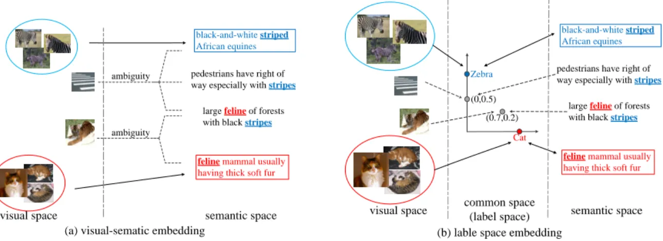
Fig. 1: The intuition of our method. “cat” and “zebra” are seen classes meanwhile “stride” and “tiger” are unseen classes. In the training phase, mappings denoted by the solid arrows are learned. In the testing phase, unseen images are projected by the leaerned mappings. (a) Learning visual-semantic embedding directly, correlations between prototypes may cause ambiguity. (b) Introducing the joint-label space makes prototypes more discriminative.
attributes into the same space (also called common space), a group of methods map both visual features and attributes into a common space, where low-rank condition can be added to restrict the common space [10] [11]. However, the optimal projection matrix may be not unique. For example, we denote matrix P as a linear embedding, which maps high dimensional vectors (i.e., denote to x1 and x2) from
the source space to the target space. Specifically, y1 = Px1
and y2 = Px2. And then, given arbitrary orthogonal matrix R, we have z1 = RPx1 and z2 = RPx2. It is easy to
be proved that the Euclidean distance or Cosine distance betweenz1andz2 are equal that ofy1andy2. In addition, to
preserve the structure of visual features in the common space, graph information, such as adjacent matrices, are generally considered [12] [13], which introduces large computational complexity. Besides, most existing methods directly connect features and attributes where the correlation among attributes in different classes can result in poor performance [14]. For example, if monkeys and bears are utilized as seen examples to train models, the property “brown” and “fur” are very relevant. As such, unseen animals having white fur such as “polar bears” may be considered completely different from seen classes. Consequently, reducing the correlation of classes can improve the discrimination of prototypes in the common space. Second, since the final classification is conducted in the semantic space in most methods, the gap between attributes and labels leads to significant performance degradation.
In this paper, we propose a novel ZSL framework by defin-ing a discriminative label space where the final classification is conducted. In this label space, labels of seen classes are fixed into one-hot vectors as references to decorrelate features and attributes. The labels of unseen classes are obtained by mapping class-level attributes into the label space. Since seen and unseen class labels are defined in different ways, they are more robust in the final classification. To train the embedding from visual space to common space, a linear projection matrix is learned to avoid over-fitting. To learn the embedding from semantic space to common space, the attribute and label of
the same seen class are required to reconstruct each other, because they hold equivalent class information. Since there is no additional constraint such as graph information, the computational complexity is very low in the training phase.
An illustration of our method is shown in Figure 1. Assume “cats” and “zebras” are two seen classes, while “tigers” and “street crossings” are unseen classes. If the visual-semantic embedding is learned directly, the correlations between the prototypes may lead ambiguity when classifying unseen im-ages. Differently, the prototypes of seen classes are firstly defined when the label space is used, and then unseen pro-totypes are learned by their relationship of corresponding seen prototypes, which can reduce the ambiguity caused by correlations. For example, both the image and texture de-scription of the class “street” crossing contain “stripes”; thus, both their projections in the label space refer to “zebras”. Similarly, “tigers” refer to both “cats” and “zebras” classes owing to their “feline” and “stripe” properties, respectively. More importantly, labels of seen classes are accurately defined as one-hot vectors; thus, seen and unseen classes in the label space are more discriminative in GZSL. We conduct experiments to compare the proposed method with state-of-the-art baselines under five benchmark datasets with the same features, splits and evaluation [15]. Results demonstrate the leading performance of our method in most cases, especially for the GZSL task.
Existing methods introducing class labels generally use them as indexes or regularization. For example, labels are regarded as indexes to the corresponding semantic attributes [16] [17]. Another way of using the labels is to utilize them in a regularization to learn parameters [18] [19]. Differently, class labels in this paper are directly regarded as variables, which are the targets of the projected visual features and semantic attributes. Thus, the influence of the class labels is much stronger than reference methods. A similar work is Indirect Attribute Prediction (IAP) [20] that establishes a probability model to predict attributes based on visual features, which generally requires a lower computational cost than the direct
attribute prediction [21]. However, labels of seen and unseen classes are defined in different spaces, which is not appropriate for the GZSL task. In [19], class labels are introduced to learn prototypes in the visual space. Labels are employed only as a constraint, and not as embeddings in this method, where the correlation between features and attributes still influences the learning of projections. In this paper, we define a complete label space, where both seen and unseen class centers are in the same space like traditional supervised classification. This paper makes three main contributions.
• Since a label space is employed to jointly connect the visual and the semantic space, the correlation in visual and semantic space is reduced in the label space, which results in performance improvement.
• In the testing phase, seen classes are also fixed to one-hot vectors, while unseen classes are computed by a learned model. Therefore, the label space where the final classification is conducted is robust.
• Detailed comparisons among different frameworks and mappings are discussed to show the advantages of intro-ducing and attributing the label space, especially for the GZSL task.
II. RELATEDWORKS
A. Embedding Learning
To train a model from seen classes that can be generalized to classify unseen classes, visual features, attributes and labels of seen classes are generally required. In the testing phase, test features should be classified into the correct classes identified by their attributes via the learned model. According to whether or not the label space is introduced as an intermediate space connecting the visual and semantic space, ZSL methods can be divided into Direct Visual-Semantic Embedding and Indirect Visual-Semantic Embedding frameworks.
Direct Visual-Semantic Embedding (DVSE): the DVSE
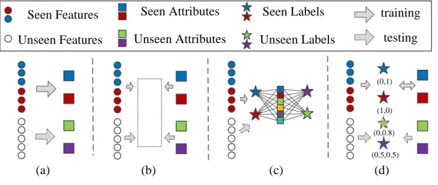
framework, containing most existing ZSL methods, directly estimates the conditional distribution or mapping between visual features and their corresponding attributes. There are three types of DVSE methods. The first category of methods train linear or nonlinear mappings, which transform features from the visual space into the semantic space [20] [22] [23] [24] [16] [25] [26]. Fig. 2(a) shows an illustration, where visual features and attributes of seen classes are collected to train mappings. In the testing phase, the similarity between images and prototypes of new classes in the semantic space is measured for classification. The second category of methods synthesize visual features with attributes [27] [28], which can reduce the hubness problem when the Nearest Neighbor (NN) search is used in the visual space for classification [29]. Alternatively, a supervised classifier can be trained with synthesized features instead of the NN search [30]. The pipeline of the second category is reverse is shown in Fig. 2(b). In the third category of methods, a common space is learned using features and attributes from seen classes [31] [32] [4] [33] [10], as shown in Fig. 2(c). To recognize images in unseen classes, both visual features and attributes are projected into the common space for NN search. The common space in Fig.
2(c) is represented by the dashed box, which indicates that the space is totally unknown and must be trained. Notice that, in Fig. 2(a), (b) and (c), class labels are only used to identify visual features and attributes in the same class (i.e., the same color), which are not regarded as variables.
Indirect Visual-Semantic Embedding (IVSE): In this
framework, labels of seen classes are used as intermediates to connect the visual and semantic space. The independence of labels in different classes can significantly reduce the correlation among dimensions in the semantic space, therefore, the mapping from images to classes is more discriminative. As illustrated in Fig. 2(d), IAP introduces the labels of seen classes as intermediate variables between features and attributes. When new attributes are obtained, the condition probabilities of attributes and labels in unseen classes are learned. The online incremental zero-shot learning method was proposed based on IAP [21], because it requires lower com-putational cost comparing to the Direct Attribute Prediction (DAP). Due to labels of seen and unseen classes are defined in two different spaces, IAP is not appropriate for the GZSL task.
In the proposed method, the label space is not only intro-duced to reconcile features and attributes, but also used for classification. As shown in Fig. 2(e), the label space contains priori seen labels and projected unseen labels. This is the main difference between IVSE and ALS. Specifically, labels of seen classes are fixed as one-hot vectors in the common space, and are represented by solid stars. Mappings are trained to project visual features and semantic attributes into their class labels. After training these mappings, attributes of test classes are mapped into the common space to act as labels for unseen classes, which are denoted by dashed stars.
Compared with the IAP method, there are three main differences. First of all, labels of seen and unseen classes are defined in the same space, so can be directly generalized to the GZSL task. Secondly, labels of seen classes are fixed as one-hot vectors, which are used to compose unseen labels. In this way, seen and unseen classes can be regarded as “pure substances” and “mixtures”, which is more discriminative in the GZSL task. Finally, labels and attributes are required to reconstruct each other in the training phase, which can reduce the domain shift problem between seen and unseen attributes.
B. Semantic Representation
There are mainly two ways to obtain the prototypes of classes in the semantic space for zero shot image classification. The first way is introducing labelled attributes, and each dimension of an attribute vector is a specific property. When these class-level attributes are regarded as class centers in the semantic space to classify images, it is similar to the multi-label classification task. In ZSL or GZSL task, it only required to label once for each class, then hundreds of unlabeled images can be classified into the new defined class. Even though, labeling attributes is more expensive than label single image in establish the dataset, therefore attributed-based ZSL is mainly used for small or medium datasets, such as Attribute Pascal and Yahoo (aPY) [34], Animals with Attributes (AWA) [15],
(a)
(b)
(c)
(d)
Seen Features
Seen Attributes
Unseen Features
Unseen Attributes
Seen Labels
Unseen Labels
training
testing
(0,1) (1,0) (0,0.8) (0.5,0.5)Fig. 2: Comparison of different ZSL frameworks. (a) Mapping visual features into the semantic space; (b) Mapping semantic attributes into the visual space (c) Common space embedding; (d) Indirect attribute prediction; (e) Attributing label space.
Caltech-UCSD-Birds (CUB) [35] and SUN attributes (SUN) [36].
Another way to obtain the semantic representation is us-ing vocab or sentence embeddus-ing extracted from the tex-ture description of classes. This way is more like to be a multimodality learning task [37], because measuring the similarity between visual and semantic spaces requires to align two modalities. Compared to labeling attributes, it requires little annotation information to extract semantic embeddings from pre-trained model using natural language processing techniques like BERT [8]. Therefore, it is mainly used for generate large-scale dataset for ZSL, like ImageNet [38]. However, two problems can influence the performance of the ZSL methods when sentence embeddings are used. Firstly, the texture description may be not strict or complete, which can introduce ambiguity. Secondly, there is the information loss of extracting features compared to directly label the attributes. Since the classification accuracy of ZSL is much less than that of supervised image recognition, existing methods including our work mainly focus on the attribute-based task, which is easier than using embeddings.
Early works for ZSL and GZSL do not have the same exper-imental setting thus the comparison results may be reasonable, therefore, authors in [15] propose a uniform setting and re-evaluate plenty of methods under their standard. In [15], class attributes in high dimensional vector are used as the semantic representations in aPY, AWA, CUB and SUN, meanwhile the sentence embeddings are regarded as the semantic represen-tations in ImageNet. To have a fair comparison with existing methods, we completely follow the experimental settings in [15], which are described in detail in the Section V.
III. APPROACH
In the zero-shot learning task, we aim to correctly recog-nize images in unseen classes according to their class-level attributes, where unseen classes are totally independent from the training phase.
Assume we have C seen classes to train the model. The training dataset Ds is defined by a series of triplets (xi
s,yis,ais) Ns
i=1 ∈ Xs×Ys×As, where Ns is the number
of training samples.Xs∈Rd×Ns denotes the set of images or
features.Ys∈ {0,1}C×Ns represents the one-hot class labels,
where one element of each column is 1, while the others are 0. As ∈ Rk×Ns contains training attributes. Note that
class-level attributes are used in this method, which means Ys and As are augmented from {0,1}C×C and Rk×C respectively,
by class labels. Moreover, in the training phase, the label (or common) space only contains C labels, which can be denoted asY∈ {0,1}C. Two models must be learned to map
features and attributes into the label space, respectively. In detail, f : xi
s → yis denotes the visual embedding, while
g : ai
s → yis is the semantic embedding. In the testing
phase, visual and semantic samples of unseen classes are given, i.e., (xi
u,aiu) Nu
i=1 ∈Xu×Au. Since labels of seen and
unseen classes are unified in the same space, the discrete space Y is extended to Y = RC, which is continuous and
has enough positions to represent the growing number of unseen classes in the common space. For classification, let
A= (a1, ...,aC,aC+1, ...,aC+U) denote class-level attributes inC seen andU unseen classes.
A. Attributing Label Space (ALS)
In this paper, we define the common space asRC, where
labels of seen classes are represented by one-hot vectors to reduce the correlation between semantic attributes. The loss function can be written as
min
P,Q f(Xs,Ys;P) +g(Ys,As;Q) + Ω(P,Q), (1) wherePandQare the parameters of the two mappings.Ω(.)
is the regularization. In Eq. (1), constraints can be introduced in regularization term to connect the two mappings.
Visual Embedding: In this paper, visual embedding aims
in the common space. A direct way of doing this is to train a classifier like SVM. For each feature, the score of the corresponding classifier is set to 1 while that of other classifiers is 0. However, for ZSL, using a classifier is not appropriate for visual embedding because it induces over-fitting. Specifically, typical classification methods can correctly map seen features to their labels. However, in the testing phase, unseen features are also mapped to those labels, which is meaningless for ZSL, because test features obviously do not belong to any known classes. In this method, our embedding only aims to map features in seen classes to the corresponding one-hot vectors, according to their class labels. Therefore we simply letf be a linear projection, where labels of unseen classes are represented as linear combinations of one-hot vectors, instead of a one-hot vector itself.
Semantic Embedding: Generally, semantic embedding is
used to adjust the relative positions of prototypes, which should be the centers of projected features. In this method, because the correlation among dimensions of semantic space tend to mislead the visual embedding learning, we regard the semantic embedding as a decorrelation process. In other words, attributes in different classes should be more indepen-dent in the common space. To this end, we directly map an attribute to the corresponding one-hot vector in the label space. Besides, since there is a one-to-one correspondence between an attribute and its class label, we assume that if a semantic attribute is mapped to a label, then it can also be reconstructed from the label by inverse operation.
From the above discussion, the objective function of the proposed method can be defined as
min P,Q||PXs−Ys|| 2 F +||Ys−QTAs||2F+α||P|| 2 F +β||Q|| 2 F, s.t. As=QYs, (2) whereP∈RC×d andQ∈
Rk×Cdenote the linear visual
em-bedding and visual emem-bedding, respectively. Here, we simply use the L2 norm as the regularization of two projections. In the training phase,PandQcan be optimized individually. Let the gradient of P for Eq. (2) equal zero, the closed form of visual embedding is
P=YsXTs(XsXTs +αI)
−1. (3)
For semantic embeddingQ, we relax the constraint and the objective function related to Qcan be rewritten as
min Q ||As−QYs|| 2 F+λ||Ys−QTAs||2F+β||Q|| 2 F, (4)
whereλis a weighting coefficient that balances the importance of the first and second terms. The derivation of Eq. (4) is
λAsATsQ+Q(YsYTs +βIC×C) = (1 +λ)AsYTs. (5)
Eq. (5) is the Sylvester Equation [39], which has the closed form solution
vec[Q] =[IC⊗(λAsATs) + (YsYTs +βIC×C)⊗Ik]−1
vec[(1 +λ)AsYTs],
(6)
wherevec[Q] is the vectorization operation for matrix Q, ⊗
denotes the Kronecker product and Ik stands for the k×k
identity matrix.
Since the main computational cost comes from solving the Sylvester Equation, the proposed method has similar computational complexity as SAE [40], which can be trained very quickly.
B. Classification
In the training phase, the common space Y contains C one-hot vectors. When unseen classes are observed in the testing phase, their attributes are projected into the common space as labels of unseen classes. Moreover, for real-world recognition tasks, the number of new classes is unknown, and even rises over time. To solve this problem, the common space is extended as Y = RC, where infinite prototypes can be
defined in the continuous space. In ZSL, givenU attributes of unseen classes aj (j ∈ C+ 1, ...C+U), their labels in the common space are represented as
ljz=QTaj, j =C+ 1, ..., C+U. (7) In our method, the classification is based on NN search in the common space, c(xiu) =argmin j d(Px i u,l j z), j∈C+ 1, ..., C+U, (8) where c(xi
u) is the class identity of unseen sample xiu, and
d(a,b)denotes the distance between vectora andb.
In the testing phase of GZSL, labels of unseen classes are similar to those for ZSL. Different from existing methods, labels of seen classes are denoted as the one-hot vectors. In this way, labels of GZSL are defined as
ljg=
yj, j = 1, ..., C
QTaj, j =C+ 1, ..., C+U, (9)
whereyj denotes the label of thej-th seen class. The
classi-fication of GZSL is also based on the NN search, c(xiu) =argmin j d(Px i u,l j g), j ∈1, ..., C+U. (10)
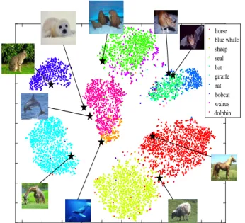
As labels of seen classes are exact one-hot vectors in Eq. (9), the label space is more accurate for representing both seen and unseen classes. This is the main reason why ALS makes significant improvement in GZSL. In addition, for human beings, a general way to define objects in new classes is to combine properties of known classes [20]. For example, “motor homes” contain a similar shape and function as both “motor” and “house”. In other words, meanings are given to labels of unseen classes in the original label space. In this way, the model recognizes new classes as analogy of seen classes, which is more natural. Example from the dataset Animals with Attributes (AWA) [15] are shown in Figure 3. In detail, six classes are selected as seen classes that vary in shape, size, life habit, etc. Thus, each class is assumed to be orthogonal to the others. The t-SNE result [41] of visual features projected in the label space is shown, where labels of six seen classes are fixed to one-hot vectors, which further make up labels of three unseen classes. Specifically, the unseen object “giraffe”
antelope killer whale gorilla rabbit otter cow giraffe rat dolphin
Fig. 3: Relationship between six seen and three unseen classes illustrated by t-SNE. Projected features of seen classes in the common space are represented by “+”, while the corresponding images are in solid boxes. Features in unseen classes are denoted by “.”, while images are in dashed boxes. Arrows denote axes in the common space
can be regarded as the linear combination of “antelope” and “cow”, because the shape of giraffes is similar to antelopes, while both giraffes and cows have spots. Similarly, “rat” is correlated to both “rabbit” and “otter”. In contrast, a “dolphin” is more similar to a “killer whale” than any other seen classes so its label is only near to that of the killer whale. Besides, all unseen labels are far from the “gorilla” since they have few common attributes. This result verifies our assumption about the relationship between prototypes of seen and unseen classes. In Figure. 4, t-SNE projections in the common space of all 10 unseen classes are shown. In most cases, features and attributes in same classes are projected into the same regions. This demonstrates that the label space can efficiently reconcile visual and semantic spaces.
IV. MODELANALYSIS
After establishing the ZSL model, we further analyze dif-ferent frameworks of learning embeddings for ZSL, where the direction of inference is discussed in detail. As we mainly focus on discussing of the framework rather than specific approaches in this section, linear projections are used for fair comparison. All comparisons that verify our conclusions in this section are shown in Section V.
A. Comparison of Different Frameworks
In this paper, different frameworks are discussed and com-pared. Methods that directly learn mappings between the visual and semantic spaces belong to the DVSE framework, where class labels are not introduced. Differently, methods in IVSE use the labels of seen classes as variables, but the final classification is not conducted in the label space. In contrast, the compatibility function of the proposed ALS is directly
horse blue whale sheep seal bat giraffe rat bobcat walrus dolphin
Fig. 4: The t-SNE projection of visual features projected in the label space. Visual points are denoted by “.” and semantic prototypes are represented by stars.
defined in the label space, where both seen and unseen classes are unified.
In the DVSE framework, “visual projection” is the direct method, where the training phase can be defined as
min P ||PXs−As|| 2 F +α||P|| 2 F. (11)
In the following discussion, Eq. (11) is denoted as “X→A”, where features are projected into the semantic space for NN search. A main disadvantage is that visual projection tends to cause the hubness problem [27], where most projected features share the same prototype as their nearest neighbor. According to [42], the reverse process of visual projection can reduce the hubness problem, i.e.,
min P ||Xs−PAs|| 2 F +α||P|| 2 F, (12)
which is represented as “X←A”. As attributes are projected into the visual space, this is also called “visual synthesis” [30], where visual features of unseen classes can be synthesized by their attributes from projection P. However, because the distribution of visual features in seen and unseen classes are generally different, unidirectional projections in Eqs. (11) and (12) induce the domain shift problem [43]. To solve this problem, the “mutual reconstruction” is defined as
min P ||Xs−PAs|| 2 F +α||P TX s−As||2F, (13)
where visual features and semantic attributes are required to reconstruct each other with the same parameters P. In [40], a projection trained by Eq. (13) is proved to be efficient to reduce the domain shift problem. In addition, the final classification can be conducted in either the semantic or visual space, where the corresponding compatibility function is defined as d(PTxiu,aj) or d(xiu,Paj). For convenience of
ˆ
A andXˆ mean the classification is implemented in semantic and visual space respectively.
In our experiments, the classification accuracies of these four strategies are compared. We find that, X← A is much better than X → A, while, X ↔ Aˆ and Xˆ ↔ A are better than X→ Aand X←A, respectively. According to related experiments in Section 4.3, two conclusions are verified. First, when mutual reconstruction is introduced, the classification accuracy is generally increased because the domain shift problem is reduced. Second, the hubness problem can be reduced when classification is conducted in the visual space.
When the label space is introduced as an intermediate space, Eq. (11-13) can be respectively modified as
min P,Q ||PXs−Ys|| 2 F+α||P||2F+||QYs−As||2F+β||Q||2F, (14) min P,Q ||Xs−PYs|| 2 F+α||P|| 2 F+||Ys−QAs||2F+β||Q|| 2 F, (15) min P,Q||Xs−PYs|| 2 F+α||P T Xs−Ys||2F +||As−QYs||2F+β||Q T As−Ys||2F. (16)
In Eq. (14), features are projected into the semantic space via mappings P and Q, denoted by “X → Y → A”. In the testing phase, the compatibility function isd(QPxiu,aj), which
is defined in the semantic space. After training via Eq. (15), NN search is implemented in the visual space where attributes are mapped, and this process is denoted by “X← Y←A”. Similar to Eq. (13), there are three classification methods when
PandQare trained via Eq. (16). Specifically, “X↔Y↔Aˆ” and “Xˆ ↔Y↔A” denote that the classification is conducted in the semantic and attribute space, respectively. As such, prototypes cannot be fixed to one-hot labels, so attributes or synthesized features are used as prototypes. In detail, compat-ibility functions are respectively defined asd(QPTxi
u,aj)and
d(xi u,PQ
T
aj). Both these strategies belong to IVSE according
to our definition. Differently, when the label space is directly used for NN search via Eqs. (8) and (10), “X↔Yˆ ↔A” is a typical model in ALS.
Based on comparisons in our experiments, two conclusions can be drawn. Primarily, introducing the label space can decrease the correlation among properties (dimensions) in the semantic space. Therefore, two projectionsPandQare more discriminative, and projected features from different classes can be divided easily. This is demonstrated by the fact that IVSE is better than DVSE in the same cases. Besides, ALS defines a robust common space where seen prototypes are one-hot vectors and unseen prototypes are infered by semantic embedding. In this way, priori knowledge of seen class labels is used to accurately define the label space, making prototypes in the common space more discriminative. This is the main reason that the ALS framework performs much better than IVSE for the GZSL task. This is verified by the fact that
X ↔ Yˆ ↔ A is much better than X ↔ Y ↔ Aˆ and
ˆ
X ↔ Y ↔ A for the GZSL task. Relevant comparisons are shown in Section V.
B. Comparison of Mappings
After showing the improvements of ALS, the influence of different projection directions in the ALS framework is also considered. In this Section, the final classification is conducted in the label space in all cases.
Our main model is defined as (2), which can be denoted as “X → Y ↔ A”. As we first discuss the different way of semantic embeddings, the visual embedding is fixed as “X → Y”. As attributes of unseen classes are projected into the label space, there are two different directions, label synthesis “Y ← A” and mutual reconstruction “Y ↔ A”. For a given class, the label and class-level attributes hold the same information when they are used as class centers. In addition, in the proposed method, semantic meanings are given to labels. Consequently, it is more reasonable that labels and attributes in the same class are required to reconstruct each other. Moreover, because the number of training classes is generally small, and the distributions between attributes in seen and unseen classes are very different, the domain shift problem causes degradation if a mapping from attributes to labels is trained directly. The mutual reconstruction loss can prevent the over-fitting in the training phase in this way.
Similarly, the semantic embedding is fixed as “Y↔A” and different methods of visual embedding are compared: “X → Y” and “X ↔ Y”. Notice that X ↔ Y requires labels to reconstruct visual features, and contains the term
γ||Xs−PYs||2F =γ C X c=1 X xi s∈Xcs ||xi s−Py c s|| 2 F, (17) where Xs = S C c=1X c
s denotes the partition of features in C
classes. Asycsis the one-hot vector indicating thec-th column
Pc, the optimal ofPc is the mean of features in thec-th class
Pc= ¯xc= 1 nc X xi s∈Xcs xis, (18)
where nc is the number of features in the c-th class. This
means that the label tends to be projected into the center of features in the visual space, because visual features in one class are much more diverse than their class labels. According to Eqs. (17) and (18), the reconstruction loss has a lower bound
γ C X c=1 X xi s∈Xcs ||xi s−¯x c||2 F. (19)
When optimizingP, the lower bound can influence the optimal solution according to the hyper-parameter γ. In experiments, we find thatγhas a negative correlation with the classification accuracy. Therefore, it may not appropriate to reconstruct features from a single one-hot label vector. Detailed results are shown in the next Section, which demonstrate the above discussions of mapping selection.
C. Analysis of Hubness
Authors in [42] give the theoretical analysis why visual synthesis is better than visual projection. Specifically, if a linear embedding is learned via Eq. (11), it can be proved that
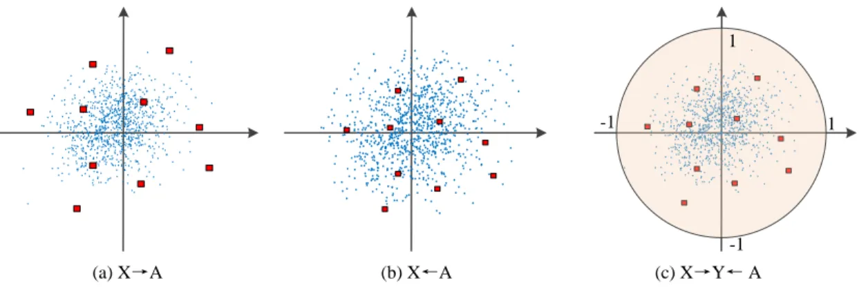
(a) X→A (b) X←A (c) X→Y← A
1 -1
-1 1
Fig. 5: Illustration of shrinkage. (a) Visual projection; (b) Visual synthesis; (c) Attributing label space.
||PXs||2F ≤ ||As||2F. This means that the projected pointsPXs
will be shrunk towards the targets As. Based on this proof,
the authors draw a conclusion that the influence of shrinkage will be reduced if the prototypes are in the visual space [42]. In our framework, both the visual features and semantic attributes are projected into the label space. When the model is trained via following function,
min P,Q ||PXs−Ys|| 2 F+α||P|| 2 F+||Ys−QAs||2F+β||Q|| 2 F, (20)
it can be easily proved that||PXs||2F ≤ ||Y|| 2
F and||QAs||2F ≤ ||Y||2
F. Therefore, there is no direct relationship of value
between||PXs||2F and||QAs||2F. It may be also a way to avoid
the influence of shrinkage, which is shown in Fig. 5. However, we find it is hard to have a theoretically proof of the relation-ship in norm in the Eq. (2). Thus, we compute ||QtA
s||2F for
all datasets and empirically find that ||QtAs||2F ≤ ||Y||2F is
also satisfied.
To further verify the ability of ALS to avoid the hubness problem, we introduce the “skewness” that measures the degree of hubness in a nearest neighbor search problem [29] [27], which is defined as skewness= PC c=1(Nk(c)−E[Nk]) 3/C V ar[Nk]3/2 , (21)
where theNk is the discrete distribution of the numberNk(c)
of the times each prototypecfound in the topkof the ranking for test samples. Notice that when k= 1,Nk represents the
distribution of the (predicted) labels of the test set. V ar[Nk]
is the variance of Nk. In experiments, the comparison of
skewness value in different frameworks are shown to verify the ability of our method to avoid hubness problem in the ZSL task.
V. EXPERIMENTS
In our experiments, our method is compared with state-of-the-art baselines on five benchmark datasets, including four medium-scale datasets and one very large-scale dataset under the same settings. To begin with, datasets, splits and other settings are introduced. Then the proposed method is evaluated
on the medium-scale datasets in detail, including a comparison of main accuracy with other baselines, discussion on different frameworks, the computational cost, and the influences on hyper-parameters. At last, our method is generalized to the large-scale dataset, which is very challenging for the GZSL task.
A. Datasets, Evaluations and Baselines
The medium benchmark datasets include Attribute Pascal and Yahoo (aPY) [34], Animals with Attributes (AWA) [15], Caltech-UCSD-Birds (CUB) [35] and SUN attributes (SUN) [36]. The very large-scale dataset is ImageNet 21K. aPY contains 15,339 images in 32 classes, with 20 seen and 12 unseen classes. Each class corresponds to a 64-dim attribute. For AWA, the original dataset [20] is not publicly available. Therefore, images in same classes are re-collected for training and testing [15]. AWA has a total of 37,322 images and 85-dim class-level attributes, in which 40 classes are used for training and 10 for testing. CUB contains 11788 images from 150/50 seen/unseen types of birds, where each type is described by a 312-dim attribute. SUN contains 14,340 images and 102-dim attributes, where 645 out of 717 classes are used in the training phase. To split the dataset for training and testing, we follow the settings in [15], where unseen classes are not included in the deep neural network training. Therefore, unseen classes are really “unknown” for the trained model. The 2048-dim feature of each image is extracted from the 101-layered ResNet [44]. Detailed splits of these datasets are shown in Table I.
The method is also tested on the large-scale dataset Im-ageNet, which contains 21,841 classes with more than 10 millions images collected from the real-world. In the training phase, 1K seen classes containing 1.2 million images are used to learn mappings, where the original ResNet-101 pre-trained on ImageNet is used to extract the 1024-dim visual features. In the testing phase, different splits are used as unseen classes. Particularly, 2-hop/3-hop contains 1,509/7,678 unseen classes that are within two/three tree hops of 1K seen classes according to the ImageNet label hierarchy [31]. Classes that contain the top 500/1K/5K maximum images as well as the top 500/1K/5K minimum images are also used for
TABLE I: Details of five datasets Dataset Dim. of at-tributes No. of seen classes No. of seen images No. of unseen classes No. of unseen images SUN 102 645 10320 72 1440 CUB 312 150 7057 50 2967 AWA 85 40 23527 10 7913 aPY 64 20 5932 12 7924 ImageNet 500 1K 1.2M 20K 10M
TABLE II: Comparisons of Zero-Shot Learning (ZSL) on SUN, CUB, AWA and aPY. We measure the AP of Top-1 accuracy in %.
method SUN CUB AWA aPY
DAP [20] 39.9 40.0 46.1 33.8 IAP [20] 19.4 24.0 35.9 36.6 CONSE [46] 38.8 34.3 44.5 26.9 CMT [24] 39.9 34.6 37.9 28.0 SSE [32] 51.5 43.9 61.0 34.0 LATEM [23] 55.3 49.3 55.8 35.2 ALE [4] 58.1 54.9 62.5 39.7 DEVISE [16] 56.5 52.0 59.7 39.8 SJE [22] 53.7 53.9 61.9 32.9 ESZSL [47] 54.5 53.9 58.6 38.3 SYNC [31] 56.3 55.6 46.6 23.9 SAE [40] 59.7 50.9 66.0 35.1 LESAE [11] 60.0 53.9 68.4 40.8 PSR [48] 61.4 56.0 63.8 38.4 SP-ANE [49] 59.2 55.4 58.5 24.1 ZSKL [50] 60.4 49.3 69.9 41.9 CDL [19] 63.6 54.5 69.9 43.0 MIVSE [17] 43.5 35.7 46.1 32.8 GCN [18] 48.8 48.9 54.6 40.38 ALS 62.0 57.5 66.2 44.5
testing respectively, which are represented as the 500/1K/5K most/least populated classes in experiments. Finally, all 20K classes are tested, which is very challenging. For each class, a 500-dimensional attribute is extracted using the “word-to-vector” method [45], since ImageNet does not contain attribute annotations for all classes. Details are shown in [31] and [15]. To evaluate the performance of the methods, the average of per-class precision (AP) is measured. Specifically, “zsl” denotes the AP of features classified into unseen classes. In the GZSL task, test features of unseen classes are classified into all classes, which is denoted as “ts”. In [15], a subset of features from seen classes are used for validation, which are also classified into both seen and unseen classes. The AP of these features is represented as “tr”. Finally, “H” is the harmonic mean of ts andtr, which is also introduced to evaluate the GZSL [15].
For comparison, a number of baselines in the (generalized) zero-shot learning task are introduced following [15], which include DAP [20], IAP [20], CONSE [46], CMT [24], SSE [32], LATEM [23], ALE [4], DEVISE [16], SJE [22], ESZSL [47], SYNC [31] and SAE [40]. Moreover, recent works such as LESAE [11], PSR [48], SP-ANE [49], ZSKL [50] and CDL [19] are also compared. Since recent works are seldom eval-uated in large-scale dataset ImageNet with standard settings, we only select the same methods as [15] to be baselines.
B. Main Results
We compare our approach with state-of-the-art baselines on five medium-scale datasets. In Table II, ZSL classification
-0.1 0 0.1 0.2 0.3 0.4 0.5 lion foxzebr a gian t pa nda elep hant gori lla hum pbac k w halecoli e cow buff alodeer rhin ocer os wol f ante lope siam ese cat wea selpig pers ian cat racc oon chih uahu a griz zly bear chim panz ee squi rrel germ an s heph erd pola r be ar otte r dalm atia n leop ard rabb it hipp opot am us ham ster ox skun k tige r kill er w hale spid er m onke y moo se mou se beav er mol e P ro je c te d a tt ri b u te o f d o lp h in -0.1 0 0.1 0.2 0.3 0.4 0.5 lion foxzebra gian t pa nda elep hant gori lla hum pbac k w halecoli e cow buff alo deer rhin ocer os wol f ante lope siam ese cat wea selpig pers ian cat racc oon chih uahu a griz zly bear chim panz ee squi rrel germ an s heph erd pola r be ar otte r dalm atia n leop ard rabb it hipp opot am us ham ster ox skun k tige r kill er w hale spid er m onke y moo se mou se beav er mol e M e a n o f p ro je c te d v is u a l fe a tu re s o f d o lp h in
Fig. 6: Correlations between unseen class “dolphin” and seen classes in the common label space.
-150 -100 -50 0 50 100 150 -150 -100 -50 0 50 100 150
Fig. 7: t-SNE visualization of projections in 50 in CUB dataset.
results are shown, where ‘ALS’ represents the result of our method. The accuracies of most baselines are tested in same settings as [15] for fair comparison. The proposed method achieves state-of-the-art performance on all four datasets, especially in terms of aPY. In CDL, the class labels are also introduced to learn a representation of visual features. And then the representations and semantic attributes are mapped into a common space. In fact, the pipeline of CDL in the
reason why these two methods achieve comparable accuracies. However, since we compute the similarity in the label space, the seen and unseen prototypes can be defined differently like Eq. (9). On contract, prototypes in seen and unseen classes in common space are computed in the same way in CDL. This is the mean reason that our method is better in the GZSL task. In summary, the model trained using seen data can be well generalized to unseen classes. An example from the AWA dataset can be found in Fig. 6, which shows the correlation between the unseen “dolphin” and forty seen bases in the label space. Since there are multiple images of dolphins, we compute the mean of features projected in the label space. Results show that dolphin has strong correlations with aquatic animals. More importantly, the projected feature center is similar to the projected attribute, which demonstrates that the proposed model can associate the visual and semantic space in the latent space. To further verify this conclusion, the t-SNE result of projections in 50 unseen classes in CUB is shown in Fig. 7, where the colored circles with black border denote the projected attributes in different classes, and the dots in different colors denote the projected visual features. Results show that most of the projected visual features and attributes are close in the common space.
For the GZSL task, the proposed method significantly im-proves thetsandH. The average increment oftsvalue is 11.2. TheHvalue jointly considers the classification performance of seen and unseen classes, which can be used as the evaluation for annotating new objects. Compared with state-of-the-art methods, the H value is increased by 4.7, 0.5, 8.3 and 11.9 on SUN, CUB, AWA and aPY, respectively. tr reflects the over-fitting training for seen classes. In Table III, the baselines with the highest tr generally refer to very low ts and H
values. This means the trained model in these methods cannot be generalized to new classes. Compared with baselines, the proposed method achieves leading performance considering in recognizing both seen and unseen classes.
C. Detailed Evaluation
In this section, detailed results for the model analysis are shown, where zsl and H represent the performance for the ZSL and GZSL tasks, respectively. A comparison of Eqs. (11-13) is shown in the first row of Table IV. Mappings of both
X↔Aˆ andXˆ ↔Aare trained via Eq. (13). They implement classification in the semantic space Aˆ and visual space Xˆ
respectively. Results demonstrate that X←A is much better than X→A, which verifies that visual synthesis can reduce the hubness problem. In addition, the mutual reconstruction can reduce the domain shift problem, suggested by the fact that results of X ↔ Aˆ andXˆ ↔ A are better than those of
X→Aand X←Arespectively. More importantly, compar-isons between DVSE and IVSE demonstrate an improvement when label space is introduced, where zsl andH values rise in most cases. Last but not least, although trained via Eq. (16), accuracies are different when the final classification is conducted in each of the three different spaces. ALS, where the compatibility function is defined in the label spaceYˆ, achieves
ˆ
X↔Y ↔Aand X↔Yˆ ↔ Aˆ. This verifies the advantage
of priori seen labels in generalized zero-shot classification. The accuracy of different mapping directions are also shown. The results shown in the first row of Table V verify that mutual reconstruction between labels and attributes can reduce the domain shift problem, since the results ofX→Y↔Aare better than that of X→Y←A. In the second row of Table V, the two visual embedding methods achieve comparable accuracy, while the visual projection X → Y obtains the leading performance in most cases. For X ↔ Y ↔ A, the hyper-parameter γ in Eq. (17) is set to a very small value, i.e, from 0.001 to 0.1, according to different datasets. In fact, γ has a negative correlation with accuracy, which means the reconstruction of visual features can degrade in performance as γrises. SinceX→Y↔Aachieves the leading performance, its accuracy is recorded as our main result in comparison in Table III.
Moreover, the comparison between the non-linear embed-ding and the linear embedembed-ding under our ALS framework is presented in Table VI, where the GZSL accuracies are eval-uated. Specifically, for visual embedding, we use three Fully Connected layers which are followed with Batch Normaliza-tion (BN) [51] and ReLU [52] layers. For semantic embedding, the Auto-Enocoder structure is introduced, where the codes of class-level attributes are required to be near to corresponding class labels as much as possible. The experimental results show that non-linear embedding achieves higher accuracies intr. It is because that the non-linear embedding tends to let unseen images directly equal to the defined one-hot labels, which causes overlap between seen and unseen projections in the common space. In fact, unseen features are mapped among the one-hot labels (as their linear combinations), not directly equal to one-hot labels. The results also verify our analysis in Section III-A.
Finally, to verify the ability of avoiding hubness problem of different frameworks, we compute the skewness value, where the distribution ofN1 is used. Since the number of samples in
each class in SUN dataset exactly equals to 20, the skewness value computed via the definition is not a number, because both the numerator and denominator are 0. Therefore, we use the variance of the distribution of predicted labels to instead skewness value in SUN dataset. The results show that the skewness value of the proposed method is closer to that of the ground truth in most cases. Notice that the number of images in each class is not balanced in APY, therefore, the skewness value of ground truth is the biggest.
D. Influence of Hyper-parameters
In our method, there are three hyper-parameters α, β and λ, which balance the influence of the regularization terms in the objective functions. In this section, the influence of the hyper-parameters is discussed to demonstrate the robustness of proposed method. We vary one hyper-parameter at a time, while fixing the others. The influences ofα,β andλ, for the four medium-scale datasets are shown in Figure 8. As can be seen, none of the parameters have a significant influence for
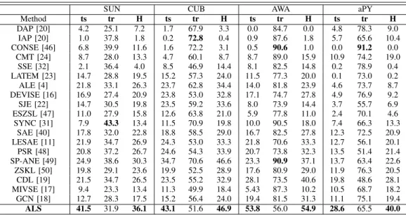
TABLE III: Generalized Zero-Shot Learning (GZSL) results on SUN, CUB, AWA and aPY. (CMT*: CMT with novelty detection). We measure the AP of Top-1 accuracy in %.
SUN CUB AWA aPY
Method ts tr H ts tr H ts tr H ts tr H DAP [20] 4.2 25.1 7.2 1.7 67.9 3.3 0.0 84.7 0.0 4.8 78.3 9.0 IAP [20] 1.0 37.8 1.8 0.2 72.8 0.4 0.9 87.6 1.8 5.7 65.6 10.4 CONSE [46] 6.8 39.9 11.6 1.6 72.2 3.1 0.5 90.6 1.0 0.0 91.2 0.0 CMT [24] 8.7 28.0 13.3 4.7 60.1 8.7 8.7 89.0 15.9 10.9 74.2 19.0 SSE [32] 2.1 36.4 4.0 8.5 46.9 14.4 8.1 82.5 14.8 0.2 78.9 0.4 LATEM [23] 14.7 28.8 19.5 15.2 57.3 24.0 11.5 77.3 20.0 0.1 73.0 0.2 ALE [4] 21.8 33.1 26.3 23.7 62.8 34.4 14.0 81.8 23.9 4.6 73.7 8.7 DEVISE [16] 16.9 27.4 20.9 23.8 53.0 32.8 17.1 74.7 27.8 4.9 76.9 9.2 SJE [22] 14.7 30.5 19.8 23.5 59.2 33.6 8.0 73.9 14.4 3.7 55.7 6.9 ESZSL [47] 11.0 27.9 15.8 12.6 63.8 21.0 5.9 77.8 11.0 2.4 70.1 4.6 SYNC [31] 7.9 43.3 13.4 11.5 70.9 19.8 10.0 90.5 18.0 7.4 66.3 13.3 SAE [40] 17.8 32.0 22.8 18.8 58.5 29.0 16.7 82.5 27.8 12.3 72.5 20.9 LESAE [11] 21.9 34.7 26.9 24.3 53.0 33.3 21.8 70.6 33.3 12.7 56.1 20.1 PSR [48] 20.8 37.2 26.7 24.6 54.3 33.9 20.7 73.8 32.3 13.5 51.4 21.4 SP-ANE [49] 24.9 38.6 30.3 34.7 70.6 46.6 23.3 90.9 37.1 13.7 63.4 22.6 ZSKL [50] 19.8 29.1 23.6 19.9 52.5 28.9 17.6 80.9 29.0 11.9 76.3 20.5 CDL [19] 21.5 34.7 26.5 23.5 55.2 32.9 28.1 73.5 40.6 19.8 48.6 28.1 MIVSE [17] 9.4 23.3 13.4 11.3 49.9 18.4 5.43 87.3 10.2 10.5 68.7 18.2 GCN [18] 12.7 28.3 17.5 15.2 56.4 24.0 19.4 81.5 31.3 11.1 75.1 19.4 ALS 41.5 31.9 36.1 43.1 51.6 46.9 53.8 56.0 54.9 28.6 65.5 40.0
TABLE IV: Comparison between DVSE and IVSE frameworks on SUN, CUB, AWA and aPY. We measure the AP of Top-1 accuracy in %.
SUN CUB AWA aPY
Framework Projections zsl H zsl H zsl H zsl H DVSE X→A 44.8 16.2 35.7 21.4 51.8 22.4 29.6 20.3 X←A 60.8 24.2 51.9 30.0 65.5 37.7 41.7 21.0 X↔Aˆ 53.5 17.9 36.4 23.3 57.1 23.1 29.0 9.3 ˆ X↔A 61.0 25.0 51.9 29.0 66.0 29.4 35.1 21.9 IVSE X→Y→A 44.8 16.4 36.2 21.6 54.8 24.4 29.7 22.3 X←Y←A 61.2 24.2 52.4 30.2 65.9 40.1 42.9 22.4 X↔Y↔Aˆ 56.3 17.6 46.7 23.8 58.9 36.8 33.7 13.3 ˆ X↔Y↔A 60.1 24.8 53.7 33.1 65.4 36.9 38.6 25.9 ALS X↔Yˆ↔A 61.5 36.1 54.9 40.4 64.6 53.9 42.3 38.8
TABLE V: Comparison of projection selections on SUN, CUB, AWA and aPY. We measure the AP of Top-1 accuracy in %.
SUN CUB AWA aPY
Projections zsl H zsl H zsl H zsl H
X→Y←A 61.7 35.6 55.9 46.1 59.3 21.1 41.2 22.0
X→Y↔A 62.0 36.1 57.5 46.9 66.2 54.9 44.5 40.0
X↔Y↔A 61.5 35.1 54.9 40.4 64.6 53.9 42.3 38.8
X→Y↔A 62.0 36.1 57.5 46.9 66.2 54.9 44.5 40.0
SUN and aPY. However, the accuracy on CUB decreases asα rises, while performances on AWA and CUB have a negative correlation withλ.
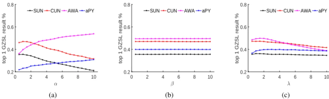
For the GZSL task, the H value is shown in Fig. (9). β is very robust for all datasets. Moreover, when λ is in the range [1.0 2.0], the best performance is obtained for all four datasets. In contrast, accuracies are very different as α changes. Specifically, the H value of AWA and aPY has a positive correlation with α, while that of SUN and CUB is negative. Considering the trade-off in both the ZSL and GZSL tasks, λ can be empirically set in the range of [2.0, 4.0], while β is fixed to 1.0. α varies from 1 to 100, according to different datasets. In Eq (2), the error of||Px–y||2
F will get
larger as α rises in α||P||2
F, which means the projection of
seen classes will leave far away from one-hot labels. In our ALS framework, the prototypes in seen and unseen classes are
defined in different ways that is show in Eq. (9). In this way, the improvement ofαmay increasetsand decreasetr, which will further cause salient change of the Hvalue. Differently, semantic embedding Q is constrained by the reconstruction error, therefore the hyper-parameterβ or γdo not cause such large variety. Moreover, the harmonic meanHvalue is a trade-off between ts and tr, where a maximum is existed in each dataset. In SUN and CUB, the maximum ofHvalue appears when αis near to 1. In AWA and APY, the maximum of H
value appears when αis larger than 10.
E. Computational Cost
It is very efficient to train projections in SAE [40], where the main cost comes from solving the Sylvester Equation. Specifically, the computational complexity isO(d3k3), where dandkare the dimensions of the visual and semantic spaces,
in %.
SUN CUB AWA aPY
Method ts tr H ts tr H ts tr H ts tr H Non-linear ALS 2.1 32.7 0.04 3.1 56.3 0.04 3.1 83.4 0.06 5.3 81.6 0.1 Linear ALS 41.5 31.9 36.1 43.1 51.6 46.9 53.8 56.0 54.9 28.6 65.5 40.0 0 2 4 6 8 10 0.4 0.6 0.8 top 1 ZSL result %
SUN CUN AWA aPY
(a) 0 2 4 6 8 10 0.4 0.6 0.8 top 1 ZSL result %
SUN CUN AWA aPY
(b) 0 2 4 6 8 10 0.4 0.6 0.8 top 1 ZSL result %
SUN CUN AWA aPY
(c)
Fig. 8: ZSL accuracy of the proposed method, influenced by hyper-parametersα, βandλ.
0 2 4 6 8 10 0.2 0.4 0.6 0.8 top 1 GZSL result %
SUN CUN AWA aPY
(a) 0 2 4 6 8 10 0.2 0.4 0.6 0.8 top 1 GZSL result %
SUN CUN AWA aPY
(b) 0 2 4 6 8 10 0.2 0.4 0.6 0.8 top 1 GZSL result %
SUN CUN AWA aPY
(c)
Fig. 9: GZSL accuracy of the proposed method, influenced by hyper-parametersα,βandλ
TABLE VII: Comparison of skewness value of different frameworks.
Framework SUN* CUB AWA aPY
X→A 264.7 1.26 1.99 0.46
X←A 42.3 0.68 1.17 1.45
X→Y↔A 39.0 0.71 0.62 1.79
ground truth 0 -3.82 0.23 2.62
TABLE VIII: Comparison of computational cost between the pro-posed method and SAE. We measure time consumption in seconds.
method SUN CUB AWA aPY
SAE 1.97 2.72 2.44 1.64
ALS 1.66 1.07 3.12 1.57
respectively. In the proposed method, the computational com-plexity for solving Eq. (6) is O(C3k3), where C is the
number of seen classes. In real applications, visual features are extracted from deep networks, and d is generally bigger thanC. Therefore, the proposed model is comparable and even faster than SAE for projection training. The costs for each dataset are listed in Table VIII. Results show that our method has similar time consumption with SAE to learn projection matrices.
F. Large-scale Dataset
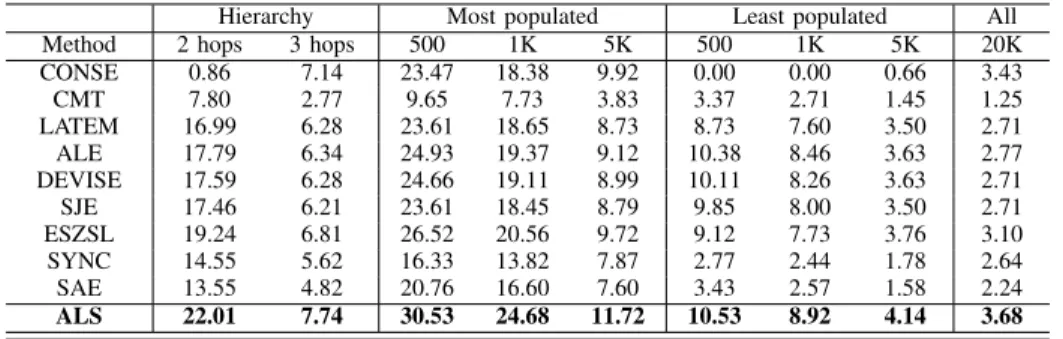
Finally, our method is evaluated on the ImageNet 21K dataset, where the top-10 accuracy is computed. Comparisons for the ZSL task are shown in Table IX, where we choose the same baselines as [15]. Our method is better than most baselines and is comparable to the current state-of-the-art performance. More importantly, the proposed method achieves the leading performance in least populated 500/1K/5K classes. This means that our method is advantageous for annotating images of objects that are rare in nature, which is the original intention of ZSL. For the GZSL task, the evaluation of “ts” is presented in Table X. Results show that the proposed method achieves state-of-the-art performance in all cases, especially for 2 hops and most 500/1K unseen classes, where about 3-4 increments are achieved. All results demonstrate the advantage of our method for GZSL. Since the sentence embedding of texture description of classes are used, it is different from the attribute-based ZSL as we mentioned in the Section I and Section II. This is the reason that the accuracy of our method is slightly less than that of SYNC [31]. It seems rea-sonable to consider the feature extracting and visual-semantic embedding together, which can help the alignment between different modalities. Graphic Convolutional Network (GCN) is also proper to mine the semantic relationship between the prototypes [53], which can be an extension work in the future.
TABLE IX: Zero-Shot Learning comparisons on ImageNet dataset. We measure AP of Top-10 accuracy in %.
Hierarchy Most populated Least populated All
Method 2 hops 3 hops 500 1K 5K 500 1K 5K 20K
CONSE 27.24 8.97 37.69 27.17 12.05 17.94 11.66 4.87 3.97 CMT 10.90 3.33 18.33 12.30 4.87 6.02 3.97 1.92 1.53 LATEM 27.17 7.69 42.69 30.89 11.02 20.89 13.84 5.00 3.07 ALE 27.05 7.43 41.66 30.12 11.08 20.38 13.20 4.87 3.07 DEVISE 26.92 7.17 41.41 29.74 10.96 20.51 12.94 4.74 2.94 SJE 26.98 6.92 41.02 28.84 10.76 20.12 12.69 4.61 2.94 ESZSL 30.25 7.43 45.89 33.33 12.17 21.53 14.35 5.38 3.71 SYNC 37.05 11.92 51.66 38.97 16.66 25.12 17.69 6.92 5.25 SAE 22.56 6.66 37.82 26.92 10.25 16.92 10.76 4.10 2.94 ALS 34.36 10.60 49.70 36.89 15.30 29.11 18.57 6.96 4.48
TABLE X: Generalized Zero-Shot Learning comparisons on ImageNet dataset. We measure Top-10 accuracy in %.
Hierarchy Most populated Least populated All
Method 2 hops 3 hops 500 1K 5K 500 1K 5K 20K
CONSE 0.86 7.14 23.47 18.38 9.92 0.00 0.00 0.66 3.43 CMT 7.80 2.77 9.65 7.73 3.83 3.37 2.71 1.45 1.25 LATEM 16.99 6.28 23.61 18.65 8.73 8.73 7.60 3.50 2.71 ALE 17.79 6.34 24.93 19.37 9.12 10.38 8.46 3.63 2.77 DEVISE 17.59 6.28 24.66 19.11 8.99 10.11 8.26 3.63 2.71 SJE 17.46 6.21 23.61 18.45 8.79 9.85 8.00 3.50 2.71 ESZSL 19.24 6.81 26.52 20.56 9.72 9.12 7.73 3.76 3.10 SYNC 14.55 5.62 16.33 13.82 7.87 2.77 2.44 1.78 2.64 SAE 13.55 4.82 20.76 16.60 7.60 3.43 2.57 1.58 2.24 ALS 22.01 7.74 30.53 24.68 11.72 10.53 8.92 4.14 3.68 VI. CONCLUSION
In this paper, we proposed a novel method for (generalized) zero-shot learning. In the training phase, the seen class label space was used as the common space, where both visual features and semantic attributes were projected. To avoid over-fitting, we trained a linear mapping from visual features to their labels. The reconstruction loss was introduced to train the mapping between labels and attributes, which can reduce the domain shift problem. After training, the label space was extended to represent unseen classes. Moreover, a detailed comparison among DVSE, IVSE and ALS frameworks was discussed to show the advantages of introducing the label space, where final classification was conducted. Experimental results showed that our method achieved the leading perfor-mance in most cases. More importantly, our method achieved significant improvement in generalized zero-shot learning, proving it with potential for annotating novel images.
REFERENCES
[1] A. Krizhevsky, I. Sutskever, and G. E. Hinton, “Imagenet classification with deep convolutional neural networks,” inAdvances in neural infor-mation processing systems, pp. 1097–1105, 2012.
[2] C. Szegedy, W. Liu, Y. Jia, P. Sermanet, S. Reed, D. Anguelov, D. Erhan, V. Vanhoucke, and A. Rabinovich, “Going deeper with convolutions,” inProceedings of the IEEE conference on computer vision and pattern recognition, pp. 1–9, 2015.
[3] X. Zhu, D. Anguelov, and D. Ramanan, “Capturing long-tail distribu-tions of object subcategories,” inProceedings of the IEEE conference on computer vision and pattern recognition, pp. 915–922, 2014. [4] Z. Akata, F. Perronnin, Z. Harchaoui, and C. Schmid, “Label-embedding
for image classification,”IEEE Transactions on Pattern Analysis and Machine Intelligence, vol. 38, no. 7, pp. 1425–1438, 2016.
[5] Y. Fu, T. M. Hospedales, T. Xiang, Z. Fu, and S. Gong, “Transductive multi-view embedding for zero-shot recognition and annotation,” in
ECCV, pp. 584–599, Springer, 2014.
[6] W.-L. Chao, S. Changpinyo, B. Gong, and F. Sha, “An empirical study and analysis of generalized zero-shot learning for object recognition in the wild,” inECCV, pp. 52–68, Springer, 2016.
[7] A. Elisseeff and J. Weston, “A kernel method for multi-labelled classifi-cation,” inAdvances in neural information processing systems, pp. 681– 687, 2002.
[8] J. Devlin, M.-W. Chang, K. Lee, and K. Toutanova, “Bert: Pre-training of deep bidirectional transformers for language understanding,” arXiv preprint arXiv:1810.04805, 2018.
[9] A. Joulin, E. Grave, P. Bojanowski, and T. Mikolov, “Bag of tricks for efficient text classification,”arXiv preprint arXiv:1607.01759, 2016. [10] Z. Ding, M. Shao, and Y. Fu, “Low-rank embedded ensemble semantic
dictionary for zero-shot learning,” inProceedings of the IEEE conference on computer vision and pattern recognition, July 2017.
[11] Y. Liu, Q. Gao, J. Li, J. Han, and L. Shao, “Zero shot learning via low-rank embedded semantic autoencoder.,” in IJCAI, pp. 2490–2496, 2018.
[12] S. Deutsch, S. Kolouri, K. Kim, Y. Owechko, and S. Soatto, “Zero shot learning via multi-scale manifold regularization,” inProceedings of the IEEE conference on computer vision and pattern recognition, pp. 7112– 7119, 2017.
[13] X. Xu, F. Shen, Y. Yang, D. Zhang, H. T. Shen, and J. Song, “Matrix tri-factorization with manifold regularizations for zero-shot learning,” in
Proceedings of the IEEE conference on computer vision and pattern recognition, 2017.
[14] D. Jayaraman, F. Sha, and K. Grauman, “Decorrelating semantic visual attributes by resisting the urge to share,” inProceedings of the IEEE conference on computer vision and pattern recognition, 2014. [15] Y. Xian, C. H. Lampert, B. Schiele, and Z. Akata, “Zero-shot
learning-a comprehensive evlearning-alulearning-ation of the good, the blearning-ad learning-and the ugly,”arXiv preprint arXiv:1707.00600, 2017.
[16] A. Frome, G. S. Corrado, J. Shlens, S. Bengio, J. Dean, T. Mikolov,
et al., “Devise: A deep visual-semantic embedding model,” inAdvances in neural information processing systems, pp. 2121–2129, 2013. [17] Z. Ren, H. Jin, Z. Lin, C. Fang, and A. L. Yuille, “Multiple instance
visual-semantic embedding.,” inBMVC, 2017.
[18] X. Wang, Y. Ye, and A. Gupta, “Zero-shot recognition via semantic em-beddings and knowledge graphs,” inThe IEEE Conference on Computer Vision and Pattern Recognition (CVPR), June 2018.
[19] H. Jiang, R. Wang, S. Shan, and X. Chen, “Learning class prototypes via structure alignment for zero-shot recognition,” inECCV, pp. 118–134, 2018.
[20] C. H. Lampert, H. Nickisch, and S. Harmeling, “Attribute-based classifi-cation for zero-shot visual object categorization,”IEEE Transactions on Pattern Analysis and Machine Intelligence, vol. 36, no. 3, pp. 453–465, 2014.