ROC Analysis in Machine Learning

(1)

Nicolas Lachiche

Cèsar Ferri

Sofus A. Macskassy (Eds.)

ROC Analysis in

Machine Learning

3

rd

International Workshop, ROCML-2006

Pittsburgh, USA, June 29, 2006

Proceedings

Workshop associated to ICML-2006,

(2)

Volume Editors

Nicolas Lachiche, University of Strasbourg, France. Cèsar Ferri, Technical University of Valencia, Spain. Sofus A. Macskassy, Fetch Technologies, Inc., USA.

Proceedings of the 3rd Intl. Workshop on ROC Analysis in Machine Learning, ROCML-2006. Pittsburgh, USA, 29 June, 2006.

(3)

Preface

This volume contains the proceedings of the Third International Workshop on ROC Analysis in Machine Learning, ROCML-2006. The workshop was held as part of the 23rd International Conference on Machine Learning (ICML-2006) in Pittsburgh (USA) on June 29, 2006.

Receiver Operating Characteristic Analysis (ROC Analysis) is related in a direct and natural way to cost/benefit analysis of diagnostic decision making. Widely used in medicine for many decades, it has been introduced relatively recently in machine learning. In this context, ROC analysis provides tools to select possibly optimal models and to discard suboptimal ones independently from (and prior to specifying) the cost context or the class distribution. Furthermore, the Area Under the ROC Curve (AUC) has been shown to be a better evaluation measure than accuracy in contexts with variable misclassification costs and/or imbalanced datasets. AUC is also the standard measure when using classifiers to rank examples, and, hence, is used in applications where ranking is crucial, such as campaign design, model combination, collaboration strategies, and co-learning.

Nevertheless, there are many open questions and some limitations that hamper a broader use and applicability of ROC analysis. Its use in data mining and machine learning is still below its full potential. An important limitation of ROC analysis, despite some recent progress, is its possible but difficult extension for more than two classes.

This workshop follows up a first workshop (ROCAI-2004) held within ECAI-2004 and a second workshop (ROCML-2005) held within ICML-2005. This third workshop is intended to investigate on the hot topics identified during the two previous workshops (e.g. multiclass extension, statistical analysis, alternative approaches), on the one hand, and to encourage cross-fertilisation with ROC practitioners in medicine, on the other hand, thanks to an invited medical expert.

We would like to thank everyone who contributed to make this workshop possible. First of all, we thank all the authors who submitted papers to ROCML-2006. Each of these was reviewed by two or more members from the Program Committee, who finally accepted nine papers (eight research papers and one research note). In this regard, we are grateful to the Program Committee and the additional reviewers for their excellent job. We wish to express our gratitude to our invited speaker, Dr. Darrin C. Edwards from Department of Radiology, University of Chicago, who presented the state-of-the-art of ROC analysis in radiology. Moreover, his research group provided a three-class medical dataset to support exchanges between medical experts and participants. Finally, we have to express our gratitude to the ICML-2006 organization for the facilities provided.

(4)

(5)

Program Committee

• Stephan Dreiseitl FHS Hagenberg, Austria.

• Richard M. Everson, University of Exeter, UK.

• Cèsar Ferri, Technical University of Valencia, Spain.

• Jonathan E. Fieldsend, University of Exeter, UK.

• Peter Flach, University of Bristol, UK.

• José Hernández-Orallo, Technical University of Valencia, Spain.

• Rob Holte, University of Alberta, Canada.

• Nicolas Lachiche, University of Strasbourg, France.

• Michele Sebag, LRI, CNRS-Université de Paris Sud , France.

• Sofus A. Macskassy, Fetch Technologies, Inc., USA.

• Alain Rakotomamonjy, Insa de Rouen, France.

• Francesco Tortorella, University of Cassino, Italy.

Organising Committee

• Cèsar Ferri, Technical University of Valencia, Spain.

• Nicolas Lachiche, University of Strasbourg, France.

(6)

(7)

Resampling Methods for the Area Under the ROC Curve

Andriy I. Bandos [email protected]

Howard E. Rockette [email protected]

Department of Biostatistics, Graduate School of Public Health, University of Pittsburgh, Pittsburgh, PA, U.S.A

David Gur [email protected]

Department of Radiology, School of Medicine, University of Pittsburgh, Pittsburgh, PA, U.S.A Abstract

Receiver Operating Characteristic (ROC) analysis is a common tool for assessing the performance of various classification tools including biological markers, diagnostic tests, technologies or practices and statistical models. ROC analysis gained popularity in many fields including diagnostic medicine, quality control, human perception studies and machine learning. The area under the ROC curve (AUC) is widely used for assessing the discriminative ability of a single classification method, for comparing performances of several procedures and as an objective quantity in the construction of classification systems. Resampling methods such as bootstrap, jackknife and permutations are often used for statistical inferences about AUC and related indices when the alternative approaches are questionable, difficult to implement or simply unavailable. Except for the simple versions of the jackknife, these methods are often implemented approximately, i.e. based on the random set of resamples, and, hence, result in an additional sampling error while often remaining computationally burdensome. As demonstrated in our recent publications, in the case of the nonparametric estimator of the AUC these difficulties can sometimes be circumvented by the availability of closed-form solutions for the ideal (exact) quantities. Using these exact solutions we discuss the relative merits of the jackknife, permutation test and bootstrap in application to a single AUC or difference between two correlated AUCs.

1. Introduction

Many different fields are faced with the practical problems of detection of a specific condition or

classification of findings – the tasks that can be collectively described as classification of the subjects into categories. The system that defines the specific manner of a classification process is termed differently depending on the field and task at hand (e.g. diagnostic marker, diagnostic system, technology or practice, predictive model, etc.). In this manuscript we will use the terms classification system or tool to refer to such a system regardless of the field and the task.

—————

Key words: ROC, AUC, bootstrap, permutations, jackknife, exact variances

Since the ultimate goal is an application of the classification system to subjects from the general “target” population the performance in the target population is one of the important characteristics of the classification system. Since in practice it is usually impossible to apply the classification system to the whole population it is applied to a sample of subjects from the target population. Based on such a sample the performance of the classification system in the target population can be assessed using statistical methods.

For classification problems, performance is typically assessed in terms of the multiple probabilities of the possible outputs conditional on the true status of subjects (for binary classification - sensitivity or true positive rate and specificity or false positive rate). Multiple probabilities are considered in order to avoid specification of the relative costs and conditioning on the true class is performed in order to eliminate a dependence on the class distribution within the sample.

Some classification systems can be supervised to produce different classification rules. Most commonly such classification systems produce a quantitative output (e.g. probability of belonging to a specific class) and a decision rule is determined by a specific threshold. Another example is an unlabelled classification tree where a decision rule is determined by a specific labeling of the terminal nodes (Ferri, Flach, & Hernandez-Orallo 2002). For such classification systems an operating mode (threshold, labeling etc.) is often chosen considering the class distribution in the target population and relative cost and benefits of the specific decisions. Because of that, when assessing the performance of the classification system using a sample from the population it is often

(10)

Resampling methods for the AUC desirable to have a performance measure that is also

independent from a specific operating mode.

For binary classification tasks (subjects are classified into the two classes), conventional ROC analysis provides a tool to assess the performance of a classification system simultaneously for all operating thresholds and independently of the class distribution in the sample and costs and benefits of various decisions. The conventional ROC analysis originated in signal detection theory and presently is a widely used tool for the evaluation of classification systems (Swets & Picket, 1982; Zhou, Obuchowski and McClish, 2002; Pepe, 2003). The keystone of ROC analysis is the ROC curve which is defined as a plot of sensitivity (true positive rate) versus 1-specificity (false positive rate) computed at different possible operating modes. It illustrates the tradeoff between the two classification rates and enables the assessment of the inherent ability of a classification system to discriminate between subjects from different classes (e.g. with and without a specific disease or abnormality). Another beneficial feature of the ROC curve is its invariance to monotone transformations of the data. For example, the ROC curve corresponding to a pair of normal distributions representing classification scores (binormal ROC) is the same as the ROC curve for any pair of distribution that is monotonically transformable to the original pair.

Because its construction requires the probabilities of various classifications conditional on the true class of the subjects, a conventional Receiver Operating Characteristic (ROC) analysis is only applicable in situations where the true class is known for all subjects. On the other hand this feature enables ROC analysis to be used for studies where a fixed number of subjects have been selected from each class separately as opposed to taking a sample from the total population. Selection of subjects from each class separately eliminates problem resulting from low frequency of a specific class (e.g. low prevalence of a specific disease) and permits more efficient study design in regard to statistical considerations.

Although the ROC curve is quite a comprehensive measure of performance, because it is a whole curve there is often a desire to obtain a simpler summary index. Thus, for summarizing the performance of a classification system, more simple indices such as the area under the ROC curve (AUC), or partial AUC are typically used. The area under the ROC curve (AUC) is a widespread measure of the overall diagnostic performance and has a practically relevant interpretation as the probability of a correct discrimination in a pair of randomly selected representatives of each class (Bamber, 1975; Hanley & McNeil, 1982). In the presence of a continuous classification score the AUC is the probability of stochastic dominance of an “abnormal’ class versus “normal” class, where “abnormal” class is expected to have greater scores on average.

The AUC is used for assessing the performance of a single classification system, comparing several systems and as an objective quantity for constructing a classifier (Verrelst et al 1998; Pepe & Tompson 2000; Ferri, Flach, & Hernandez-Orallo 2002; Yan et al 2003; Pepe, 2006). An assessment of the performance of a single or a comparison of several classification systems is often initiated by computing the AUCs from the sample selected from the target population (“sample AUC”). Since the performances in the sample might differ from that in the target population, inferences about the population performance should incorporate assessment of the sample-related uncertainty. A common approach to evaluate the sample-related uncertainty is to estimate the variance of the AUC estimator. The variance estimator can than be used to place confidence intervals, test hypothesis or plan future studies.

When comparing two classification systems, an attempt is often made to control for variability by design. Namely, the data is collected under a paired design where the same set of subjects is evaluated under different classification systems, reducing the effect of heterogeneity of the samples of subjects. On the one hand the paired design leads to correlated estimators of the AUCs, requiring specific analytic methods, but on the other hand, similar to the paired t-test, because of the completely paired structure the variance for the difference of the correlated AUCs can be obtained from the variance of a single AUC by direct substitution.

Many nonparametric estimators of the variance of a single AUC and the difference between two correlated AUCs have been proposed. The methods proposed by Bamber in 1975 (based on formula from Noether 1967) and Wieand, Gail & Hanley (1983) provide unbiased estimators of the variance of a single AUC and the covariance of two correlated AUCs correspondingly. Hence, these estimators are useful for assessing the magnitude of the variability but may provide no advantages in hypothesis testing. The estimator proposed by Hanley & McNeil (1982) explicitly depends only upon the AUC and sample size and thus enables simple estimation of the sample size for a planned study. However, this estimator is known to underestimate or overestimate variance depending on the underlying parameters (Obuchowski 1994; Hanley & Hajian-Tilaki 1997) and thus is not optimal for either variance estimation or hypothesis testing (an improved estimator of the same kind was proposed by Obuchowski in 1994). Perhaps the most widely used estimator which offers both relatively accurate estimator of the variability and leads to acceptable hypothesis testing is the estimator proposed by DeLong, DeLong and Clarke-Pearson (1988). This estimator possesses an upward bias which on the one hand results in an improved (compared to the unbiased estimator) type I error of the statistical test for equality of the AUCs when AUCs are small, but on the other hand results in loss of statistical power when AUCs are large (Bandos 2005; Bandos, Rockette & Gur 2005).

ROCML-2006 Proceedings. Page: 2

(11)

Resampling methods for the AUC Absence of a uniformly superior method, potentially poor

small-sample properties of the asymptotic procedures; complexity or unavailability of the variance formulas for generalized indices (such as for AUC extensions for clustered, repeated and multi-class data) have lead many investigators to suggest using the resampling methods such as jackknife, bootstrap and permutations in applications to the AUC and its extensions (Dorfman, Berbaum & Metz, 1992; Mossman 1995; Song, 1997; Beiden, Wagner, & Campbell, 2000; Emir et al, 2000; Rutter, 2000; Hand & Till, 2001; Nakas & Yiannoutsos 2004; Bandos, Rockette, & Gur, 2005, 2006a,b).

• • • • = = = = ₌ ₌ ₌ =

∑∑

ψ ψ ψ ψ NM NM NM y x A N i M j ij N i M j j i 1 1 1 1 ) , ( ˆ (1)

where the order indicator, ψ, is defined as follows:

(

)

⎪ ⎩ ⎪ ⎨ ⎧ > = < = = j i j i j i j i ij y x y x y x y x 0 1 , 12 ψ ψ (2)

Also, the dot in the place of the index in the subscript of a quantity denotes summation over the corresponding index; and the bar over the quantity, placed in addition to the dot in the subscript, denotes the average over the doted index.

Because of the variety of methods for assessing variability of a single AUC estimate or comparing several AUCs it is important to know their relative advantages and limitations. Previously we developed a permutation test for comparing AUCs with paired data, constructed a precise approximation based on the closed-form solution for the exact permutation variance and investigated its properties relative to the conventional approach (Bandos et al 2005). The closed-form solutions for the exact (ideal) resampling variances that we derived in that as well as in our other works permit a better understanding of the relationships and relative advantages of resampling procedures and other methods for the assessment of AUCs (Bandos 2005; Bandos et al. 2006b). In this paper we discuss the relative merits of the jackknife, bootstrap and permutation procedures applied to a single AUC or difference between two correlated AUCs.

Under a paired design, the difference in AUCs can be written as:

[

]

•• = = = = ₌ ₌ − = −

∑∑

w NM w NM y x y x A A N i M j ij N i M j j i j i 1 1 1 1 2 2 1 1 2 1 ) , ( ) , ( ˆ ˆ ψ ψ (3) where (4) 2 1 2 2 1 1 ) , ( ) , ( ) , ( i j i j i j ij ij ij wx y x y x y w = =ψ −ψ =ψ −ψ

This representation illustrates that the difference in areas under a paired design has the same structure as the single AUC estimator (1) and allows one to modify expressions derived for a single AUC to those for the AUC difference simply by replacing ψij with wij.

2. Preliminaries

We assume that the true class (“normal” or “abnormal”) is uniquely determined and known for each subject. Hence, according to the true status, every subject in the population can be classified as normal or abnormal. We term the ordinal output of the classification as the subject’s classification score and denote x and y as scores for normal and abnormal subjects correspondingly. Furthermore, without loss of generality, we will assume that higher values of the scores are associated with higher probabilities of the presence of “abnormality”.

3. Resampling approaches

Resampling approaches such as jackknife, bootstrap, permutations and combination thereof are widely used whenever conventional solutions are questionable, difficult to derive or unavailable. Major advantages of these methods include offering reliable statistical inferences in small sample problems and circumventing the difficulties of deriving the statistical moments of complex summary statistics.

The general layout of the data we consider consists of scores assigned to samples of N “normal” and M “abnormal” subjects by each of the classification systems. We enumerate subjects with subscripts i, k (for normal); j, l (for abnormal). Thus, _i, _j denote the classification scores assigned to the ith “normal” and jth “abnormal” subjects. When operating with more than one classification system we distinguish between them with the superscript m (e.g. _i ). However, when the discussion concerns primarily a single-system setting we omit the corresponding index for the sake of simplicity.

x

y

m

3.1 Jackknife

Jackknife is a simple resampling approach that is often attributed to Quenouille (1949) and Tukey (1958). Many different varieties of the jackknife can be implemented in practice. The performance of several of them in hypothesis testing about AUC was considered by Song (1997). Although often forgotten, the variance estimators used in the procedure proposed by the DeLong et al. (1989) is also a jackknife variance estimator for the two-sample U-statistics (Arvesen, 1969). This procedure, which we will often term as “two-sample jackknife”, is perhaps the most commonly used nonparametric method for comparing several correlated AUCs. In a more complex multi-reader setting a conventional “one-x

Using the conventions defined above, the nonparametric estimator of the AUC or “sample AUC” (equivalent to the Wilxocon-Mann-Whitney statistic) can be written as:

(12)

Resampling methods for the AUC sample” jackknife was employed by Dorfman, Berbaum

& Metz (1992) within an ANOVA framework.

The general idea of the jackknife is to generate multiple samples from the single original one by eliminating a fixed number of observations. The jackknife samples are then used as a base for calculation of the pseudo-values of a summary statistic, that are later used for inferential purposes. Since the nonparametric estimator of the AUC is an unbiased statistic, the one-sample and two-sample jackknife estimator (averages of the pseudovalues) are equal to the original one. Thus, the difference in these jackknife approaches occurs in the variances. A one-sample jackknife computes the variability of the pseudovalues regardless of the class of the eliminated subject while the two-sample jackknife computes a stratified variance. Both variances can be expressed in a closed-form and thus permit an easy comparison of these (Bandos 2005). Namely, the two-sample jackknife variance for the AUC (DeLong et al) can be written as:

( )

(

)

(

)

) 1 ( ) 1 ( 1 2 1 2 2 ₋ − + − − =

∑

= • ••

∑

= • •• M M N N A V M j j N i i J ψ ψ ψ ψ (5) A one-sample jackknife variance has the following form:

( )

(

)

(

)

M N M N M N A V M j j N i i J + − + × ⎥ ⎥ ⎥ ⎥ ⎦ ⎤ ⎢ ⎢ ⎢ ⎢ ⎣ ⎡ − − + − − =

∑

= • ••

∑

= • •• 1 ) 1 ( ) 1 ( 2 1 2 2 1 2 1 ψ ψ ψ ψ (6)

A straightforward comparison of formulas (5) and (6) reveals that a one-sample jackknife variance is always larger than the two-sample one. This fact limits the usefulness of a one-sample variance since the two-sample jackknife variance is already greater than the Bamber-Wieand unbiased estimator and thus has an upward bias (Bandos 2005).

Although the jackknife approach is straightforward to implement and possesses good asymptotic properties, it is generally considered to be inferior compared to more advanced resampling techniques such as bootstrap. In application to the difference between AUCs the bootstrap variance estimator was also found to have lower mean squared error than the jackknife (Bandos, 2005). However, under certain conditions the jackknife can be considered as a linear approximation to the bootstrap (Efron & Tibshirani, 1993) and for some problems the jackknife might result in a statistical procedure that is practically indifferent from the bootstrap-based one. 3.2 Bootstrap

A good summary of the general bootstrap methodology can be found in the book by Efron & Tibshirani (1993). In ROC analysis bootstrap is commonly used for estimation of variability or for construction of confidence intervals.

In recent years it has gained increased popularity in connection with its ability to obtain insight into the components of the variability of the indices estimated in multi-reader data (Beiden, Wagner & Campbell, 2000). The bootstrap was also proposed to be used for estimation of the variance of the partial AUC (Dodd & Pepe, 2003b), variance of the AUC computed from patient-clustered (Rutter, 2000) and repeated measures data (Emir et al., 2000).

The concept of the bootstrap is to build a model for the population sample space from the resamples (with replacement) of the original data. The nonparametric bootstrap completes the formation of the bootstrap sample space by assigning equal probability to all bootstrap samples. Next, a value of the summary statistic (called its bootstrap value) is calculated from every bootstrap sample and the set of all bootstrap values determines a bootstrap distribution. Such a bootstrap distribution of the summary statistic is a nonparametric maximum likelihood estimator of the distribution of the statistic computed on a sample randomly selected from a target population and serves as the basis for the bootstrap estimators of distributional parameters.

Since, even for a moderately sized problem, it may not be computationally feasible to draw all possible bootstrap samples, the conventional approach is to approximate the bootstrap distribution by computing the bootstrap values corresponding to a random sample of the bootstrap samples. Such a procedure is often called Monte Carlo or approximate bootstrap and the quantities computed from an approximate bootstrap distribution are called Monte Carlo bootstrap estimators in contrast to the quantities of the exact bootstrap distribution which are called ideal bootstrap estimators. The Monte Carlo bootstrap might still be computationally burdensome and also leads to an additional sampling error in the resulting estimators. Some summary statistics permit circumventing the drawbacks of the Monte Carlo approach by allowing computation of ideal (exact) bootstrap quantities directly from the data. Unfortunately, the exact bootstrap variance is rarely obtainable except for simple statistics such as the sample mean. Some other estimators for which the exact bootstrap moments have been derived include sample median (Maritz & Jarret, 1978) and L-estimators (Hutson & Ernst, 2000).

In our recent work (Bandos 2005; Bandos, Rockette & Gur, 2006b) we have shown that the nonparametric estimator of the AUC permits the derivation of the analytical expression for the ideal bootstrap variance for several commonly used data structures (the bootstrap expectation of the AUC is equal to the original estimate). These results not only eliminate the need of the Monte Carlo approximation to the bootstrap of the AUC in existing methods, but can also be extended to the bootstrap applications for the patient-clustered data, repeated measure data, partial areas and potentially to a

ROCML-2006 Proceedings. Page: 4

(13)

Resampling methods for the AUC multi-class AUC extension (Hand & Till, 2001; Nakas &

Yiannoutsos, 2004). For the single AUC the exact bootstrap variance has the following form:

( )

(

)

(

)

(

)

2 2 1 1 2 2 1 2 2 1 2 M N M N A V N i M j j i ij M j j N i i B

∑∑

∑

= = • • •• = • •• = • • • + − − + + − + − = ψ ψ ψ ψ ψ ψ ψ ψ (7)

Unfortunately, there is no uniform relationship between the bootstrap variance and that of any of the considered jackknife variances. The Monte Carlo investigations indicate that the bootstrap variance has uniformly smaller mean squared error. It also has a smaller bias except for very large AUC. Thus, the bootstrap often provides a better estimator of the variability than the jackknife. However, the estimator of Bamber (1975) and Wieand et al. (1983), because of its unbiasedness, might be preferred by some investigators.

Although the nonparametric bootstrap is a powerful approach that produces nonparametric maximum likelihood estimators, it is not uniformly the best resampling technique. Davison & Hinkley (1997) indicate that for hierarchical data a combination of resampling with and without replacement may better reflect the correlation structure in the general population. Furthermore, although the bootstrap can be implemented for a broad range of problems, in situations where there is something to permute (e.g. single index hypothesis testing, comparison of several indices) the permutation approach may be preferable because of the exact nature of the inferences (Efron & Tibshirani, 1993).

3.3 Permutations

Permutation procedures are usually associated with the early works of Fisher (1935). In ROC analysis permutation tests have been employed for comparison of the diagnostic modalities (Venkatraman & Begg, 1996; Venkatraman 2000; Bandos, Rockette & Gur, 2005). Permutation based procedures are resampling procedures that are specific to hypothesis testing. Similar to the bootstrap, a permutation procedure constructs a permutation sample space, which consists of the equally likely permutation samples. The permutation samples are created by interchanging the units of the data that are assumed to be “exchangeable” under the null hypothesis. However, unlike the bootstrap sample space, the permutation sample space is the exact probability space of the possible arrangements of the data under the null hypothesis given the original sample.

The same permutation scheme can be used with different summary statistics resulting in different statistical tests. The choice of the summary statistic determines the

alternatives that are more likely to be detected, but may not affect the null hypothesis. In this respect, permutation tests are similar to the tests of trend which, still assuming overall equality under the null hypothesis, aim to detect specific alternatives in the complementary hypothesis, e.g. a specific trend (linear, quadratic).

For example, when two diagnostic systems are to be compared with paired data, the natural permutation scheme consists of exchanging the paired units. Several reasonable permutation tests are possible under such a permutation scheme. One of these was developed by Venkatraman & Begg (1996) for detecting any differences between two ROC curves. For this purpose the authors used a measure specifically designed to detect the differences at every operating point. In our recent work (Bandos, Rockette & Gur, 2005) on a test that is especially sensitive to the difference in overall diagnostic performance we used the differences in nonparametric AUCs as a summary measure. Both of these tests assume the same condition of exchangeability of the diagnostic results under the null hypothesis, but differ with respect to their sensitivity to specific alternatives and the availability of an asymptotic version. Namely our permutation test better detects different ROC curves if they differ with respect to the AUC, and it has an easy-to-implement and precise approximation which is unavailable for the test of Venkatraman & Begg.

The availability of the asymptotic approximation to the permutation test can be an important issue since the exact permutation tests are practically impossible to implement with even moderate sample sizes and the Monte Carlo approximation to the permutation test is associated with a sampling error. Fortunately, in some cases the asymptotic approximation can be constructed by appealing to the asymptotic normality of the summary statistic and using the estimator of its variance, if the latter is derivable. For the nonparametric estimator of the difference in the AUC we demonstrated (Bandos, Rockette & Gur, 2005) that the exact permutation variance can be calculated directly without actually permuting the data, i.e.:

(

)

( )

1

( )

₂ 2 1 2 1 2 1 2 1 M w N w A A V M j j N i i

∑

₌ • • = • • Ω − = + (8) where

(

) (

q

)

j p i q j p i q p ij x y x y w , = − 3− 3− , , ψ ψ

denotes the difference in the order indicators computed over the scores combined over the two systems.

The availability of an analytical expression for the exact permutation variance not only permits constructing an easy-to-compute approximation, but also makes such an approximation very precise even with small samples. Because of the restriction to the null hypothesis, the permutation variance is not directly comparable to

ROCML-2006 Proceedings. Page: 5

(14)

Resampling methods for the AUC previously mention estimation methods which provide

estimators of the variance regardless of the magnitude of the difference. However, the properties of the statistical tests can be compared directly with Monte Carlo and the availability of the closed-form solution for the permutation variance greatly alleviates the computational burden of this task. The comparison of the asymptotic permutation test with the widely used procedure of DeLong et al. indicate the advantages of the former for the range of parameters common in diagnostic imaging , i.e. AUC greater than 0.8 and correlation between scores greater than 0.4 (Bandos et al., 2005).

4. Discussion

In this paper we discussed the relative merits of basic resampling approaches and outline some recent developments in the resampling-based procedures focused on the area under the ROC curve. The major drawbacks of the advanced resampling procedures are computational burden and sampling error. Sampling error results from the application of the Monte Carlo approximation to the resampling process, and adds to the uncertainty of the obtained results. Although alleviated by the development of faster computers the computational burden can still be substantial especially in the case of iteratively obtained estimators such as m.l.e. of AUC (Dorfmann & Alf 1969; Metz, Herman & Shen 1998) or when assessing the uncertainty of the resampling-based estimators (e.g. jackknife- or bootstrap-after-bootstrap). In our previous works we showed that for the nonparametric estimator of the AUC presented here all of the considered resampling procedures permit derivation of the ideal variances directly avoiding implementation of the resampling process or its approximation. Such closed-form solutions greatly reduce computational burden, eliminate a sampling error associated with the Monte Carlo approximation to the resampling variances, permit construction of precise approximations to the exact methods and facilitate assessment and comparison of the properties of various statistical procedures based on resampling.

In general jackknife provides a somewhat simplistic method that, depending on the problem, may still offer valuable solutions. In application to estimation of the nonparametric AUC, the two-sample jackknife is preferable over the one-sample due to a smaller upward bias. Bootstrap is a more elaborate resampling procedure that provides nonparametric maximum likelihood estimators by offering an approximation to the population sample space. Bootstrap is usually preferred over the jackknife because of cleaner interpretation and sometimes better precision. Exploiting a formula for the exact bootstrap variance of the AUC we demonstrated that it provides an estimator of the variance that is more accurate in terms of the mean squared error than the two-sample jackknife variance and is often more efficient than the unbiased estimator. In the case of comparing two AUCs

the asymptotic tests based on the bootstrap and jackknife variances have very similar characteristics. However, for more complex problems the bootstrap may perform better than the jackknife. The permutations explore the properties of the population sample space assuming the exchangeability satisfied under the null hypotheses. For the comparison of the performances under a paired design the permutation test can be considered as preferable over the bootstrap and jackknife due to the exact nature of the permutation inferences. The availability of the exact permutation variance permits construction of an easy-to– implement and precise approximation and facilitates investigation of the properties of the permutation test. Compared to the two-sample jackknife asymptotic test for comparing two correlated AUCs, the asymptotic permutation test was shown to have greater statistical power for the range of parameter common in diagnostic radiology.

Although this paper focuses on the most commonly used summary index, AUC, the availability of the analytical expression for the exact variances is not limited to this relatively simple case. Formulas for ideal variances may also appear derivable for other AUC related indices and for different types of data (multi-reader, clustered, repeated measures and multi-class data) as well as under other, more complex, resampling schemes or study designs.

Acknowledgments

This work is supported in part by Public Health Service grants EB002106 and EB001694 (to the University of Pittsburgh) from the National Institute for Biomedical Imaging and Bioengineering (NIBIB), National Health Institutes, Department of Health and Human Services. References

Arvesen, J.N. (1969). Jackknifing U-statistics. Annals of Mathematical Statistics 40(6), 2076-2100.

Bamber D. (1975). The area above the ordinal dominance graph and the area below the receiver operating characteristic graph. Journal of Mathematical Psychology 12, 387-415.

Bandos, A. (2005). Nonparametric methods in comparing two ROC curves. Doctoral dissertation, Department of Biostatistics, Graduate School of Public Health, University of Pittsburgh. (http://etd.library.pitt.edu /ETD/available/etd-07292005-012632/)

Bandos, A.I., Rockette, H.E., Gur, D. (2005). A permutation test sensitive to differences in areas for comparing ROC curves from a paired design. Statistics in Medicine 24(18), 2873-2893.

Bandos, A.I., Rockette, H.E., Gur, D. (2006a). A permutation test for comparing ROC curves in multireader studies. Academic Radiology 13, 414-420.

ROCML-2006 Proceedings. Page: 6

(15)

Resampling methods for the AUC Bandos, A.I., Rockette, H.E., Gur, D. (2006b).

Components of the bootstrap variance of the areas under the ROC curve. IBS ENAR 2006, Tampa, FL.

Beiden, S.V., Wagner, R.F., Campbell, G. (2000). Components-of-variance models and multiple-bootstrap experiments: an alternative method for random-effects receiver operating characteristic analysis. Academic Radiology 7, 341-349.

Davison, A.C., Hinkley, D.V. (1997). Bootstrap methods and their application. Edinburgh: Cambridge University Press.

DeLong, E.R., DeLong, D.M., Clarke-Pearson, D.L. (1988). Comparing the area under two or more correlated receiver operating characteristic curves: a nonparametric approach. Biometrics 44(3), 837-845. Dodd, L.E., Pepe, M.S. (2003a). Semiparametric

regression for the area under the receiver operating characteristic curve. Journal of the American Statistical Association 98, 409-417.

Dodd, L.E., Pepe, M.S. (2003b). Partial AUC estimation and regression. Biometrics 59, 614-623.

Dorfman, D.D., Alf JrE. (1969). Maximum likelihood estimation of parameters of signal detection theory and determination of confidence intervals – rating-method data. Journal of Mathematical Psychology 6, 487-496. Dorfman, D.D., Berbaum, K.S., Metz, C.E. (1992).

Receiver operating characteristic rating analysis: generalization to the population of readers and patients with the jackknife method. Investigative Radiology 27, 723-731.

Efron, B. (1982). The jackknife, the bootstrap and other resampling plans. Philadelphia, PA: Society for Industrial and Applied Mathematics.

Efron, B., Tibshirani, R.J. (1993). An introduction to the bootstrap. New York: Chapman & Hall.

Emir, B., Wieand, S., Jung, S.H., Ying, Z. (2000). Comparison of diagnostic markers with repeated measurements: a non-parametric ROC curve approach. Statistics in Medicine 19, 511-523.

Ferri, C., Flach, P., Hernandez-Orallo, J. (2002). Learning decision trees using area under the ROC curve. Proceedings of ICML-2002.

Fisher, R.A. (1935). Design of experiments. Oliver and Boyd, Edinburgh

Hand, D.J., Till, R.J. (2001). A simple generalization of the area under the ROC curve for multiple class classification problems. Machine Learning 45, 171-186. Hanley, J.A., McNeil, B.J. (1982). The meaning and use

of the Area under Receiver Operating Characteristic (ROC) Curve. Radiology 143, 29-36.

Hanley, J.A., Hajian-Tilaki, K.O. (1997). Sampling variability of nonparametric estimates of the areas under receiver operating characteristic curves: an update. Academic Radiology 4, 49-58.

Hutson, A.D., Ernst, M.D. (2000). The exact bootstrap mean and variance of an L-estimator. Journal of the Royal Statistical Society, Series B (Statistical Methodology) 62(1), 89-94.

Maritz, J.S., Jarrett, R.G. (1978). A note on estimating the variance of the sample median. Journal of the American Statistical Association 73(361), 194-196.

Metz, C.E., Herman, B.A., Shen, J. (1998). Maximum likelihood estimation of receiver operating characteristic (ROC) curves from continuously distributed data. Statistics in Medicine 17, 1033-1053.

Mossman, D. (1995). Resampling techniques in the analysis of non-binormal ROC data. Medical decision making 15, 358-366.

Nakas, C.T., Yiannoutsos, C.T. (2004). Ordered multiple-class ROC analysis with continuous measurements. Statistics in Medicine 23, 3437-3449.

Noether GE. Elements on Nonparametric Statistics. Wiley & Sons Inc.: New York 1967.

Obuchowski, N.A. (1994). Computing sample size for receiver operating characteristics studies. Investigative Radiology 29, 238-243.

Obuchowski, N.A. (1997). Nonparametric analysis of clustered ROC curve data. Biometrics 53, 567-578. Pepe, M.S., Thompson, M.L. (2000). Combining

diagnostic test results to increase accuracy. Biostatistics 1, 123-140.

Pepe, M.S. (2003). The statistical evaluation of medical test for classification and prediction. Oxford: Oxford University Press.

Pepe, M.S., Cai, T., Longton, G. (2006). Combining predictors for classification using the area under the receiver operating characteristic curve. Biometrics 62, 221-229.

Quenouille, M.H (1949). Approximate tests of correlation in time series. Journal of Royal Statistical Society, Series B 11, 18-84.

Rutter, C.M. (2000). Bootstrap estimation of diagnostic accuracy with patient-clustered data. Academic Radiology 7, 413-419.

Song, H.H. (1997). Analysis of correlated ROC areas in diagnostic testing. Biometrics 53(1), 370-382.

Swets, J.A., Picket, R.M. (1982). Evaluation of diagnostic systems: methods from signal detection theory. New York: Academic Press.

(16)

Resampling methods for the AUC Tukey, J.W. (1958). Bias and confidence in not quite

large samples (abstract). Annals of Mathematical Statistics 29, 614.

Venkatraman, E.S., Begg, C.B. (1996). A distribution-free procedure for comparing receiver operating characteristic curves from a paired experiment. Biometrika 83(4), 835-848.

Venkatraman, E.S. (2000) A permutation test to compare receiver operating characteristic curves. Biometrics 56, 1134-1136.

Verrelst, H., Moreau, Y., Vandewalle, J., Timmerman, D. (1998). Use a multi-layer perceptron to predict malignancy in ovarian tumors. Advances in Neural Information Processing Systems, 10.

Wieand, H.S., Gail, M.M., Hanley, J.A. (1983). A nonparametric procedure for comparing diagnostic tests with paired or unpaired data. I.M.S. Bulletin 12, 213-214.

Yan, L., Dodier, R., Mozer, M.C., Wolniewicz, R. (2003). Optimizing Classifier performance via an approximation to the Wilcoxon-Mann-Whitney Statistic. Proceedings of ICML-2003.

Zhou, X.H., Obuchowski, N.A., McClish D.K. (2002). Statistical methods in diagnostic medicine. New York: Wiley & Sons Inc.

(17)

Estimating the Class Probability Threshold without Training Data

Ricardo Blanco-Vega [email protected]

César Ferri-Ramírez [email protected]

José Hernández-Orallo [email protected]

María José Ramírez-Quintana [email protected]

Departamento de Sistemas Informáticos y Computación, Universidad Politécnica de Valencia, C. de Vera s/n, 46022 Valencia, Spain

Abstract

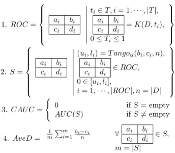
In this paper we analyse three different techniques to establish an optimal-cost class threshold when training data is not available. One technique is directly derived from the definition of cost, a second one is derived from a ranking of estimated probabilities and the third one is based on ROC analysis. We analyse the approaches theoretically and experimentally, applied to the adaptation of existing models. The results show that the techniques we present are better for reducing the overall cost than the classical approaches (e.g. oversampling) and show that cost contextualisation can be performed with good results when no data is available.

1. Introduction

The traditional solution to the problem of contextualising a classifier to a new cost is ROC analysis. In order to perform ROC analysis (as well as other techniques), we need a training or validation dataset, from which we draw the ROC curve in the ROC space. In some situations, however, we don't have any training or validation data analysis available.

This situation is frequent when we have to adapt an existing method which was elaborated by a human expert, or the model is so old that we do not have the old training data used for constructing the initial model available. This is a typical situation in many areas such as engineering, diagnosis, manufacturing, medicine, business, etc. —————

Therefore, the techniques from machine learning or data mining, although they are more and more useful and frequent in knowledge acquisition, cannot be applied if we have models that we want to adapt or to transform, but we do not have the original data.

An old technique that can work without training data is the recently called "cost-sensitive learning by example weighting" (Abe et. al., 2004). The methods which follow this philosophy modify the data distribution in order to train a new model which becomes cost-sensitive. The typical approach in this line is stratification (Breiman et. al., 1984; Chan and Stolfo, 1998) by oversampling or undersampling.

An alternative approach is the use of a threshold. A technique that could be adapted when data is not available can be derived from the classical formulas of cost-sensitive learning. It is straightforward to see (see e.g. Elkan, 2001) that the optimal prediction for an example x

in class i is the one that minimises

∑

=

j

i

C

x

|

j

P

i

x

L

(

,

)

(

)

(

,

)

₍₁₎

where P(j|x) is the estimated probability for each class j

given the example x, and C(i,j) is the cell in the cost matrix C which defines the cost of predicting class i when the true class is j. From the previous formula, as we will see, we can establish a direct threshold without having any extra data at hand. In fact, some existing works (Domingos, 1999) have used the previous formula to establish a threshold which generates a model which is cost sensitive.

One of the most adequate ways to establish a class threshold is based on ROC analysis. (Lachiche & Flach, 2003) extend the general technique and show that it is also useful when the cost has not changed. However, in these cases we need additional validation data, in order to draw the curves.

In order to tackle the problem that we have described at the beginning (adapting an existing model without data), it would be interesting, then, to analyse some techniques

(18)

which combine the direct threshold estimation based on formula 1 (which ignores any estimated probabilities) and methods which take them into account (either their ranking or their absolute value) in a similar way ROC analysis works, but without data.

In order to adapt the existing models, we use the mimetic technique (Domingos, 1997, 1998; Estruch, Ferri, Hernández & Ramírez, 2003; Blanco, Hernández & Ramírez, 2004) to generate a model which is similar to the initial model (oracle) but contextualised to the new cost. In order to do this, we propose at least six different ways to diminish the global cost of the mimetic model. Three criteria for adapting the classification threshold, as we have mentioned, and several different schemas for the mimetic technique are set out (without counting on the original data). We have centered our study on binary classification problems.

The mimetic method is a technique for converting an incomprehensible model into one simple and comprehensible representation. Basically, it considers the incomprehensible model as an oracle, which is used for labelling an invented dataset. Then, a comprehensible model (for instance, a decision tree) is trained with the invented dataset. The mimetic technique has usually been used for obtaining comprehensible models. However, there is no reason for ignoring it as a cost-sensitive adaptation technique since it is in fact a model transformation technique.

Note that the mimetic technique is a transformation technique which can use any learning technique, since the mimetic model is induced from (invented) data.

Figure 1. The mimetic context.

The mimetic context validation (see Figure 1) that we propose allows us to change the context of the initial model (oracle) so that it becomes sensitive to the new cost.

The main advantages of our proposal are that it does not require a retraining of the initial model with the old data and, hence, it is not necessary to know the original data. The only thing we need from the original data or for the formulation of the problem is to know the maximum and minimum values of its attributes.

From these maximum and minimum values and applying the uniform distribution we can obtain an invented dataset, which is labelled by using the oracle. We can use the cost information in different points: on the invented dataset, on the labelling of the data or on the thresholds. This settles three moments at which the cost information is used (see Figure 1, the points Mim1, Mim2 and Mim3). One of the points (Mim2) is especially interesting from the rest because it generates a “specific rule formulation” for the model, which might serve as any explanation of the adaptation to the new costs.

The paper is organised as follows. In section 2 we describe the three methods to determine the thresholds and analyse theoretically the relationships between them. In section 3 we describe the four styles for the generation of invented data and, the schemes used in this work for the learning of the mimetic models. In section 4 we describe the different configurations. We also include the experimental evaluation conducted and the general results, which demonstrate the appropriateness and benefits of our proposal to contextualise any model to a new cost context. Finally, section 5 presents the conclusions and future work.

2. Threshold Estimation

In this section, we present three different methods to estimate an optimal threshold following different philosophies. We also study some theoretical properties of the methods.

In contexts where there are different costs associated to the misclassification errors, or where the class distributions are not identical, a usual way of reducing costs (apart from oversampling) is to find an optimal decision threshold in order to classify new instances according to their associated cost. Traditionally, the way in which the threshold is determined is performed in a simple way (Elkan, 2001), only taking the context skew

into account.

As we have said in the introduction, the methods based on ROC analysis (e.g. Lachiche & Flach, 2003) require a validation dataset, which is created at the expense of reducing data in the training dataset. Here, we are only interested in threshold estimation methods that don’t require extra data, since we do not have any data available (either old or new training or test). Therefore, we will not study this method or others which are related which require a dataset. We will just present methods which can work without it.

Expert D Invented Data Data Mining Technique Ω Semiautomatic Technique Initial Context Ω New Context Dl Labeled Data Learning Algorithm µ Oracle Mimetic

Costs matrix and distribution changes

Mim3 Mim1

Mim2

Context Application

(19)

In this section we consider two-class problems, with class names 0 and 1. Given a cost matrix C, we define the cost

skew as: ) 0 , 0 ( ) 0 , 1 ( ) 1 , 1 ( ) 1 , 0 ( C C C C skew − − = (2) 2.1 Direct Threshold

The first method to obtain the threshold completely ignores the estimated probabilities of the models, i.e., to estimate the threshold it only considers the cost skew. According to (Elkan, 2001), the optimal prediction is class 1 if and only if the expected cost of this prediction is lower than or equal to the expected cost of predicting class 0: ) 1 , 0 ( ) 1 ( ) 0 , 0 ( ) 0 ( ) 1 , 1 ( ) 1 ( ) 0 , 1 ( ) 0 ( |x C P |x C P |x C P |x C P ⋅ + ⋅ ≤ ⋅ + ⋅ If p = P(1|x) we have: ) 1 , 0 ( ) 0 , 0 ( ) 1 ( ) 1 , 1 ( ) 0 , 1 ( ) 1 ( −p ⋅C +p⋅C ≤ −p ⋅C +p⋅C

Then, the threshold for making optimal decisions is a probability p* such that:

) 1 , 0 ( * ) 0 , 0 ( *) 1 ( ) 1 , 1 ( * ) 0 , 1 ( *) 1 ( −p ⋅C +p ⋅C = −p ⋅C +p ⋅C

Assuming that C(1,0)>C(0,0) and C(0,1)>C(1,1) (i.e. misclassifications are more expensive than right predictions), we have ) 1 , 1 ( ) 1 , 0 ( ) 0 , 0 ( ) 0 , 1 ( ) 0 , 0 ( ) 0 , 1 ( * C C C C C C p − + − − = skew p + = 1 1 *

Finally, we define the threshold as:

skew skew p Threshold_Dir + = − = 1 * 1 (3)

2.2 Ranking or Sorting Threshold

The previous method for estimating the classification ignores the estimated probabilities in a proper way. This can be a problem for models that do not distribute the estimated probabilities. Imagine a model that only assigns probabilities within the range 0.6-0.7. In this situation, most of the skews will not vary the results of the model. In order to partially avoid this limitation, we propose a new method to estimate the threshold. The idea is to employ the estimated probabilities directly to compute the

threshold. For this purpose, if we have n examples, we rank these examples according to their estimated probabilities of being class 0. We select a point (Pos) between two points (a,b) in this rank such that there are (approximately) n/(skew+1) examples on the left side and (n* skew/(skew+1)) examples on the right side. In this division point we can find the desired threshold. We can illustrate this situation with Figure 2:

Figure 2. Position of the threshold in the sorting method Following this figure, we have

1 1 1 ₊ + − = skew n

Pos , a=Lower(Pos), b=a+1 where Lower computes the integer part of a real number. Then we estimate the threshold as:

frac p p p ThresholdOrd= _a−( _a− _b)⋅ ₍₄₎ where a Pos frac= −

In the case we find more than one example with the same estimated probability, we distribute these examples in a similar way. A complete explanation of the procedure can be found in (Blanco, 2006).

2.3 ROC Threshold

Although the previous method considers the skew and the estimated probabilities to compute the threshold, it has an important problem because the value of the threshold is restricted to the range of the probabilities computed by the model. I.e, if a model always computes probability estimates between 0.4 and 0.5, the threshold will be within this range for any skew.

Motivated by this limitation, we have studied a new method to compute the threshold based on ROC analysis. Suppose that a model is well calibrated, this fact means that if a model gives a probability 0.8 of being class 0 to 100 examples, 80 should be of class 0, and 20 should be of class 1. In the ROC space, this will be a segment going from point (0,0) to the point (20,80) with a slope of 4. In order to compute this new threshold we define a version of the ROC curve named NROC. This new curve is based on the idea that a probability represents a percentage of correctly classified instances (calibrated classifier). a b ThresholdOrd frac 1−frac Maximum probability

1/(skew+1) skew/(skew+1)

1 n … … pa −pb Pos Index: Minimum Probability pa pb

(20)

If we have a set of n examples ranked by the estimated probability of being class 0, we define Sum0_{as the sum of}

these probabilities. We consider normalised probabilities, then Sum0₊_Sum1₌_n_{. The space NROC is a 2 dimension}

square limited by (0,0) and (1,1). In order to draw a NROC curve, we only take the estimated probabilities into account, and we proceed as follows. If the first example has an estimated probability p1 of being class 0,

we draw a segment from the point (0,0) to the point ((1−p1)/Sum1, p1/Sum0). The next instance (p2) will

correspond to the second segment will be from ((1−p1)/Sum1,p1/Sum0) to (((1−p1)+(1−p2))/Sum1,

((p1+p2)/Sum0). Following this procedure, the last segment

will be between the points (Sum1₋₍₁₋_p

n))/Sum1,

(Sum0_−p

n)/Sum0) and (1,1).

Once we have defined the NROC space, let us explain how we use it to determine the threshold. First, since we work on a normalised ROC space (1×1) and Sum0_{is not}

always equal to Sum1_{, we need to normalise the}_skew_.

1 0 ' Sum Sum skew skew= ⋅

If skew’ is exactly parallel to a segment, then the threshold must be exactly the probability that corresponds to that segment, i.e if skew’=pi/(1−pi) the threshold must

be pi. This means: ' 1 ' skew skew ThresholdROC + =

Using the relationship between skew’ and skew:

1 0 1 0 1 Sum Sum skew Sum Sum skew ThresholdROC ⋅ + ⋅ = 1 0 1 1 1 Sum Sum skew ThresholdROC ⋅ + = (5)

2.4 Theoretical analysis of the threshold methods

Now, we study some properties of the methods for obtaining the threshold which we have described in the previous subsections. First, we show that the threshold which is calculated by each of the three methods is well-defined, that is, it is a real value between 0 and 1, as expected. Secondly, we analyse which the relationship between the three thresholds is.

The maximum and minimum values of the ThresholdDir

and ThresholdROC depend on the skew by definition

(formulae 3 and 5). Trivially, ThresholdOrd belongs to the

interval [0..1] since it is defined as a value between two example probabilities.

Maximum: For the direct and the ROC methods, the maximum is obtained when skew=∞:

1 1 lim lim = + = ∞ → ∞ → skew skew Threshold skew Dir skew 1 1 1 1 lim lim 1 0 = ⋅ + = ∞ → ∞ → Sum Sum skew Threshold skew ROC skew

The upper limit of ThresholdOrd is not necessarily 1, since

it is given by the example with highest probability.

Minimum: For the direct and the ROC methods, the minimum is obtained when skew=0:

0 1 lim lim 0 0 = → + = → skew skew Threshold skew Dir skew 0 1 1 1 lim lim 1 0 0 0 = ⋅ + = → → Sum Sum skew Threshold skew ROC skew

As in the previous case, the lower limit of ThresholdOrd is

not necessarily 0, since it is given by the example with lowest probability.

Regarding the relationship among the three threshold methods, it is clear that we can found cases for which

ThresholdDir > ThresholdOrd, and viceversa, because, as

we have just said, the ThresholdOrd value depends on the

example probability of being of class 0. A similar relationship holds between ThresholdROC and

ThresholdOrd.

However, the relationship between ThresholdROC and

ThresholdDir depends on the relationship between Sum1

and Sum0, as the following proposition shows:

Proposition 2. Given n examples, let Sum0_{be the sum of}

the n (normalised) example probabilities of being in class

0, and let Sum1 _be ₁_−Sum0

. If Sum0/Sum1 > 1 then

ThresholdROC > ThresholdDir, if Sum0/Sum1 < 1 then

ThresholdROC < ThresholdDir, and if Sum0/Sum1= 1 then

ThresholdROC= ThresholdDir .

The following theorem shows that the three thresholds coincide when the probabilities are uniformly distributed. .Proposition 3. Given a set of n examples whose probabilities are uniformly distributed. Let P0_{be the}

sequence of these probabilities ranked downwardly:

} 0 , 1 , 2 ,..., 1 , 1 { 0 m m m m P = −

(21)

such that the probability of example i being in class 0 and class 1 are given respectively by

m i p y m i m p_i0 ₌ − +1 _i1₌ −1 where m=n−1.

Then, ThresholdROC=ThresholdDir=ThresholdOrd. 3. Mimetic Context

In this section we present the mimetic models we will study experimentally in the next section along with the threshold estimation seen in Section 2. For this purpose, we first introduce several ways to generate the invented dataset, as well as different learning schemes. Then, each configuration to be considered will be obtained by inventing its training dataset in a certain way, by applying one of the learning schemes and by using one of the thresholds defined in the previous section.

3.1 Generation of the training dataset for the mimetic technique

As we said in the introduction, we are assuming that the original dataset used for training the oracle is not available. Hence, the mimetic model is training by using only an invented dataset (labelled by the oracle) which is generated using the uniform distribution. This is a very simple approach, because in very few cases data follow this distribution. If we could know the a priori distribution of the data or we could have a sample where we could estimate this distribution, the results would be probably better. Note that, in this way we only need to make use of the range value of each attribute (that is, its maximum and minimum values).

In general, the invented dataset D can be generated by applying one of the following methods:

• Type a: A priori method. In this method, D preserves the class distribution of the original training dataset. To do this, the original class proportion has to be known at the time of the data generation.

• Type b: Balanced method. The same number of examples of each class is generated by this method. So

D is composed by a 50% of examples of class 1 and a 50% of examples of class 0.

• Type c: Random method. The invented dataset D is obtained by only using the uniform distribution as it is (that is, no conditions about the class frequency in D

are imposed).

• Type d: Oversampling method. This method makes that the class frequencies in the invented dataset are defined in terms of the skew, such that D contains a proportion of 1/(skew+1) of instances of class 0 and a proportion of skew/(skew+1) of instances of class 1.

In order to obtain the four types, we generate random examples and then we label them using the oracle. This process is finished when we obtain the correct percentage according to the selected type.

3.2 Mimetic Learning Schemes

In order to use the mimetic approach for a context sensitive learning, different mimetic learning schemes can be defined depending on the step of the mimetic process the context information is used: at the time of generating the invented dataset (scheme 3), at the time of labelling the invented dataset (scheme 1) or at the time of application of the mimetic model (scheme 2). We also consider another scheme (scheme 0) which corresponds to the situation where the context information is not used (as a reference). More specifically, we define the following mimetic learning schemes:

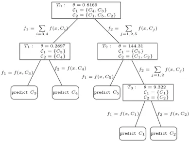
• Scheme 0 (Mim0 model): This is the basic mimetic scheme. The mimetic model is obtained by applying a decision tree learner to the labelled data, namely the J48 classifier with pruning (Figure 3). Then, Mim0 is applied as a non sensitive context model that classifies a new example of class 0 if the probability for this class is greater or equal to 0.5 (threshold=0.5).

Figure 3. Scheme 0: The simple mimetic learning method.

• Scheme 1 (Mim1 model): This is a posteriori scheme in that the context information is used when the mimetic model is applied. First, the mimetic model is obtained as usually (by using the J48 classifier without pruning). Then, the threshold is calculated from the mimetic model and the invented dataset. Finally, the Mim1 model uses these parameters to classify new examples. Figure 4 shows this learning scheme.

Figure 4. Scheme 1: The context information is used at the time of the mimetic model application.

• Scheme 2 (Mim2 model): This is a priori scheme in which the context information is used before the mimetic model is learned. Once the invented dataset has been labelled by the oracle, the threshold and the Ro index (if it is needed) are calculated from them. Then, the invented dataset is re-labelled using these parameters. The new dataset is used for training the mimetic model which is applied as in scheme 0. This learning scheme is very similar to the proposal of

J48 without pruning D Dl Apply using T Threshold T Calculation Ω Mimetic model µ Selection J48 with pruning

D _Ω Dl µ Apply using Threshold=0,5 Selection

Oracle Mimetic model