9HSTF
MG*aea
fcd+
ISBN: 978-952-60-4053-0 (pdf) ISBN: 978-952-60-4052-3 ISSN-L: 1799-4934 ISSN: 1799-4942 (pdf) ISSN: 1799-4934 Aalto University School of EconomicsDepartment of Business Technology aalto.fi BUSINESS + ECONOMY ART + DESIGN + ARCHITECTURE SCIENCE + TECHNOLOGY CROSSOVER A alt o-D D 1 7 /2 01 1 An ku r S in ha Pr og re ssi ve ly I nte ra cti ve E vo lu tio na ry M ult io bje cti ve O pti m iza tio n A alt o U n iv e
Department of Business Technology
Progressively
Interactive
Evolutionary
Multiobjective
Optimization
Ankur Sinha
Aalto University publication series
DOCTORAL DISSERTATIONS 17/2011
Progressively Interactive Evolutionary
Multiobjective Optimization
Ankur Sinha
Aalto University publication series DOCTORAL DISSERTATIONS 17/2011 © Ankur Sinha ISBN 978-952-60-4053-0 (pdf) ISBN 978-952-60-4052-3 (printed) ISSN-L 1799-4934 ISSN 1799-4942 (pdf) ISSN 1799-4934 (printed)
Abstract
Aalto University, P.O. Box 11000, FI-00076 Aalto www.aalto.fi
Author Ankur Sinha
Name of the doctoral dissertation
Progressively Interactive Evolutionary Multiobjective Optimization Publisher Aalto University School of Economics
Unit Department of Business Technology
Series Aalto University publication series DOCTORAL DISSERTATIONS 17/2011 Field of research Decision Making and Optimization
Abstract
A complete optimization procedure for a multi-objective problem essentially comprises of search and decision making. Depending upon how the search and decision making task is integrated, algorithms can be classified into various categories. Following `a decision making after search' approach, which is common with evolutionary multi-objective optimization algorithms, requires to produce all the possible alternatives before a decision can be taken. This, with the intricacies involved in producing the entire Pareto-front, is not a wise approach for high objective problems. Rather, for such kind of problems, the most preferred point on the front should be the target. In this study we propose and evaluate algorithms where search and decision making tasks work in tandem and the most preferred solution is the outcome. For the two tasks to work simultaneously, an interaction of the decision maker with the algorithm is necessary, therefore, preference information from the decision maker is accepted periodically by the algorithm and progress towards the most preferred point is made.
Two different progressively interactive procedures have been suggested in the dissertation which can be integrated with any existing evolutionary multi-objective optimization algorithm to improve its effectiveness in handling high objective problems by making it capable to accept preference information at the intermediate steps of the algorithm. A number of high objective un-constrained as well as constrained problems have been successfully solved using the procedures. One of the less explored and difficult domains, i.e., bilevel multi-objective optimization has also been targeted and a solution methodology has been proposed. Initially, the bilevel multi-objective optimization problem has been solved by developing a hybrid bilevel evolutionary multi-objective optimization algorithm. Thereafter, the progressively interactive procedure has been incorporated in the algorithm leading to an increased accuracy and savings in computational cost. The efficacy of using a progressively interactive approach for solving difficult multi-objective problems has, therefore, further been justified.
Keywords Evolutionary multi-objective optimization algorithms, multiple criteria decision-making, interactive multi-objective optimization algorithms, bilevel optimization ISBN (printed) 978-952-60-4052-3 ISBN (pdf) 978-952-60-4053-0
Progressively Interactive Evolutionary Multi-objective
Optimization
Ankur Sinha
Department of Business Technology
P.O. Box 21210, FI-00076
Aalto University School of Economics
Helsinki, Finland
[email protected]
Abstract
A complete optimization procedure for a multi-objective problem
essen-tially comprises of search and decision making. Depending upon how the
search and decision making task is integrated, algorithms can be
classi-fied into various categories. Following ‘a decision making after search’
approach, which is common with evolutionary multi-objective
optimiza-tion algorithms, requires to produce all the possible alternatives before a
decision can be taken. This, with the intricacies involved in producing
the entire Pareto-front, is not a wise approach for high objective problems.
Rather, for such kind of problems, the most preferred point on the front
should be the target. In this study we propose and evaluate algorithms
where search and decision making tasks work in tandem and the most
preferred solution is the outcome. For the two tasks to work
simultane-ously, an interaction of the decision maker with the algorithm is necessary,
therefore, preference information from the decision maker is accepted
pe-riodically by the algorithm and progress towards the most preferred point
is made.
Two different progressively interactive procedures have been suggested
in the dissertation which can be integrated with any existing
evolution-ary multi-objective optimization algorithm to improve its effectiveness in
handling high objective problems by making it capable to accept
prefer-ence information at the intermediate steps of the algorithm. A number of
high objective un-constrained as well as constrained problems have been
successfully solved using the procedures. One of the less explored and
difficult domains, i.e., bilevel multi-objective optimization has also been
targeted and a solution methodology has been proposed. Initially, the
bilevel multi-objective optimization problem has been solved by
develop-ing a hybrid bilevel evolutionary multi-objective optimization algorithm.
Thereafter, the progressively interactive procedure has been incorporated
in the algorithm leading to an increased accuracy and savings in
compu-tational cost. The efficacy of using a progressively interactive approach
for solving difficult multi-objective problems has, therefore, further been
justified.
General Keywords
: Evolutionary multi-objective optimization algorithms,
multiple criteria decision-making, interactive multi-objective optimization
algorithms, bilevel optimization
Additional Keywords
: Preference based multi-objective optimization,
hy-brid evolutionary algorithms, self-adaptive algorithm, sequential quadratic
programming, algorithm development, test problem development
Acknowledgements
The dissertation has been completed at the Department of Business
Tech-nology, Aalto University School of Economics. The work has been
per-formed under the supervision of Prof. Kalyanmoy Deb, Prof. Pekka
Ko-rhonen and Prof. Jyrki Wallenius. I would like to extend heartfelt
grati-tude and thanks to my supervisors for their inspiration and support which
motivated me to start working on the dissertation with utmost enthusiasm
and has been the driving force for successfully accomplishing the task.
Their constant support and fruitful discussions encouraged new thoughts
and ideas which were instrumental in executing the work. I consider
my-self fortunate to receive the best possible guidance and mentoring from
the leading researchers in the field of Evolutionary Multi-objective
Opti-mization and Multi Criteria Decision Making.
I thank the pre-examiners of this thesis, Prof. Juergen Branke and Prof.
Lothar Thiele for their valuable feedback that helped in improving the
dis-sertation. I would also thank all my colleagues at the department, in
par-ticular, Antti Saastamoinen, Pekka Malo and Oskar Ahlgren for providing
a friendly work environment. I express my gratitude to the the
depart-ment secretaries, Helena Knuuttila, Merja M¨akinen and Jutta Heino for
their unconditional help and support.
I gracefully thank the graduate school on ‘Systems Analysis, Decision
Making and Risk Management’, HSE foundation and the Academy of
Fin-land for financially supporting this study. I would like to dedicate this
the-sis to my parents as I could not have accomplished the task successfully
without their blessings. Finally, I wish to give a special mention to my
wife, Parul, whose love, affection and support kept me rejuvenated even
towards the completion of my dissertation.
Contents
I
Overview of the Dissertation
1
1
Introduction
3
1.1
Multi-objective Optimization . . . .
4
1.2
Domination Concept and Optimality . . . .
5
1.2.1
Domination Concept . . . .
5
1.3
Decision Making . . . .
8
1.4
Evolutionary Multi-objective Optimization (EMO) Algorithms 10
1.5
Integrating Search and Decision Making . . . 12
1.5.1
A posteriori Approach . . . 12
1.5.2
A priori Approach . . . 14
1.5.3
Interactive Approach . . . 15
1.6
Motivation . . . 17
1.7
Summary of Research Papers . . . 18
1.7.1
An Interactive Evolutionary Multi-Objective
Opti-mization Method Based on Progressively
Approxi-mated Value Functions . . . 19
1.7.2
Progressively Interactive Evolutionary Multi-Objective
Optimization Method Using Generalized Polynomial
Value Functions . . . 19
1.7.3
An Interactive Evolutionary Multi-Objective
Opti-mization Method Based on Polyhedral Cones . . . . 20
1.7.4
An Efficient and Accurate Solution Methodology for
Bilevel Multi-Objective Programming Problems
Us-ing a Hybrid Evolutionary-Local-Search Algorithm . 20
1.7.5
Bilevel Multi-Objective Optimization Problem
Solv-ing UsSolv-ing Progressively Interactive EMO . . . 21
II
List of Papers
27
1
An interactive evolutionary multi-objective optimization method
based on progressively approximated value functions
K. Deb, A. Sinha, P. Korhonen, and J. Wallenius
IEEE Transactions on Evolutionary Computation, 14(5), 723-739.
IEEE Press, 2010.
29
2
Progressively interactive evolutionary multi-objective
optimiza-tion method using generalized polynomial value funcoptimiza-tions
A. Sinha, K. Deb, P. Korhonen, and J. Wallenius
In Proceedings of the 2010 IEEE Congress on Evolutionary
Compu-tation (CEC-2010), pages 1-8. IEEE Press, 2010.
47
3
An interactive evolutionary multi-objective optimization method
based on polyhedral cones
A. Sinha, P. Korhonen, J. Wallenius, and K. Deb
In Proceedings of the 2010 Learning and Intelligent Optimization
Conference (LION-2010), pages 318-332. IEEE Press, 2010.
57
4
An efficient and accurate solution methodology for bilevel
multi-objective programming problems using a hybrid
evolutionary-local-search algorithm
K. Deb and A. Sinha
Evolutionary Computation Journal, 18(3), 403-449. MIT Press, 2010. 73
5
Bilevel multi-objective optimization problem solving using
pro-gressively interactive EMO
A. Sinha
In Proceedings of the Sixth International Conference on
Part I
1
Introduction
Many real-world applications of multi-objective optimization involve a
high number of objectives. Existing evolutionary multi-objective
opti-mization algorithms [7, 34] have been applied to problems having
mul-tiple objectives for the task of finding a well-representative set of
Pareto-optimal solutions [6, 4]. These methods have been successful in solving a
wide variety of problems with two or three objectives. However, these
methodologies tend to fail for high number of objectives (greater than
three) [8, 22]. The major hindrances in handling high number of objectives
relate to stagnation in search, increased dimensionality of Pareto-optimal
front, large computational cost, and difficulty in visualization of the
ob-jective space. These difficulties are inherent to a multi-obob-jective problem
having a high number of dimensions and cannot be eliminated; rather,
procedures to handle such difficulties need to be explored.
In many of the existing methodologies, preference information from
the decision maker is utilized before the beginning of the search process
or at the end of the search process to produce the optimal solution(s) in
a multi-objective problem. Some approaches interact with the decision
maker and iterate the process of elicitation and search until a satisfactory
solution is found. However, not many studies have been performed where
preference information is elicited during the search process and the
infor-mation is utilized to progressively proceed towards the most preferred
solution.
This dissertation is an effort towards development of progressively
in-teractive procedures to handle difficult multi-objective problems,
combin-ing concepts from the fields of Evolutionary Multi-objective Optimization
(EMO) and Multi Criteria Decision Making (MCDM). The fields of
Evolu-tionary Multi-objective Optimization and Multi Criteria Decision Making
have a common goal, but researchers have shown only lukewarm
inter-est, until recently, in applying the principles of one field to the other. In
the dissertation, emphasis has been placed on integration of methods and
development of hybrid procedures that are helpful in the extension of the
existing algorithms to handle challenging problems with multiple
objec-tives. The utility of the procedures has also been shown on bilevel
multi-objective optimization problems. The amalgamation of ideas has
pro-found ramifications and addresses the challenges posed by multi-objective
optimization problems.
The dissertation is composed of five papers which have been
summa-rized in this introductory chapter. Before providing a summary, a short
review of the basic concepts necessary to understand the papers will be
given in the following sections.
1.1
Multi-objective Optimization
In a multi-objective optimization problem [30, 19, 6] there are two or more
conflicting objectives which are supposed to be simultaneously optimized
subject to a given set of constraints. These problems are commonly found
in the fields of science, engineering, economics or any other field where
optimal decisions are to be taken in the presence of trade-offs between
two or more conflicting objectives. Usually such problems do not have a
single solution which would simultaneously maximize/minimize each of
the objectives; instead, there is a set of solutions which are optimal. These
optimal solutions are called the Pareto-optimal solutions. A general
multi-objective problem (
M
≥
2
) can be described as follows:
Maximize
f
(
x
) = (f
1(
x
), . . . , f
M(
x
))
,
subject to
g
(
x
)
≥
0
,
h
(
x
) =
0
,
x
(iL)≤
x
i≤
x
(iU),
i
= 1, . . . , n.
(1.1)
In the above formulation,
x
represents the decision variable which lies
in the decision space. The decision space is the search space represented
by the constraints and variable bounds in a general multi-objective
prob-lem statement. The objective space
f
(
x
)
is the image of the decision space
under the objective function
f
. In a single objective optimization (
M
= 1
)
problem the feasible set is completely ordered according to the objective
function
f
(
x
) =
f
1(
x
)
, such that for solutions,
x
(1)and
x
(2)in the decision
space, either
f
1(
x
(1))
≥
f
1(
x
(2))
or
f
1(
x
(2))
≥
f
1(
x
(1))
. Therefore, for two
solutions in the objective space there are two possibilities with respect to
the
≥
relation.
However, when several objectives (
M
≥
2
) are involved, the feasible
set is not necessarily completely ordered, but partially ordered. In
multi-objective problems, for any two multi-objective vectors,
f
(
x
(1))
and
f
(
x
(2))
, the
relations
=
,
>
and
≥
can be extended as follows,
•
f
(
x
(1))
≥
f
(
x
(2))
f
i
(
x
(1))
≥
f
i(
x
(2))
:
⇔
i
∈ {
1,
2, . . . , M
}
•
f
(
x
(1))
>
f
(
x
(2))
⇔
f
(
x
(1))
≥
f
(
x
(2))
∧
f
(
x
(1))
6
=
f
(
x
(2))
While comparing the multi-objective scenario with the single objective
case [5], in contrast we find that for two solutions in the objective space
there are three possibilities with respect to the
≥
relation. These
possibili-ties are:
f
(
x
(1))
≥
f
(
x
(2))
,
f
(
x
(2))
≥
f
(
x
(1))
or
f
(
x
(1))
f
(
x
(2))
∧
f
(
x
(2))
f
(
x
(1))
. If any of the first two possibilities are met, it allows to rank or
order the solutions independent of any preference information (or a
deci-sion maker). On the other hand, if the first two possibilities are not met,
the solutions cannot be ranked or ordered without incorporating
prefer-ence information (or involving a decision maker). Drawing analogy from
the above discussion, the relations
<
and
≤
can be extended in a similar
way.
1.2
Domination Concept and Optimality
1.2.1
Domination Concept
Based on the established binary relations for two vectors in the previous
section, the following domination concept [14] can be constituted,
•
x
(1)strongly dominates
x
(2)⇔
f
(
x
(1))
>
f
(
x
(2))
,
•
x
(1)weakly dominates
x
(2)⇔
f
(
x
(1))
≥
f
(
x
(2))
,
•
x
(1)and
x
(2)are non-dominated with respect to each other
⇔
f
(
x
(1))
f
(
x
(2))
∧
f
(
x
(2))
f
(
x
(1))
.
The above domination concept is also explained in Figure 1.1 for a two
objective maximization case. In Figure 1.1 two shaded regions have been
shown in reference to point A. The shaded region in the north-east corner
(excluding the lines) is the region which strongly dominates point A, the
shaded region in the south-west corner (excluding the lines) is strongly
dominated by point A and the unshaded region is the non-dominated
re-gion. Therefore, point A strongly dominates point B, points A, E and D are
non-dominated with respect to each other, and point A weakly dominates
point C.
Most of the existing evolutionary multi-objective optimization
algo-rithms use the domination principle to converge towards the optimal set
of solutions. The concept allows us to order two decision vectors based
on the corresponding objective vectors in the absence of any preference
A f2 f1 D C B E Dominated by A Region Dominating A Region
Figure 1.1:
Explanation for
the domination concept for a
maximization problem where A
strongly dominates B; A weakly
dominates C; A, D and E are
non-dominated.
1 2 3 4 2 5 f2 f1 Pareto−optimal Front Non−dominated Set 4 2 1 5 3indifference incomparable preference
Figure 1.2: Explanation for the
concept of a non-dominated set
and a Pareto-optimal front. A
hy-pothetical decision maker’s
pref-erences for binary pairs are also
shown.
information. The algorithms which operate with a sparse set of solutions
in the decision space and the corresponding images in the objective space
usually give priority to a solution which dominates another solution. The
solution which is not dominated with respect to any other solution in the
sparse set is referred to as a non-dominated solution.
In case of a discrete set of solutions: the subset whose solutions are
not dominated by any solution in the discrete set is referred to as the
non-dominated set within the discrete set. The non-dominated set consists
of the best solutions available and form a front called a non-dominated
front. When the set in consideration is the entire search space, the
result-ing non-dominated set is referred as a Pareto-optimal set and the front is
referred as the Pareto-optimal front. To formally define a Pareto-optimal
set, consider a set
X
, which constitutes the entire decision space with
so-lutions
x
∈
X
. The subset
X
∗:
X
∗⊂
X
, containing solutions
x
∗, which
are not dominated by any
x
in the entire decision space forms a
Pareto-optimal set.
The concept of a Pareto-optimal front and a non-dominated front are
illustrated in Figure 1.2. The shaded region in the figure represents
f
(
x
) :
x
∈
X
. It is the image in the objective space of the entire feasible region
in the decision space. The bold curve represents the Pareto-optimal front
for a maximization problem. Mathematically, this curve is
f
(
x
∗) :
x
∗∈
X
∗which are all the optimal points for the two objective optimization
prob-lem. A number of points are also plotted in the figure, which constitute
a finite set. Among this set of points, the points connected by broken
lines are the points which are not dominated by any point in the finite
set. Therefore, these points constitute a non-dominated set within the
fi-nite set. The other points which do not belong to the non-dominated set
are dominated by at least one of the points in the non-dominated set.
In the field of Multi-Criteria Decision Making, the terminology slightly
differs. For a given set of points in the objective space, the points which
are not dominated by any other point belonging to the set are referred
as non-dominated points, and their corresponding images in the decision
space are referred as efficient. Based on the definition of weak and strong
domination for a pair of points, the concept of weak efficiency and strong
efficiency can be developed for a point within a set. A point
x
∗∈
X
, is
weakly efficient if and only if there does not exist another
x
∈
X
such
that
f
i(
x
)
> f
i(
x
∗)
for
i
∈ {
1,
2, . . . , M
}
. Weak efficiency should be
dis-tinguished from strong efficiency which states that a point
x
∗∈
X
, is
strongly efficient if and only if there does not exist another
x
∈
X
such
that
f
i(
x
)
≥
f
i(
x
∗)
for all
i
and
f
i(
x
)
> f
i(
x
∗)
for at least one
i
.
The terminologies, efficiency and non-domination, are used differently
in different fields. The researchers in the field of Data Envelopment
Anal-ysis tend to call the points in the objective space as efficient or inefficient.
Some researchers prefer to call only the pareto-optimal points as efficient
or non-dominated points. To avoid any confusion, we shall not be
differ-entiating between efficiency and non-domination and the terminologies
will be used only in reference to points belonging to a set. The two
ter-minologies will be used synonymously for points in the objective space as
well as the decision space, based on domination comparisons performed
in the objective space. If the set in which domination comparisons are
made, encompasses the entire feasible region in the objective space, then
the efficient or non-dominated points for that set will be referred as
pareto-optimal points.
In Figure 1.3, for a set of points
{
1,
2,
3,
4,
5,
6,
7,
8,
9,
10
}
, the points
{
1,
2,
3,
4,
5,
6,
7,
8,
9
}
are weakly efficient and the points
{
1,
2,
3,
4,
5
}
are
strongly efficient. Note that the set of all strongly efficient points is a
sub-set of the sub-set of all weakly efficient points. The point
{
10
}
is inefficient as
it is dominated by at least one other point in the set. It should be noted
that the notion of efficiency arises while comparing points within a set.
Here the set in consideration consists of 10 number of points with few as
f2 f1 Inefficient C Efficient Strongly 9 8 5 4 3 2 1 7 6 A B D 10
Figure 1.3: Explanation for efficiency
strongly efficient. The efficient points are not necessarily Pareto-optimal
as it is obvious from the figure. The frontier ABCD represented in the
fig-ure is a weak Pareto-frontier and the subset BC shown in bold is a strong
Pareto-frontier.
1.3
Decision Making
Even though there are multiple optimal solutions to a multi-objective
prob-lem, there is often just a single solution which is of interest to the decision
maker; this is termed as the most preferred solution. Search and decision
making are two intricacies [18] involved in handling any multi-objective
problem. Search requires an intensive exploration in the decision space to
get close to the optimal solutions; on the other hand, decision making is
re-quired to provide preference information for the non-dominated solutions
in pursuance of the most preferred solution.
In a decision making context the solutions can be compared and
or-dered based on the preference information, though there can be situations
where strict preference of one solution over the other is not obtained and
the ordering is partial. For instance, consider two vectors,
x
(1)and
x
(2), in
the decision space having their images,
f
(
x
(1))
and
f
(
x
(2))
, in the objective
space. A preference structure can be defined using three binary relations
,
∼
and
k
,
•
x
(1)∼
x
(2)⇔
x
(1)and
x
(2)are equally preferable,
•
x
(1)k
x
(2)⇔
x
(1)and
x
(2)are incomparable,
where the preference relation,
, is asymmetric, the indifference relation,
∼
, is reflexive and symmetric and the incomparability relation,
k
, is
ir-reflexive and symmetric. A weak preference
relation can be established
as
=
∪ ∼
such that,
•
x
(1)x
(2)⇔
x
(1)is either preferred over
x
(2)or they are equally
preferred.
As already mentioned, preference can easily be established for pairs
where one solution dominates the other. However, for pairs which are
non-dominated with respect to each other, a decision is required to
estab-lish a preference. The following are the inferences for preference choice
which can be drawn from dominance:
•
If
x
(1)strongly dominates
x
(2)⇒
x
(1)x
(2),
•
If
x
(1)weakly dominates
x
(2)⇒
x
(1)x
(2).
The binary relations
,
∼
and
k
, are also explained in Figure 1.2 for
a two objective case. Multiple points have been shown in the objective
space and when comparisons are made between solutions in pairs then
one of the binary relations will hold. For example, points 1 and 2 are close
to each other; therefore, a decision maker may be indifferent between the
two points. Points 3 and 4 lie on the extremes and are far away from
each other; therefore, a decision maker may find such points
incompara-ble. When points 2 and 5 are considered, a decision maker is not required
as 2 dominates point 5; it can be directly inferred that a rational decision
maker will prefer 2 over 5.
It is common to emulate a decision maker with an non-decreasing
value function,
V
(
f
(
x
)) =
V
(f
1(
x
), . . . , f
M(
x
))
, which is scalar in nature
and assigns a value or a measure of satisfaction to each of the solution
points. For two solutions,
x
(1)and
x
(2),
•
If
x
(1)x
(2)⇔
V
(
f
(
x
(1)))
> V
(
f
(
x
(2)))
,
1.4
Evolutionary Multi-objective Optimization (EMO)
Algorithms
An evolutionary algorithm is a generic population based optimization
al-gorithm which uses a mechanism inspired by biological evolution, i.e.,
selection, mutation, crossover and replacement. The common
underly-ing idea behind an evolutionary technique is that, for a given
popula-tion of individuals, the environmental pressure causes natural selecpopula-tion
which leads to a rise in fitness of the population. A comprehensive
dis-cussion of the principles of an evolutionary algorithm can by found in
[16, 24, 12, 1, 25]. In contrast to classical algorithms which iterate from
one solution point to the other until termination, an evolutionary
algo-rithm works with a population of solution points. Each iteration of an
evolutionary algorithm results in an update of the previous population by
eliminating inferior solution points and including the superior ones. In
the terminology of evolutionary algorithms an iteration is commonly
re-ferred to as a generation and a solution point as an individual. A pseudo
code for a generic evolutionary algorithm is provided next:
Step 1: Create a random initial population
Step 2: Evaluate the individuals in the population and assign fitness
Step 3: Repeat the generations until termination
Sub-step 1: Select the most fit individuals (parents) from the
popu-lation for reproduction
Sub-step 2: Produce new individuals (offsprings) through Crossover
and Mutation operators
Sub-step 3: Evaluate the new individuals and assign fitness
Sub-step 4: Replace low fitness members with high fitness members
in the population
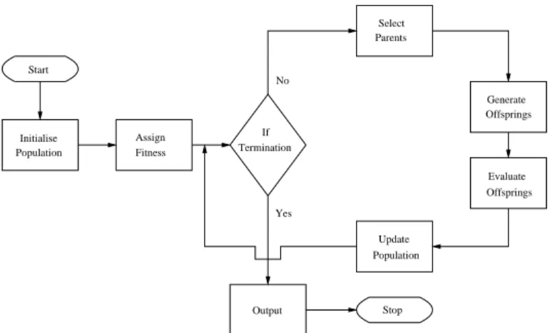
Step 4: Output
Along with the pseudo code presented above, a flowchart for a general
evolutionary algorithm has also been presented in Figure 1.4. A pool of
individuals is generated by randomly creating points in the search space
which is called the population. Each member in the population is
evalu-ated and assigned a fitness. For instance, while solving a single objective
Population Initialise Fitness Assign Termination Select Parents Update Population Output Start Stop If No Yes Offsprings Evaluate Generate Offsprings
Figure 1.4: A flowchart for a general evolutionary algorithm
maximization problem, a solution point with a higher function value is
better than a solution point with lower function value. Therefore, in such
cases, the individual with higher function value is assigned a higher
fit-ness. The function value can itself be treated as a fitness value in this case,
or they can be transformed through a quality function to give the fitness
measure. Similarly, for a multi-objective maximization problem a solution
point which dominates another solution point is considered to be better.
There is also a measure for crowdedness [6] which is used for individuals
which cannot be ordered based on the domination principle. A
multi-objective evolutionary procedure, therefore, assigns fitness to each of the
solution points based on their superiority over other solutions points in
terms of domination and crowdedness. Different algorithms use different
approaches to assign fitness to an individual in a population. Once an
ini-tial population is generated and the fitness is assigned, few of the better
candidates from the population are chosen as parents. Crossover and
mu-tation is performed to generate new solutions. Crossover is an operator
applied to two or more selected individuals and results in one or more
new individuals. Mutation is applied to a single individual and results in
one new individual. Executing crossover and mutation leads to offsprings
that compete, based on their fitness, with the individuals in the
popula-tion, for a place in the next generation. An iteration of this process leads
to a rise in the average fitness of the population.
Using the described evolutionary framework, a number of algorithms
have been developed which successfully solve a variety of optimization
problems. Their strength is particularly observable in handling
multi-objective optimization problems and generating the entire Pareto front.
The aim of an evolutionary multi-objective optimization (EMO) algorithm
is to produce solutions which are (ideally) Pareto-optimal and uniformly
distributed over the entire Pareto-front so that a complete representation
is provided. In the domain of EMO algorithms these aims are commonly
referred to as convergence and diversity. The researchers in the EMO
com-munity have so far regarded an a posteriori approach to be an ideal
ap-proach where a representative set of Pareto-optimal solutions are found
and then a decision maker is invited to select the most preferred point.
The assertion is that only a decision maker who is well informed is in a
position to take a right decision. A common belief is that decision
mak-ing should be based on complete knowledge of the available alternatives;
current research in the field of EMO algorithms has taken inspiration from
this belief. Though the belief is true to a certain extent, there are
inher-ent difficulties associated with producing the inher-entire set of alternatives and
performing decision making thereafter, which many a times renders the
approach ineffective.
1.5
Integrating Search and Decision Making
Search and Decision Making can be combined in various ways to generate
procedures which can be classified into three broad categories [19]. Each
of the approaches to integrate the search and decision making will be
dis-cussed in the following sub-sections.
1.5.1
A posteriori Approach
In this approach, after a set of (approximate) Pareto-optimal solutions are
obtained using an optimization algorithm, decision making is performed
to find the most preferred solution. Figure 1.5 shows the process followed
to arrive at the final solution which is most preferred to a decision maker.
This approach is based on the assumption that a complete knowledge of
all the alternatives helps in taking better decisions. The research in the
field of evolutionary multi-objective optimization has been directed along
this approach, where the aim is to produce all the possible alternatives for
the decision maker to make a choice. The community has largely ignored
decision making aspects, and has been striving towards producing all the
possible optimal solutions.
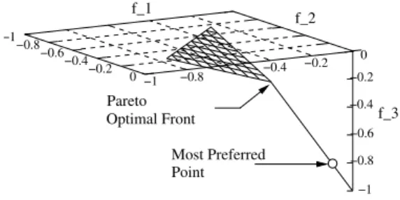
There are enormous difficulties in finding the entire Pareto-optimal
front for a high objective problem. Even if it is assumed than an
algo-rithm can approximate the Pareto-optimal front for a high objective
prob-lem with a huge set of points, the herculean task of choosing the best point
from the set still remains. For two and three objectives where the
solu-tions in the objective space could be represented geometrically, making
decisions might be easy (though even such an instance could be, in reality,
a difficult task for a decision maker). Imagine a multi-objective problem
with more than three objectives for which an evolutionary multi-objective
algorithm is able to produce the entire front. The front is approximated
with high accuracy and high number of points. Since a graphical
represen-tation is not possible for the Pareto-points, how is a decision maker going
to choose the most preferred point? There are of course decision aids
avail-able, but the limited accuracy with which the final choice could be made
using these aids, questions the purpose of producing the entire front with
a high accuracy. Binary comparisons can be a solution to choose the best
point out of a set, but this can only be utilized if the points are very few
in number. Therefore, offering the entire set of Pareto-points should not
be considered as a complete solution to the problem. However, the
diffi-culties related to decision making have been realized by EMO researchers
only after copious research has already gone towards producing the entire
Pareto-front for many objective problems.
Computational Resources Solutions Pareto−optimal Decision Maker Most Preferred Solution Minimize/Maximize F(x) = (f1(x), f2(x))
1.5.2
A priori Approach
In this approach, decision making is performed before the start of the
al-gorithm, then the optimization algorithm is executed by incorporating the
preference rules, and the most preferred solution is identified. Figure 1.6
shows the process followed to arrive at the most preferred solution. This
approach has been common among MCDM practitioners, who realized
the complexities involved in decision making for such problems. Their
ap-proach to the problem is to ask simple questions from the decision maker
before starting the search process. The initial queries usually include the
direction of search, aspiration levels for the objectives, or preference
infor-mation for one or more given pairs. After eliciting such inforinfor-mation from
the decision maker, the multi-objective problem is usually converted into
a single objective problem. One of the early approaches, that is,
Multi-Attribute Utility Theory (MAUT) [21] used the initial information from
the decision maker to construct a utility function which reduced the
prob-lem to a single objective optimization probprob-lem. Scalarizing functions (for
example, [32]) are also commonly used by the researchers in this field to
convert a multi-objective problem into a single objective problem. Other
techniques which are used to elicit information from a decision maker can
be found in the review [23] on multi-criteria decision support.
Since information is elicited towards the beginning, the solution
ob-tained after executing the algorithm is usually a satisfactory solution and
may not be close to the most preferred solution. Moreover, the decision
makers’ preferences might be different for solutions close to the
Pareto-optimal front and the initial inputs taken from them may not confirm it.
Therefore, it will be difficult to get close to the actual solution which
con-firms to the requirements of the decision maker. The approach is also
highly error prone as even slight deviations in providing preference
in-formation at the beginning may lead to entirely different solutions. To
avoid the errors due to deviations, researchers in the EMO field used the
approach in a slightly modified way. They produced multiple solutions in
the region of interest to the decision maker [2, 11, 31, 17], instead of a
sin-gle solution, therefore, giving choices to the decision maker at the end of
the EMO search. However, researchers in the MCDM field recognized the
enormous possibilities which could lead to erroneous results and therefore
there exists a different school of thought which focusses on interactive
ap-proaches.
Decision Maker Computational Resources Most Preferred Solution Minimize/Maximize F(x) = (f1(x), f2(x))
Figure 1.6: A priori approach.
1.5.3
Interactive Approach
In this approach, the decision maker interacts with the optimization
algo-rithm and has multiple opportunities to provide preference information
to the algorithm. The interaction between the decision maker and the
op-timization algorithm continues until a solution acceptable to the decision
maker is obtained. The process is represented in Figure 1.7. Based on the
type of interaction of the decision maker with the optimization algorithm,
a variety of interactive approaches can exist. The dissertation discusses a
special kind of an interactive approach referred as Progressively
Interac-tive Approach.
Progressively Interactive Approach
A progressively interactive approach involves elicitation of preference
in-formation periodically from a decision maker. While the optimization
al-gorithm is underway, preference information is taken at the intermediate
steps of the algorithm, and the algorithm proceeds towards the most
pre-ferred point. This is a more effective integration of the search and decision
making process, as both work simultaneously towards the exploration of
the solution.
This approach overcomes the limitations of the previously discussed
approaches as it allows actual interaction of the decision maker with the
algorithm. The algorithm takes decision maker’s preferences into account
Computational Resources Decision Maker Most Preferred Solution Minimize/Maximize F(x) = (f1(x), f2(x))
Figure 1.7: Interactive approach.
after every small step it takes towards the Pareto-optimal front. The
ap-proach offers a major advantage, as it allows the decision makers to change
their preference structure as the algorithm progresses and more solutions
are explored. Though the algorithm allows the decision maker to be seated
in the driver’s seat and have a greater control over the algorithm, it does
not get mis-directed by a few errors which any human decision maker
is prone to make. A progressively interactive approach with small step
sizes (or frequent elicitation) is guaranteed to take a decision maker very
close to the most preferred solution, as shown in the dissertation. The
dissertation suggests two procedures which use a progressively
interac-tive approach. In the first procedure, the decision maker value function
is approximated after each step, and the second procedure constructs a
polyhedral cone after each step. The progressively interactive approach
is promising, as it avoids the drawbacks present in the other approaches.
Some previous work which has been done in a similar vein in the MCDM
field are [15, 33]. Little work [26, 13, 20, 3] on progressively interactive
ap-proach has been done in the field of EMO and calls for more contributions
from researchers.
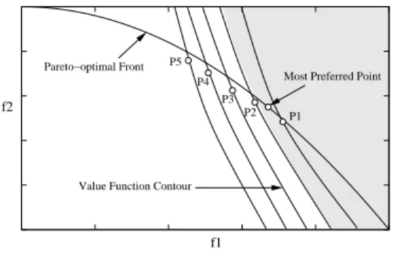
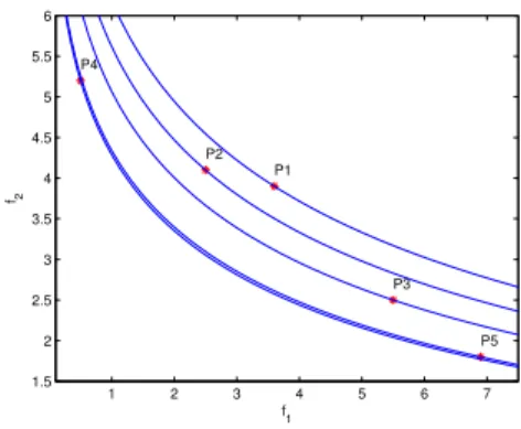
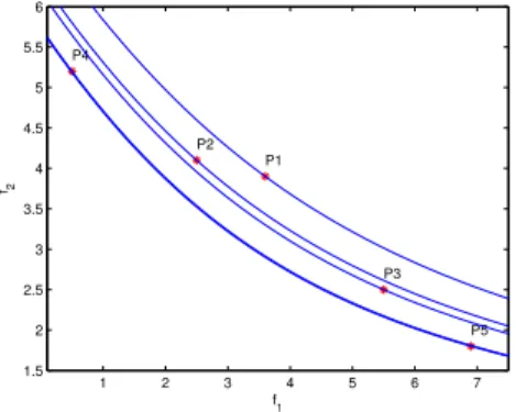
The iterations of a simple algorithm using a progressively interactive
approach has been shown in the Figure 1.8. The decision maker is
pre-sented with a set of points and is expected to choose one of the points to
start the search. The decision maker picks the point
P
1. Based on answers,
to the questions posed to the decision maker, a direction
D
to perform
the search is chosen. A scalarizing function is formulated based on the
information and a search is performed with a fixed number of function
evaluations (say
n
f). This leads to a progress from point
P
1to
P
2. At this
instant, another decision maker call is made and more questions are asked
from the decision maker. Based on the answers provided, the search
di-rection is modified to
D
2, and another scalarizing function is formulated
based on point
P
2and new direction
D
2. With
n
fnumber of function
eval-uations, further progress is made from
P
2to
P
3. Another decision maker
call is executed and the process is repeated until no further progress is
possible. In the figure it is shown that a satisfactory point is found in four
decision maker calls. The point finally achieved by the algorithm is very
close to the most preferred point. If the step size (
P
1to
P
2,
P
2to
P
3,
P
3to
P
4and
P
4to
P
5are the steps) of the algorithm is reduced, an even higher
accuracy could be obtained, but with a higher number of decision maker
calls. This procedure has potential to get close to the most preferred point
which is, otherwise, difficult in other approaches.
f2
f1
Decision Making Instances
Final Solution Most Preferred Point P1 P4 P2 P3 D1 D2 D3 D4 P5