Group aggregation of pairwise comparisons using
multi-objective optimization
Edward Abel
a,⇑, Ludmil Mikhailov
b, John Keane
a aSchool of Computer Science, The University of Manchester, M13 9PL, UK b
Manchester Business School, The University of Manchester, M15 6PB, UK
a r t i c l e
i n f o
Article history: Received 24 March 2014
Received in revised form 13 April 2015 Accepted 15 May 2015
Available online 22 May 2015 Keywords:
Group decision making Pairwise comparison Multi-criteria decision making Inconsistency
Multi-objective optimization Genetic algorithm
a b s t r a c t
In group decision making, multiple decision makers (DMs) aim to reach a consensus ranking of alternatives in a decision problem. The differing expertise, experience and, potentially conflicting, interests of the DMs will result in the need for some form of conciliation to achieve consensus. Pairwise comparisons are commonly used to elicit values of preference of a DM. The aggregation of the preferences of multiple DMs must additionally consider potential conflict between DMs and how these conflicts may result in a need for compromise to reach group consensus.
We present an approach to aggregating the preferences of multiple DMs, utilizing multi-objective optimization, to derive and highlight underlying conflict between the DMs when seeking to achieve consensus. Extracting knowledge of conflict facilitates both traceability and transparency of the trade-offs involved when reaching a group consensus. Further, the approach incorporates inconsistency reduction during the aggregation pro-cess to seek to diminish adverse effects upon decision outcomes. The approach can deter-mine a single final solution based on either global compromise information or through utilizing weights of importance of the DMs.
Within multi-criteria decision making, we present a case study within the Analytical Hierarchy Process from which we derive a richer final ranking of the decision alternatives. Ó2015 Published by Elsevier Inc.
1. Introduction
Multi-Criteria Decision Making (MCDM) seeks to determine the suitability of alternative outcomes of a decision with respect to several criteria. The concept of Pairwise Comparison (PC) is employed by many MCDM methods [29,30,16,4,23]. PCs enable the breaking down of a larger decision problem into more manageable smaller chunks helping to facilitate a separation of concerns. Each PC allows a Decision Maker (DM) to consider only a pair of decision elements and to determine their preference with respect to an intangible factor. From a set of PCs, one for each pairing of elements in a set of decision elements, a one-dimensional weights vector can be derived representing a ranking of the set of elements under consideration by the DM. PCs can be utilized both within a single decision making environment and within a group decision making environment.
For many real world decisions the opinion of multiple DMs is utilized, either to avail of their combined expertise or to incorporate conflicting views and experiences. In both cases there may be a level of disagreement and variance between
http://dx.doi.org/10.1016/j.ins.2015.05.027
0020-0255/Ó2015 Published by Elsevier Inc.
⇑Corresponding author. Tel.: +44 161 306 3304. E-mail address:[email protected](E. Abel).
Contents lists available atScienceDirect
Information Sciences
the DMs, making the process of synthezising the DMs’ judgments important. When utilized within a group environment, the process of deriving a weights vector from multiple DMs judgments needs to incorporate the aggregation of the group of DMs’ judgments into the formulation of a single weights vector for the group.
Additionally, DMs are subject to irrationalities and various inconsistencies. Although inconsistencies can be used as a cri-terion to measure variability or diversity in the DMs’ individual solutions and seek ’novelty’ in the solution space, our approach is concerned with finding an aggregated group solution. From this perspective the inconsistencies can adversely affect the group decision, and aggregated solutions derived from inconsistent judgment data are not as valuable as solutions from potentially more consistent data. Therefore, seeking to reduce inconsistency during the aggregation process can help reduce its effects on the group decision. In the context of PC data, the inconsistency is the extent to which the set of the PC judgments are incoherent and when present can affect the accuracy of any derived weights vector[18].
This paper presents an approach to the aggregation of PC judgments of a group of DMs, whilst simultaneously seeking to reduce inconsistency. The approach utilizes Multi-Objective Optimization (MOO) to model compromise between each DM with respect to their judgments and an aggregation solution. MOO seeks to optimize multiple objectives simultaneously to find a set of trade-off solutions between the conflicting views of each DM. For these solutions, improvement in any one objective of the problem will result in a decrease within one or more of the other objectives. Together they map out the trade-off front of the problem. Analysis and exploration of the set of trade-off solutions facilitates better understanding and visibility of the underlying conflict within the group and of the compromise required in the reaching of consensus. Such analysis enables a more traceable and transparent approach to group decision making, one that identifies the trade-offs involved when looking to reach a consensus between a group of DMs.
A range of measures have been defined that can be utilized as objectives to measure the compromise between a DM’s judgments and an aggregated solution. From an aggregated solution a single weights vector for the group can then be derived. Constraints can be utilized within the approach by each DM, to represent their tolerance of compromise regarding the amount of concession they will tolerate in the pursuit of finding aggregated solutions. By modeling the trade-off front between the objectives, both overall understanding of the nature of the problem and knowledge regarding the conflict between the DMs can be gleaned. Obtaining knowledge about the nature of the trade-off front should enable the setting of more feasible constraints by the DMs.
The approach can then select a single solution from the set of trade-off solutions based on utilizing knowledge of the glo-bal level of compromise of the group to reach consensus. Alternatively the approach can accommodate weights of impor-tance, representing the significance of each DM, which can be used to find a weighted solution from the trade-off front in proportion to these weights. Further, the locating of the trade-off front allows sensitivity analysis of the effects of altering the DM weights to be swiftly carried out without needing to re-run the overall approach.
The rest of the paper is structured as follows: Section2defines and discusses the problem of group aggregation of PCs, and approaches to judgment syntheses and inconsistency reduction; our approach to group aggregation of PCs is then out-lined and defined in Section3; examples of the approach are discussed in Section4 and a case study of an Analytical Hierarchy Process (AHP)[29]MCDM problem is presented in Section5; finally conclusions are discussed in Section6.
2. Aggregation of PC judgments of a group of DMs
The proposed approach deals with the aggregation of PC judgments of a group of DMs. PC allows a DM to consider only a pair of decision elements and to determine their preference, and strength of preference, between the pair, with respect to an intangible factor. This segmentation of a larger decision problem can be achieved through the use of the Law of Comparative Judgment[32]. Given two elementsxandy, we denote that the DM prefers elementxto elementywith the notationxy. Various numerical scales may be utilized to represent the strength of preference; the most widely utilized being the Saaty 1–9 scale[27], where, for example, if elementxis preferred 3 times more than elementy, this can be denoted asxywith a preference strength of 3. If neither element is preferred over the other, the elements are said to be equally preferred, denoted byxyand represented with the value 1.
Various other scales have been proposed of differing preference strength intervals, such as the Power scale [14], the Geometric scale[20], and the Logarithmic scale[17]. The examples presented of our approach utilize the 1–9 scale; however any bounded numerical scale can be utilized within the approach.
The set of PCs, one for each pairing of elements in a set of elements, along with the self-comparison values and the recip-rocal values, can be collated into a two-dimensional Pairwise Comparison Matrix (PCM), as shown in(1)for a set ofn ele-ments, whereaijrepresents the judgment between elementsiandj.
PCM¼ 1 a12 a1n 1=a12 1 a2n .. . .. . . . . 1=a1n 1=a2n 1 0 B B B B B B @ 1 C C C C C C A ð1Þ
For a completed PCM of the type(1)of (nn) elements, there exists a weights vectorw¼ w1;w2;. . .wn;
T
, wherewi rep-resents the weighting of the elementifori¼1to n. A weights vector of rankings of the comparison elements can be derived through the use of a Prioritization Method (PM). Many PMs exist for this task; see[5]for a comprehensive discussion of PMs. PCs can also be utilized when multiple DMs provide their preferences to create multiple PCMs. In this case a single weights vector, representing the combined preferences of all the DMs is to be derived. An additional consideration is the incorporation of the weight of influence that each DM’s preferences have upon the resulting group weights vector.
Given a set ofDDMs giving their PC preferences for a set ofnelements, the problem is to aggregate the PCM of each DM into a single weights vector. This may be achieved through Aggregation of Individual Priorities (AIP)[16]. This involves the calculation of a separate weights vector for each DM from their judgments, from which a single weights vector can be cal-culated through the aggregation of the set of these weight vectors.
Alternatively, aggregation may be achieved through Aggregation of Individual Judgments (AIJ)[16]. Here each DM’s judg-ments are aggregated into a single aggregated PCM from which a single weights vector can then be derived.
The proposed approach deals with aggregation at the individual judgment level. Employing aggregation at the individual judgment level allows inconsistency to be considered within the aggregation process before priorities are derived.
2.1. Approaches to aggregation of PC judgments of a group of DMs
The Geometric Mean Method (GMM)[28]can be used to aggregate the PCMs of multiple DMs into a single aggregated PCM. Originally proposed under the assumption of equal weights of importance of each DM, a weighted GMM approach can calculate a weighted aggregated PCM, incorporating unequal DM weights of importance. A single group weights vector is then derived from this aggregated PCM. The geometric mean should be utilized for AIJ as opposed to the arithmetic mean to ensure the reciprocal property of the judgments is preserved[2]. For example given judgments from two DMs (using the 1–9 scale) of 1/9 and 9, the aggregation of these equally extreme views should undergo equal compromise which, is the case using the geometric mean for aggregation, ffiffiffiffiffiffiffi1
9:9
q
¼1. However use of the arithmetic mean results in unequal compromise during aggregation (here favouring the second DM),ð1=9þ9Þ=2¼4:56. The GMM looks to find an aggregated PCM without consideration of the compromise needed between each DM. Further, no evaluation with regards to the conflict within the group is possible nor can any levels of tolerance to compromise be set. Additionally, the GMM does not consider inconsis-tency during the aggregation process and it has been shown that the level of inconsisinconsis-tency can actually increase during the GMM aggregation process[31]. This can adversely affect the accuracy of a weights vector derived from the aggregated PCM. The Weighted Arithmetic Mean Method (WAMM)[26]is utilized within AIP to aggregate separate DM weights vectors into a single aggregated weights vector. As with the GMM, the WAMM does not consider the levels of compromise upon each DM’s judgments during aggregation nor can any levels of tolerance to compromise be set. Furthermore as the WAMM uti-lizes separate weights vector from each DM for aggregation it has no consideration of inconsistency during aggregation which, if high in a DM’s judgments, will adversely affect the accuracy of a weights vector derived. When considering both the GMM and the WAMM, the most suitable mathematical aggregation generally depends on largely unknown information, such as for example, if the group is a synergistic unit or a collection of individuals[11].
2.2. Inconsistency
The consistency of a PCM is the extent to which its judgments are coherent. When there is inconsistency present in a PCM, any weights vector derived from it will only be an estimate of its true preferences. Consequently, different PMs may then derive different weights vectors. Moreover the greater the amount of inconsistency present, the more a derived weights vec-tor only represents an estimate of the PCM’s true preferences. Highly inconsistent PCMs produce large errors and
‘‘approx-imations from such matrixes make little practical sense’’[18]. Inconsistency within a PCM of more than a handful of elements
has been shown to be almost inevitable[5]and therefore needs to be considered. Reducing inconsistency within a PCM will result in the choice of PM used to derive a weights vector from it being less influential, as the deviation between different method’s weights vectors will be less significant.
Inconsistency may be ordinal or cardinal in nature. Ordinal inconsistency identifies inconsistent information indepen-dently of consideration of the strengths of preference of the DM’s judgments. We denote that an elementxis preferred to another elementywith the notationxy. Given a set of 3 elements,a;bandc: ifab;bcandca, then the judgments are intransitive and contradictory. Ordinal inconsistency is present in the set of judgment elements in the form of a 3-way-cycle. The total number of 3-way cycles present can be used as a measure of ordinal inconsistency in a PCM. The pres-ence of 3-way cycles can be determined via an algorithm proposed in[19]. This can also be utilized to determine the total number of 3-way cycles within a PCM, usually denoted as L.
Cardinal inconsistency identifies inconsistency between a set of judgments taking into account the strength of preference of the judgments. For example, consider the same set of 3 elementsa;bandc: ifabwith a preference strength ofpand bcwith a preference strength ofq, then, for the judgment set to be cardinally consistent, the final judgment between ele-mentsaandcwould need to be such thatacwith a preference strength ofpq.
The Consistency Ratio (CR), proposed by Saaty[27], can be utilized to measure the level of cardinal inconsistency of a PCM. Firstly the principal eigenvalue of the PCM (kmax) is calculated. When the PCM is perfectly consistent then
kmax¼n. Secondly, theConsistency Index (CI)of the PCM is determined:
CI¼ðkmaxnÞ n1
ð Þ ð2Þ
The CR is then found by dividing the CI by theAverage Consistency Index (ACI)for the order of the PCM. The ACI values represent the average inconsistency found over 50,000 trials of randomly generated matrices for each PCM order[27]. (These utilized the 1–9 Scale; appropriate ACI estimations would be needed to be employed for a different bounded scale).
CR¼ CI
ACI ð3Þ
The lower the CR value, the lower the amount of cardinal inconsistency present in the PCM. Saaty further proposed an acceptability threshold value of a PCM’s CR value[27]. The threshold is designed to be an indicator as to whether a PCM is consistent enough for a satisfactory weights vector estimate to be derived. Using this threshold, a PCM with a CR value of 0.1 or less is considered to be acceptable.
Previous approaches have looked to reduce inconsistency in a single PCM as a separate process (to that of group aggre-gation) to find an altered PCM with reduced inconsistency. They are mostly black-box approaches that consider either ordi-nal or cardiordi-nal inconsistency only and look to converge to a single predetermined fixed value of inconsistency.
A convergence algorithm approach was proposed in[33]that looks to find an altered PCM that has a cardinal inconsis-tency measure below a pre-defined threshold, whilst seeking to ensure the amount of departure from the original judgments is below given ranges. Inconsistency reduction utilizing Evolutionary Computing (EC) has been reported in[8]. Again only cardinal inconsistency is considered here and the approach looks to find an altered PCM with a cardinal inconsistency value below a pre-defined threshold. Additionally the reciprocal property of a PCM is not always maintained in discovered solu-tions. The approach in[31]looks to reduce ordinal inconsistency within a PCM via an iterative process that seeks to reverse judgments that will result in the maximum reduction of ordinal inconsistency to arrive at a solution without any ordinal inconsistency.
A method for reducing inconsistency within a PCM utilizing a MOO approach to model the trade-off between judgment modification and inconsistency reduction for a single DM was proposed in[1]. This approach allows either cardinal or ordinal inconsistency or both to be considered.
As outlined above the most prevalent approaches to aggregation of PCs for a group of DMs, such as the geometric mean approach have shortcomings which highlight and motivate the need for a new approach. Building on[1]– which was con-cerned with optimally reducing inconsistency for a single DM – here we develop an approach to the problem of aggregation of PC judgments of a group of DMs.
In the geometric mean approach there is no identification of the level of underlying conflict between DMs, which is lost during the geometric mean aggregation process. Our approach allows both for the extraction and analysis of the conflict between DMs to aid in the seeking of a more harmonious aggregation. Our approach also seeks to simultaneously reduce inconsistency (due to its adverse effects as outlined above) during the aggregation process – which the geometric mean can-not. Further our approach facilitates the setting of constraints upon both objectives of consensus and inconsistency levels – which again the geometric mean aggregation approach cannot facilitate.
3. MOO approach to aggregation of PC judgments of a group of DMs
When multiple DM judgements, represented as separate PCMs, are being aggregated, the differing expertise and poten-tially conflicting interests of the DMs will very likely result in a need for compromise to reach a group consensus. The pro-posed approach models the trade-off between the compromises needed to each DM’s preferences to find aggregated PCMs –
Aggregated Consensus Solutions– through modeling the compromise to each DM’s preferences as distinct optimization
objectives.
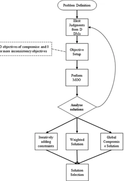
The main stages of the proposed approach are shown inFig. 1. The approach facilitates inconsistency reduction within the aggregation process via incorporating additional optimization objectives looking to find aggregated consensus solutions with minimal amounts of ordinal and or cardinal inconsistency.
The stages of our approach can be summarized as follows:
1. The number of elements of the problem is defined.
2. Judgements are elicited from each DM pertaining to their preferences between the elements of the problem. 3. The objectives for the MOO process are selected, consisting both of objectives of compromise to each DMs’ views as
well as optional additional inconsistency objectives.
4. The set of objectives are utilized within MOO to find the set of Aggregated Consensus Solutions.
5. Analysis of the set of Aggregated Consensus Solutions is performed to aid towards the selection of a single solution from the set of solutions. Such analysis may take one or more forms:
i. Analysis of the set of found Aggregated Consensus Solutions with respect to the levels of conflict between the DMs. The DMs can then iteratively add feasible constraints to gradually drill down to a sub-region of the objective space to help reach a final group consensus.
ii. Analysis can be performed utilizing weights of the importance of each DM to help identify a solution for which the compromise to each DMs’ views is proportional to their weights.
iii. Analysis utilizing information pertaining to the global levels of compromise in the group to help identify a solution which represents the least overall compromise to the group of DMs.
iv. Analysis of the Aggregated Consensus Solutions and their conflict may also aid identification of scenarios with unac-ceptable levels of conflict within the group (in the DMs’ eyes) in which amendment and update of the DMs’ judge-ments may be valuable.
3.1. Multi-objective optimization
In such an approach, due to the conflicting nature of the objectives, there will not be a single solution that optimizes all the objectives. Instead a range of trade-off non-dominated solutions will exist. A non-dominated solution is one that cannot
be declared inferior to any other solution. For these non-dominated solutions any improvement in one of the objectives will result in a decrease within one or more of the other objectives. The members of the set of non-dominated solutions are ter-med Pareto optimal solutions and together they map out the trade-off boundary edge –the Pareto front– of the problem.
3.2. Problem statement
Given a problem withnelements andDdecision makers who each define a completenbyn PCMof their judgments: PCM1;PCM2;. . .;PCMD
f g ð4Þ
From Eq.(1)we can see that the reciprocal judgments represent inferable information, therefore the minimum number of judgmentsðJÞneeded to construct a complete PCM ofnelements is:
J¼n nð 1Þ=2 ð5Þ
Thus, from a completed PCM, a Judgment SetOof cardinalityJcan be selected, containing enough information to recon-struct the whole of the PCM.Ocan be represented as the upper triangle of a PCM. Therefore our approach models anO rep-resentation of each DM’s PCMfO1;O2;. . .;OD}, each of which consists ofJjudgmentsfok1;ok2;. . .;okJg, fork = 1,. . .,D.
We seek the set of non-dominated Aggregated Consensus Solutions. Again we can represent each as a judgment set of cardinalityJ, denoted asA¼a1;a2;. . .;aJ. The set A represents the decision variables that can be obtained by minimizing a set of objectivesK.
The MOO problem can be formulated as:
Minimize½
K
ð6Þwhere
K
¼fE;BgThe set of objectivesKconsists of two subsets. The first subset E represents measures of compromise objectives
e
ið ÞA of cardinalityD, that each seek to minimize the measure of compromise wh respect to the correspondingOof a DM. This subset is defined as:E¼f
e
1ð Þ;Ae
2ð Þ;A . . .e
Dð ÞAg ð7ÞThe second subset B represents inconsistency objectivesbið ÞA of cardinalitym.
B¼fb1ð Þ;A . . .;bmð ÞAg ð8Þ
The approach additionally allows each DM to set constraints upon the amounts of compromise they are willing to tolerate in the pursuit of reaching a consensus. They can be employed to define an upper limit to the amount of a measure of com-promise that a DM’s judgments can undergo during optimization.
For example, given a constraint fromDMiofci upon their measure of compromise, the following constraint could be defined:
e
ið ÞA 6ci ð9ÞConstraints can additionally be set upon inconsistency objectives, this way defining bounds upon the amount of incon-sistency permitted within found aggregated consensus solutions. Thus a constraintfjupon an inconsistency objectivebjfrom objective subset B is defined as:
bjð ÞA 6fj ð10Þ
So, the constrained multi-objective optimization problem can be formulated as:
MinimizefE;Bg ð11Þ
subject to
e
ið ÞA 6cibjð ÞA 6fj
for i¼1;2;. . .;D and j¼1;2;. . .;m
Our approach then seeks to simultaneously optimize this set of objectives to find the trade-off front of the problem. A weights vector can then be derived from any of the aggregated consensus solutions found.
Evolutionary Computing (EC) techniques, such as Multi Objective Genetic Algorithms (MOGA)[6], can be used to solve the above problem and generate a set of non-dominated solutions. MOGA, such as those proposed in[10,22,21], seek to find a set of trade-off solutions, which are both as close to the true trade-off surface of the problem as possible and are as evenly spread along the trade-off front as possible. An application of a MOGA algorithm for solving the problem is discussed in Section4. Discussions on the definition and implementation of constraints within the approach are also presented in this section.
From the discovery of the trade-off front of the problem, with respect to the set of objectives, measures concerning the conflict between the DMs can be determined. For a group of DMs the approach can extract the measure of conflict between each pair of DMs, with respect to the chosen measure of compromise, and create a ranking of the set of pairs. This can be calculated from the inter-distance measure of compromise between each pair within the objective space. This allows iden-tification of DMs with closely matching views, as well as DMs for which there is a high level of conflict, helping to give a deeper understating of the nature of the group of DM’s views. The approach can further calculate an average of these pairings to derive a measure of agreement for each DM. These values when ranked can then highlight the ‘‘most agreeable’’ DM, who is most representative of the whole group and also the ‘‘most disagreeable’’ DM, whose views are the most outlying.
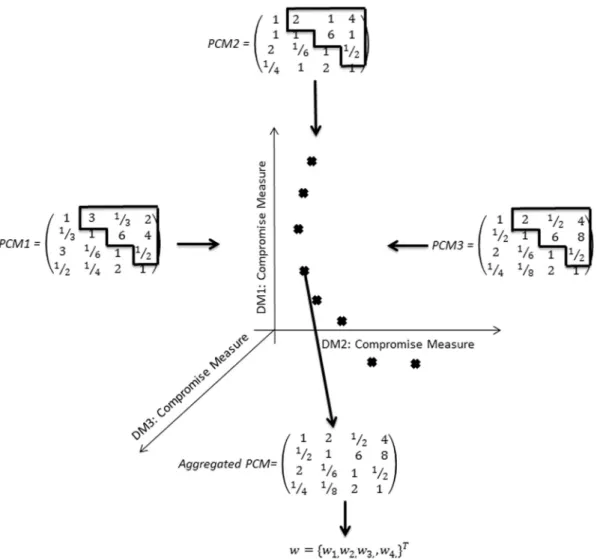
Fig. 2illustrates an objective space found using the approach for a 4 element, 3 DM problem. Each axis represents a com-promise measure objective denoting comcom-promise for each DM. Additional inconsistency objectives could also have been employed increasing the number of dimensions of the objective space. A set of trade-off aggregated consensus solutions (in this case 8) have been found and their measures with respect to the amount of compromise to each DM are shown through their position within the objective space. From an aggregated consensus solution a final ranking weights vector of the 4 elements under consideration can then be derived.
Next the measures of compromise that can be selected as objectives for the approach are outlined, followed by the mea-sures of inconsistency that may be utilized as additional objectives within the approach.
3.3. Measures of compromise
Given a DM judgment set (O) represented as a set of judgmentsfo1;o2;. . .;oJgof cardinalityJ. The amount of change betweenO and a secondAggregated judgment set (A) of judgmentsa1;a2;. . .;aJ can be calculated using a variety of
measures. Each measure can be employed by a DM as an objective to measure the compromise between their judgments and an aggregated consensus solution.
3.3.1. Number of Judgment Violations (NJV)
NJV is a measure of the number of the original set of PC judgments that have changed, without consideration of the amount of change of each judgment; wheredevaluates to 0 or 1 for each Boolean evaluation.
NJV¼X
J
j¼1
doj!¼aj ð12Þ
3.3.2. Total Judgment Deviation (TJD)
TJD is a measure of the total amount of change between the original judgments and an altered judgment set. It takes into consideration the amount of preference change between each judgment comparison.
TJD¼X J j¼1 ojaj ð13Þ
A modified version of the TJD measure is the Squared Total Judgment Deviation (STJD). Here the deviations between the corresponding judgments in both sets are squared; consequently altered judgments with a large alteration in strength will have a greater impact upon the measure’s total.
STJD¼X J j¼1 ojaj 2 ð14Þ The TJD can be extended further by taking the square root of the STJD value resulting in the Euclidian Total Judgment Deviation (ETJD), representing a measure of the Euclidian Distance between the two judgments sets.
ETJD¼ ffiffiffiffiffiffiffiffiffiffiffiffiffiffiffiffiffiffiffiffiffiffiffiffiffiffiffiffiffiffiffiffiffi XJ j¼1 ojaj 2 r ð15Þ
3.3.3. Number of Judgment Reversals (NJR)
NJR is a measure of the number of judgments from the original set that have been inverted in an altered judgment set. For example, given an original judgment between elementsxandywherexy: if in an altered judgment set it is the case that x ythen a judgment reversal has occurred. This measure of compromise also considers half reversals. Half reversals are defined as occurring when a judgment of equal preference is altered to be a judgment of not equal preference or a judgment not of equal preference is altered to be a judgment of equal preference. Using the 1–9 scale we can specify equal preference, greater than equal preference and less then equal preference, as 1, greater than 1 and less than 1 respectively.
NJR¼X J j¼1 Rj ð16Þ where Rj 1:oi>1and ai>1 1:oi<1and ai<1 0:5:oi¼1and ai–1 0:5:oi–1and ai¼1 0:otherwise 8 > > > > > > < > > > > > > :
3.4. Inconsistency reduction objectives
As well as the measures of compromise objectives, additional objectives of both ordinal and/or cardinal inconsistency measures can be incorporated into the MOO approach. Together they make up the objective subset B of the approach. This will result in seekingAggregated Consensus Solutionswith low levels of inconsistency. Ordinal inconsistency can be con-sidered through employing the number of 3-way cycles (L) as an inconsistency reduction objective[19], looking to minimize the number of cycles within Aggregated Consensus Solutions. Cardinal inconsistency can be considered through utilizing the Consistency Ratio (CR)[27] as an inconsistency reduction objective. Constraints can also be set upon any inconsistency objectives from objective subset B. For example, to adhere to Saaty’s recommended CR < 0.1 threshold level of acceptability of inconsistency[27], an upper limit constraint of 0.1 can be set upon a CR inconsistency reduction objective.
3.5. Selecting a single non-dominated solution
For real-world decision making problems as well as seeking to find a set of trade-off solutions for problems with multiple conflicting objectives, additional consideration needs to be given to ultimately help a single solution to be selected[25]. Such support towards aiding the selection of a single solution can be divided into 3 categories – based on when DM preferences are incorporated into the search process to find trade-off solutions.
1. A priori: Here DM preferences are incorporated before the search for trade-off solutions. Such approaches generally attach weights to the objectives before the search process, see[7]. Such strategies assume that such preferences are known and clear from the start of the problem, which is rarely the case and hence can result in having to re-run the process if these preferences are altered. Moreover attempting to extract direct preference information first may be so consuming and complex that it is counterproductive to real world decisions[3]. Our approach incorporates some less direct a priori preference information relating to the number of solutions sought. Our approach utilizes a MOGA with an external archive that controls the maximum number of solutions that are returned from the MOO search process. Thus we incorporate into the search process some DM preferences, to seek to present a suitable number of trade-off solutions to the DMs. The implementation of a MOGA and an archive within our approach is discussed in Section4.1. 2. Interactive: Alternatively DM preferences can be incorporated progressively during the searching via interactive feedback such as in[24], in which DM preferences are incorporated by presenting pairs of non-dominated solutions for discrimination between, and in[12], where a utility function of DM preferences is utilized to help drive the search process into preferred areas of the trade-off front. Our approach utilizes constraints added iteratively within multiple searches to reduce the size of the objective space towards feasible areas of interest expressing each DM’s tolerance levels represented as constraints. This helps facilitate selection towards a single compromise solution through iter-atively reducing the objective space size. Utilizing constraints without our approach is outlined in Section3.2. 3. Posteriori: Finally DM preferences may also be incorporated after the search. Our approach implements multiple
ways to aid DMs in the selection of a single solution after our MOO search process, either through utilizing informa-tion pertaining to the global measures of compromise within the group or through employing informainforma-tion relating to the weights of importance of each DM. The identification of such solutions can then aid the DMs in the selection of a final solution.
3.5.1. Utilizing global measures of compromise to select a single solution
Through the calculation of information pertaining to the global levels of compromise within the group a single solution can be identified that represents the least amount of overall compromise for the group of DMs. For each aggregated consen-sus solution found, a global measure of the total compromise of the type used by the DMs as objectives can be calculated. This represents the sum of the compromise measure value for each DM for the chosen measure of compromise. For example, the global total number of judgment reversalsTNJRforDDMs can be calculated via:
TNJR¼X D i¼1 XJ j¼1 Rj ð17Þ
Global measures of compromise for the other measures of compromise SJD and NJV can be calculated in a similar way. From this, a ranking of the set of aggregated consensus solutions can be made with respect to their global measure of com-promise, from which the solution with the lowest global measure of compromise can be selected and a weights vector derived – aGlobal Consensus weights vector.
Generally there will be a sub-set of aggregated consensus solutions that share the lowest total measure of compromise value –Global Aggregated Solutions. In this case the approach calculates a single weights vector as the average (utilizing the geometric mean) of the weight vectors derived from this sub-set of aggregated consensus solutions. In this way a Global Consensus weights vector is found that represents the average of the sub-set of solutions within the region of the trade-off front with least overall compromise. Utilizing the geometric means to perform the averaging will lessen the effects of outliers.
For the examples presented later the Geometric Mean PM[9](equivalent to the Logarithmic Least Squares (LLS) PM[9]) is utilized to derive weights vectors from aggregated consensus solutions, however any PM can be utilized. Additionally, as the approach actively seeks aggregated consensus solutions with low inconsistency, the choice of PM becomes less significant.
3.5.2. Utilizing DM weights of importance to find a weighted single solution
Alternatively a single solution can be sought via incorporation of an additional set of weights of importance for each DM. These weights are incorporated after the search process to identify the solution with levels of compromise for each DM pro-portional to their weight of importance. Consequently through the altering of the set of DM weights, sensitivity analysis can examine how changes to the DM weights of importance affect the selected weighted solution. As the front of aggregated con-sensus solutions has been found such sensitivity analysis can be performed without the need to re-run the MOO search pro-cess (which would be required for weights incorporated into the objectives before the search propro-cess). The approach takes the set of weights of importance of each DM and utilizes them to identify a solution along the front of aggregated consensus
solutions proportional to the weights of each DM. This way the higher weighted a DM is, the smaller amount of compromise their judgments will undergo to reach a consensus.
In the next section the approach and its benefits are explored through illustrative examples.
4. Illustrative examples
In this section step-by-step examples of our approach are presented following an overview of its implementation. Example 1 explores the aggregation process, then analysis of the set of solutions found is performed through:
1. Analysis pertaining to the levels of conflict between the DMs followed by the adding of feasible constraints to explore the solutions space.
2. The selection of a single solution utilizing global measures of compromise knowledge. 3. The selection of a single solution utilizing DMs’ weights of importance.
Example 2 looks at how inconsistency reduction can be incorporated during the aggregation process, then analysis of the set of solutions found is utilized to help in selection of a single solution.
4.1. Approach implementation
Our approach is implemented utilizing the MOCell MOGA[21], in which the population of individuals is arranged as a two-dimensional grid and an external archive is used to store the set of non-dominated solutions found so far. An archive gives additional control over the final number of solutions found. Restrictive mating is utilized, in which individuals are selected to mate only with those individuals in close proximity to them in the grid, to ensure diversity is preserved for longer within the population. Additionally the mechanism of feedback is used to add a given number of the best solutions found so far back into the population at the start of each generation to help stimulate convergence towards the problem’s Pareto front. Both soft and hard constraints are employed for the implementation of constraints within the approach. Soft constraints have been implemented into the approach utilizing Constrained Pareto Dominance[10]as defined as the constraint handling procedure within the Non-dominated Sorting Genetic Algorithm-II (NSGAII)[10]. Constrained Pareto Dominance constraints are taken into account during the selection phase of the MOGA operation by considering the feasibility of solutions with respect to any constraints and favouring a feasible solution over an infeasible one. The effect of this soft constraint is to push the population towards feasible regions of the objective space. An additional hard constraint is employed to only allow fea-sible solutions to be added to the archive.
The examples that follow were executed employing the following parameter settings: population size of 100 (1010 grid); maximum evaluations count of 25,000; archive size dynamically defined based upon the number of DMs and objec-tives within the problem with a feedback value of one-quarter the size of the archive. Selection is performed via binary tour-nament (see[13]for more details) with single point crossover (with crossover probability 0.9) and bit flip mutation (with probability 0.01) employed (see[15]for discussions of crossover and mutation).
4.2. Example 1
4.2.1. Two decision makers (1a)
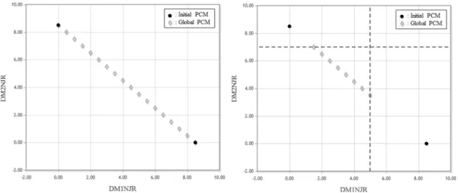
Given a set of 6 elements, PCM judgments from 2 DMs as shown inTable 1, and NJR chosen as the measure of compromise for each DM, the objective space of the set of non-dominated aggregated consensus solutions found is shown inFig. 3: Left. Having found the trade-off front of solutions, analysis of these non-dominated solutions can then be performed.
We can observe the trade-off front from one edge representing no compromise to one DM’s judgments and the largest compromise in the other DMs judgments, and vice versa at the other edge of the front. Between these edges a range of com-promise solutions map out the trade-off front. Here we observe the amount of conflict between the pair: a minimum of 8.5 total NJR is needed to reach a consensus. We can see that each solution along the front represents a global aggregated
Table 1
Example 1a: DM1 and DM2 PCMs.
DM1 DM2 1 2 3 4 5 6 1 2 3 4 5 6 1 1 1/5 1/2 7 1/8 1/5 1 7 1/3 5 8 1/4 2 5 1 3 8 8 1/9 1/7 1 1/7 1/5 1 1/9 3 2 1/3 1 1/2 1/9 6 3 7 1 2 5 5 4 1/7 1/8 2 1 2 4 1/5 5 1/2 1 1/2 1/4 5 8 1/8 9 1/2 1 1/9 1/8 1 1/5 2 1 1/4 6 5 9 1/6 1/4 9 1 4 9 1/5 4 4 1
solution as each shares the lowest total NJR value. From this set of global aggregated solutions we can derive a single global consensus weights vector, from the average of the weights vector of each global aggregated solution, shown inTable 2.
Additionally we can utalize constraints to allow the DMs to explore and focus in on sub-regions of the objective space. From the initial objective space obtained, the DMs can set feasible constraints now that the amount of conflict between the pair has been determined. For example, DM1 could set an upper tolerance constraint of an NJR value of 5, and DM2 could set an upper tolerance constraint value of 7 NJR. The new objective space calculated with the added constraints is shown in Fig. 3: Right. From this we see the number of global aggregated solutions has been reduced to 8, from which a global con-sensus weights vector can be derived and is shown inTable 3. As DM1 defined a stricter judgment reversals constraint the derived global consensus weights vector will more closely reflect their judgments than the previously calculated global con-sensus weights vector.
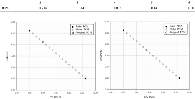
Furthermore we can analyze the set of Aggregated Consensus Solutions found incorporating knowledge pertaining to the weights of importance of each DM. Given further DM weights of importance, i.e. 0.75 for DM1 and 0.25 for DM2, we can identify a weighted solution that most meets their weights proportions through calculating the nearest aggregated consen-sus solution on the front as highlighted inFig. 4: Left. Form this selected weighted aggregated consensus solution the derived weights vector is shown inTable 4.
As the trade-off front of the problem has been determined, sensitivity analysis regarding altering the DM weights of importance can be performed without having to re-run the approach. For example the effects of altering the DM weights to 0.6 for DM1 and 0.4 for DM2, are shown inFig. 4: Right with the weights vector derived from the selected weighted aggre-gated consensus solution shown inTable 5.
4.2.2. Four decision makers (1b)
When there are only two DMs, the trade-off front in the two-dimensional space will be a one-dimensional plane in which the knowledge extraction is rudimentary – we saw inFig. 3that all solutions found shared the same global NJR value of 8.5. The knowledge extraction becomes more valuable when more than two DMs are involved. Therefore, the example is extended to 4 DMs, of which the PCM judgments for DM3 and DM4 are shown inTable 6. Again NJR was chosen as the mea-sure of compromise for each DM.
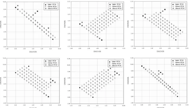
Fig. 5shows the found four-dimensional trade-off surface from a set of two-dimension views for each pairing of DMs. From these views of the trade-off front, the surface edges with respect to each pairing are visible.
We observe the linear trade-off between each pair of DMs and calculate the level of conflict between each pair via the inter-distance in the objective space between the pair. By extracting the value of this measure for each pair of DMs we can gauge and rank the amount of conflict between each pairing in the group. The values for each of the 6 pairings in our example are shown inTable 7. From this we can see that the mostagreeing pair are DM2 and DM4 and that the most
Fig. 3.Left: Example 1a objective space. Right: Example 1a constrained objective space.
Table 2
Example 1a: Global consensus weights vector derived from the set of global aggregated solutions.
1 2 3 4 5 6
disagreeingpair are DM3 and DM4. By additionally calculating the averages for each pairing a DM is involved in, shown in Table 8, we can observe the overall ‘‘most agreeable’’ DM is DM2 and the ‘‘most disagreeable’’ is DM3.
Additionally fromFig. 5, we observe from the set of all aggregated consensus solutions found that there is a sub-set of solutions which share the lowest global NJR value (19) from which a Global Consensus weights vector can be derived, shown inTable 9.
4.3. Example 2: incorporating inconsistency reduction
Example 1 illustrated how aggregated consensus solutions are determined through looking to minimize the compromise for each DM. Example 2 illustrates how the approach additionally incorporates inconsistency reduction into the consensus
Table 3
Example 1a: Global consensus weights vector derived from the set of global aggregated solutions with constraints.
1 2 3 4 5 6
0.099 0.214 0.144 0.092 0.143 0.309
Fig. 4.Left: Example 1a DM weighted selection. Right: Example 1a altered DM weighted selection.
Table 4
Example 1a: weights vector derived from set of DM weights.
1 2 3 4 5 6
0.179 0.191 0.089 0.170 0.081 0.289
Table 5
Example 1a: weights vector derived from altered set of DM weights.
1 2 3 4 5 6 0.116 0.331 0.273 0.085 0.046 0.149 Table 6 Example 1b: DM3 and DM4 PCMs. DM3 DM4 1 2 3 4 5 6 1 2 3 4 5 6 1 1 3 8 1/7 1/5 1/5 1 1/7 1 5 4 1/4 2 1/3 1 3 8 8 1/9 7 1 1/7 1/5 1 1 3 1/8 1/3 1 2 1/9 6 1 7 1 2 5 5 4 7 1/8 1/2 1 2 1/4 1/5 5 1/2 1 1/2 4 5 5 1/8 9 1/2 1 1/4 1/4 1 1/5 2 1 1/4 6 5 9 1/6 4 4 1 4 1 1/2 1/4 4 1
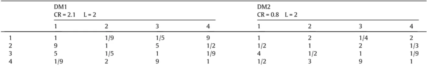
process to reduce its adverse effects. For a 4 element set, PCM judgments from 2 DMs are shown inTable 10along with initial measures of cardinal and ordinal inconsistency CR and L. We seek the trade-off front of aggregated consensus solutions with STJD chosen as the measure of compromise for each DM and additionally look to simultaneously minimize the inconsistency of found aggregated consensus solutions.
To help find more consistent aggregated consensus solutions, which reduce the effects of the DM’s inconsistency, we can incorporate inconsistency reduction with an additional third objective of CR. We can also define a constraint upon this
Fig. 5.Example 1b: Views of objective space for each pairing of DMs.
Table 7
Example 1b: Agreement values between each pair of DMs.
DM pair Min TNJR 1&2 8.5 1&3 5 1&4 7.5 2&3 7.5 2&4 3 3&4 9.5 Table 8
Example 1b: Average agreement values of each DM.
DM Avg. TNJR 1 7.00 2 6.33 3 7.33 4 6.67 Table 9
Example 1b: Global consensus weights vector derived from set of global aggregated solutions.
1 2 3 4 5 6
objective of an upper limit of 0.1.Fig. 6: Left shows the three-dimensional objective space from the view of STJD of each DM. From this we see there are three global aggregated solutions, all of which will be below the 0.1 CR threshold, from which a calculated global consensus weights vector is shown inTable 11.
The approach allows both cardinal and/or ordinal inconsistency reduction to be incorporated into the aggregation process to suit the DMs needs and preferences. We can instead employ a third objective of L and additionally set a constraint upon it to limit the number of 3-way cycles in aggregated consensus solutions found.Fig. 6: Right shows the aggregated solutions found with STJD utilized as the measure of compromise for each DM and this time a third objective of L employed with an additional constraint of L = 0. We see that a number of aggregated consensus solutions have been found all of which will contain no cycles. Having found the trade-off front of solutions, analysis of these non-dominated solutions can be performed. For example, we can derive a global consensus weights vector, shown inTable 12, from the sub-set of the global aggregated solutions sharing the lowest total STJD.
Table 10 Example 2: DM1 and DM2 PCMs. DM1 DM2 CR = 2.1 L = 2 CR = 0.8 L = 2 1 2 3 4 1 2 3 4 1 1 1/9 1/5 9 1 2 1/4 2 2 9 1 5 1/2 1/2 1 2 1/3 3 5 1/5 1 1/9 4 1/2 1 1/9 4 1/9 2 9 1 1/2 3 9 1
Fig. 6.Left: Example 2: STJD measure of compromise with CR as an additional 3rd objective with CR < 0.1 constraint. Right: Example 2: STJD measure of compromise with L as an additional 3rd objective with L = 0 constraint.
Table 11
Example 2: Derived global consensus weights vector from STJD measure of compromise and CR and CR < 0.1 constraint.
1 2 3 4
0.117 0.373 0.086 0.423
Table 12
Example 2: Derived global consensus weights vector from STJD measure of compromise and L and L = 0 constraint.
1 2 3 4
4.4. Summary of examples and approach
We have demonstrated our approach to the problem of aggregation of PC judgments of a group of DMs for differing num-bers of DMs, measures of compromise and inconsistency measures. To summarize, the aggregation is performed with respect to looking to explicitly optimize the amount of compromise for each DM. The approach gives flexibility as to how compro-mise is to be measured, to suit the needs of the DMs and the decision problem. The approach allows constraints to be defined to act as tolerance levels of compromise for each DM. Adoption of a MOO methodology allows the discovery of the trade-off front of the problem for the objectives set to be found, enabling understanding of both the nature of the problem and the conflict between the different DMs. This additionally allows the setting of more feasible constraints by the DMs. Moreover, the approach incorporates inconsistency reduction during the aggregation process. Either ordinal or cardinal inconsistency, or both, can be utilized in the approach and constraints upon levels of inconsistency can also be set. Finally, when utilizing a set of DM weights of importance, sensitivity analysis can swiftly be performed upon weighted solu-tions found without re-running the approach.
5. Case study: analytic hierarchy process
We now present a step-by-step case study to illustrate the use of our approach within an MCDM Analytic Hierarchy Process (AHP) decision problem framework. Our approach has been applied to the aggregation of PC judgments of a group of DMs whilst also looking to reduce inconsistency during the aggregation process. Firstly, a brief overview of AHP is given, and then an AHP decision problem is undertaken using our approach to derive a final ranking of the alternatives pertaining to the problem. Discussions and comparisons of our aggregation approach compared to the GMM aggregation approach are dis-cussed during the stages of the decision problem.
5.1. Analytic Hierarchy Process (AHP)
AHP, developed by Saaty[29], makes extensive use of PCs utilized within a hierarchical framework defining the decision goal, its alternatives and the set of criteria for which the alternatives are to be compared by. AHP can be utilized for both single and group decision making problems. The AHP procedure can be broken down into four broad stages. Firstly, the Problem’s Goal, Criteria, and Alternatives are defined and a hierarchy constructed. Next, DM preferences are elicited from which PCMs are constructed. The elements on a single layer are compared with respect to the dependencies they share with the level above them in the hierarchy.
Once all judgments have been elicited, judgments are aggregated to arrive at a ranking for each element at that layer with respect to each element in the layer above, creating a weights vector ranking of the elements from each PCM. Within a group setting various approaches exist regarding how synthesis between the PCMs of multiple DMs are incorporated into the derivation of a group weights vector as discussed in Section2. Finally, synthesis of the weight vectors at each level of the hierarchy is performed to arrive at a final ranking of the decision alternatives. For a full overview and discussion of AHP see[29].
5.2. Case study
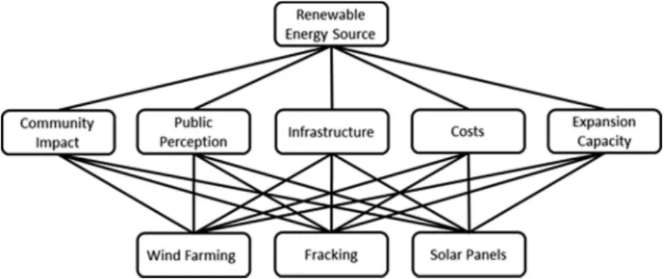
The case study explores a group of 3 DMs presiding over the choice of a new renewable energy source initiative within the community. The first stage of AHP pertains to the formulation of the decision and its elements.
5.2.1. Formulation of decision problem
When AHP is utilized for group decision making the formulation of the decision’s elements may be defined by a single overseeing DM or via a more interactive approach between the DMs involved[29]. In our case study we have an overseeing DM, and 5 criteria and 3 alternatives have been identified from which the 3 DMs preferences will be elicited. The 3 alterna-tives are:
A1: Wind Farming (WF) A2: Fracking (F) A3: Solar Panels (SP)
The 5 criteria to which the alternatives are to be compared with respect to are:
C1: Community Impact: The short-term and long-term impacts upon the community and land from the energy sources (CI)
C2: Public Perception: Perceived support and perceptions of the local community towards each type of energy source (PP) C3: Infrastructure: The set-up and deployment factors of each energy source along with accompanying legislation
C4: Costs: Considerations of the costs of both initial setup and maintenance costs associated with each energy source (Co) C5: Expansion Capacity: The ease of future development and expansion capabilities of each energy source (EC).
With the elements of our decision defined we can construct the AHP hierarchy, as shown inFig. 7, and start eliciting judg-ments from the DMs. For the aggregation at each elicitation stage within our approach the measure of compromise utilized will be NJV for each DM and an additional objective of CR will be employed with an added upper constraint threshold of 0.1. At each aggregation stage a Global Consensus weights vector is sought by taking the average from the sub-set of global aggregated solutions sharing the lowest total measure of compromise (in this caseTotal NJV).
5.2.2. Judgment elicitation and analysis
Judgments may be elicited in any order but here we first analyze the elicitation of the preference of criteria from the DMs, then analyze the elicitation of DMs’ preferences between the alternatives with respect to each criterion.
5.2.2.1. Elicitation, aggregation and analysis of criteria priorities.To determine the importance of each criterion, we elicit
judg-ments from the DMs with respect to the decision goal, as shown inFig. 8, and then derive the criteria weights vector. The three PCMs of preferences from the DMs for the importance of each criterion are shown inTable 13along with incon-sistency values for each DM.
As well as utilizing our MOO approach we can calculate a criteria weights vector using the GMM for comparison against our approach. For the GMM, the PCM created as the aggregation of this information is shown inTable 14. We can see that the
Fig. 7.Hierarchy representation of the decision problem.
Fig. 8.Criteria with respect to the problem.
Table 13
AHP PCM relating to criteria preferences of the three DMs.
DM1 DM2 DM3 CR = 0.54 L = 2 CR = 0.5 L = 3 CR = 0.7 L = 3 CI PP I Co EC CI PP I Co EC CI PP I Co EC CI 1 1/4 1/7 1 1/4 1 1/5 2 1 5 1 1/8 1/7 1/9 5 PP 4 1 1/2 1/2 6 5 1 1 3 1/3 8 1 1/4 1/2 1/3 I 7 2 1 1/2 3 1/2 1 1 1/2 1/2 7 4 1 1/2 6 Co 1 2 2 1 1/6 1 1/3 2 1 4 9 2 2 1 1/2 EC 4 1/6 1/3 6 1 1/5 3 2 1/4 1 1/5 3 1/6 2 1
level of cardinal inconsistency is above the 0.1 threshold level and consequently any weights vector derived from it will lack accuracy. However, our MOO approach with its constrained CR objective will only derive aggregated PCMs with CR values below the 0.1 threshold thus facilitating more accurate weights vector estimates to be derived.
The weights vectors relating to the criteria weights derived from the two aggregation approaches are shown inTable 15, with the most important criterion for each approach shown in bold. We see that the most important criterion calculated from the GMM is Infrastructure, whereas the most important criterion calculated from our MOO approach is Costs. As we have seen the variation in the weights can be attributed to our MOO approach being able to consider the additional infor-mation regarding inconsistency reduction.
5.2.2.2. Eliciting, aggregation and analysis of alternatives priorities with respect to each criterion. For the 3 alternatives we also
elicit judgments from our DMs of their preferences between the alternatives for each criterion. For example we can first determine the preferences of the DMs between the alternatives with respect to the Expansion Capacity criterion, shown in Fig. 9. The weights vectors derived from the DMs’ preferences of the alternatives with respect to the Expansion Capacity criterion, using our MMO approach and the GMM, are shown inTable 16.
The aggregated PCM calculated during the GMM process has a CR value greater than 0.3, again above the threshold of acceptable inconsistency. Conversely any aggregated PCM calculated during our MOO approach, with the added constraint upon the CR objective, will find PCMs below our 0.1 threshold. We see the effects of this inTable 16with our MOO approach producing a differing ranking to the GMM approach regarding the 2nd and 3rd most preferred alternatives.
In the same manner, we can elicit judgments from the DMs of the alternatives with respect to the other 4 criteria, and then derive aggregated weights vectors using our MOO approach, as shown inTable 17, with the most preferred alternative for each criterion shown in bold.
Table 14
Aggregated PCM from GMM of the criteria preferences. CR = 0.18 L = 3 CI PP I Co EC CI 1 0.18 0.34 0.48 1.84 PP 5.43 1 0.5 0.91 0.87 I 2.9 2 1 0.5 2.08 Co 2.08 1.1 2 1 0.69 EC 0.54 1.14 0.48 1.44 1 Table 15
AHP aggregated criteria weights from MOO and GMM.
Community impact Public perception Infrastructure Costs Expansion Capacity
GMM 0.107 0.221 0.272 0.239 0.160
MOO 0.121 0.124 0.241 0.355 0.159
Fig. 9.Alternatives compared with respect to Expansion Capacity criterion.
Table 16
AHP aggregated alternative weights vectors with respect to Criterion 5 for MOO and GMM.
C5 Wind farming Fracking Solar panels
GMM 0.229 0.408 0.363
5.2.3. Synthesis to a final ranking
With all the judgments elicited and weights vectors derived, the next stage is the synthesis of these weights vectors into a final ranking of the alternatives. The resulting final ranking of the alternatives produced via our MOO approach and via the GMM approach are presented inTable 18, with the most preferred alternative for each approach shown in bold. From these rankings from the 2 approaches we see that a differing final ranking has been determined from our MOO approach compared to the GMM approach. The highest ranking alternative from the GMM is Solar Panels; whereas for our MOO approach Wind Farming is the highest ranking alternative. Considering this differing final ranking, we have seen from the intermediate stages of the aggregation process that our MOO method considers more information and explicitly incorporates inconsis-tency reduction, thus a richer ranking has been obtained.
5.2.4. Case study conclusions
We have observed through the Case Study that as our MOO method facilitates explicit incorporation of inconsistency reduction during aggregation a richer ranking can be obtained. Moreover our MOO methodology facilitates an indicator-based approach to the aggregation process, in that DMs can decide how compromise during aggregation will be measured through choice over the measure of compromise to use. In our example NJR was utilized, however TJD for example could have been utilized. Likewise how inconsistency is to be measured (if at all) can again be chosen: in the case study we used the CR objective, however L could also or instead have be utilized.
There are also additional analysis benefits that our approach facilitates that we can use. Knowledge measures could be utilized at each aggregation stage to glean knowledge of the conflicts between the DMs. Constraints on measures of compro-mise could be employed at each aggregation stage to help drill down towards the selection of a single solution from which to derive a weights vector from. Moreover weights of importance of each DM could be incorporated at each aggregation stage.
6. Conclusions
We have presented an approach to the aggregation of PC judgments of a group of DM’s utilizing MOO. The aggregation is performed aiming to explicitly optimize the amount of compromise for each DM. The approach gives flexibility as to how compromise is to be measured. Constraints can be defined upon a measure of compromise objective to act as tolerance levels of compromise for each DM.
The adoption of a MOO methodology allows the discovery of the trade-off front of the problem to be found allowing understanding of the nature of the problem and the conflict between the DMs to be revealed. This can additionally facilitate the setting of more feasible tolerance constraints by the DMs.
The approach additionally incorporates inconsistency reduction during the aggregation process. Reduction of ordinal or cardinal inconsistency or both can be incorporated into the process. Constraints can also be set upon inconsistency objectives to set threshold levels of inconsistency acceptable within aggregated solutions found.
The approach can be utilized to select a single solution, either through utilizing the global measure of compromise infor-mation or through incorporating DM weights of importance. When utilizing a set of DM weights of importance sensitivity analysis can be performed upon altered weights of importance without re-running the approach. Finally, the approach can be applied within MCDM frameworks such as AHP.
Further work will investigate decisions in which the number of DMs is large and explore utilizing total measures of com-promise information to aid the clustering of DMs based on the similarly of their judgments. Further knowledge measures pertaining to identifying conflict within a group of DMs will also be investigated.
Table 17
AHP aggregated weights vectors for alternatives respect each criterion.
Wind farming Fracking Solar panels
Community impact 0.122 0.320 0.558 Public perception 0.165 0.225 0.610 Infrastructure 0.661 0.131 0.208 Costs 0.493 0.196 0.311 Expansion Capacity 0.286 0.571 0.143 Table 18
AHP final alternatives rankings for MOO and GMM approaches.
GMM MOO
Wind farming 0.367 0.415
Fracking 0.256 0.259
Acknowledgment
Abel acknowledges the support of the Engineering and Physical Science Research Council (EPSRC) via their doctoral train-ing grant.
References
[1] E. Abel, L. Mikhailov, J. Keane, Reducing inconsistency in pairwise comparisons using multi-objective evolutionary computing, in: 2013 IEEE International Conference on Systems, Man, and Cybernetics (SMC), 2013, pp. 80–85.
[2]J. Aczél, T.L. Saaty, Procedures for synthesizing ratio judgements, J. Math. Psychol. 27 (1) (1983) 93–102.
[3]J. Branke, S. Greco, R. Słowi’nski, P. Zielniewicz, Interactive evolutionary multiobjective optimization using robust ordinal regression, in: Evol. Multi-Crit. Optim., Springer, 2009, pp. 554–568.
[4]J. P Brans, B. Mareschal, P. Vincke, PROMETHEE: a new family of outranking methods in multicriteria analysis, Oper. Res. 84 (1984) 477–490. [5]E.U. Choo, W.C. Wedley, A common framework for deriving preference values from pairwise comparison matrices, Comput. Oper. Res. 31 (6) (2004)
893–908.
[6]C. Coello Coello, Evolutionary multiobjective optimization a historical view of the field, IEEE Comput. Intell. Mag. 1 (1) (2006) 28–36. [7]C. Coello, G. Lamont, D. Van Veldhuizen, Evolutionary Algorithms for Solving Multi-objective Problems, Springer, 2007.
[8]J. Costa, A genetic algorithm to obtain consistency in analytic hierarchy process, Brazilian J. Oper. Prod. Manage. 8 (1) (2011) 55–64. [9]G.B. Crawford, The geometric mean procedure for estimating the scale of a judgement matrix, Math. Modell. 9 (3–5) (1987) 327–334. [10] K. Deb, A. Partap, T. Meyarivan, A fast and elitist multiobjective genetic algorithm, NSGA-II, IEEE Trans. Evol. Comput. 6 (2) (2002) 182–197. [11]E. Forman, K. Peniwati, Aggregating individual judgments and priorities with the analytic hierarchy process, Eur. J. Oper. Res. 108 (1998) 165–169. [12]J.W. Fowler et al, Interactive evolutionary multi-objective optimization for quasi-concave preference functions, Eur. J. Oper. Res. 206 (2) (2010) 417–
425.
[13]D.E. Goldberg, K. Deb, A comparative analysis of selection schemes using in genetic algorithms, in: Foundations of Genetic Algorithms, Morgan Kaufman, 1991, pp. 69–93.
[14]P. Harker, L. Vargas, The theory of ratio scale estimation: Saaty’s analytic hierarchy process, Manage. Sci. 33 (11) (1987) 1383–1403. [15]R. Haupt, S. Haupt, Practical Genetic Algorithms, John Wiley & Sons Inc., 2004.
[16] C.L. Hwang, K.P. Yoon, Multiple attribute decision making, Methods and applications, A state-of-the-art survey, 1981.
[17]A. Ishizaka, D. Balkenborg, T. Kaplan, Influence of aggregation and measurement scale on ranking a compromise alternative in AHP, J. Oper. Res. Soc. 62 (2010) 1–11.
[18]W. Koczkodaj, S. Szarek, On distance-based inconsistency reduction algorithms for pairwise comparisons, Logic J. IGPL 18 (6) (2010) 859–869. [19]M. Kwiesielewicz, E.V. Uden, Inconsistent and contradictory judgements in pairwise comparison method in the AHP, Comput. Oper. Res. 31 (2004)
713–719.
[20] F.A. Lootsma, Conflict resolution via pairwise comparison of concessions, Eur. J. Oper. Res. 40 (1) (1989) 109–116.
[21]A.J. Nebro, J.J. Durillo, F. Luna, B. Dorronsoro, E. Alba, A cellular genetic algorithm for multiobjective optimization, NICSO (2006) 25–36. [22]A.J. Nebro et al, AbYSS. Adapting scatter search to multiobjective optimization, IEEE Trans. Evol. Comput. 12 (4) (2008) 439–457. [23] S. Opricovic, Multicriteria Optimization of Civil Engineering Systems, Faculty of Civil Engineering, Belgrade, 1998.
[24]S.P. Phelps, M. Koksalan, An interactive evolutionary metaheuristic for multiobjective combinatorial optimization, Manage. Sci. 12 (2003) 1726–1738. [25] R.C. Purshouse, K. Deb, M.M. Mansor, S. Mostaghim, R. Wang, A Review of Hybrid Evolutionary Multiple Criteria Decision Making Methods, COIN
Report, 2014.
[26]R. Ramanathan, L.S. Ganesh, Group preference aggregation methods employed in AHP: an evaluation and an intrinsic process for deriving members’ weightages, Eur. J. Oper. Res. 79 (1994) 249–265.
[27]T.L. Saaty, A scaling method for priorities in hierarchical structures, J. Math. Psychol. 15 (3) (1977) 234–281.
[28]T.L. Saaty, Group decision making and the AHP, in: The Analytic Hierarchy Process, Applications and Studies, Springer, Berlin, 1989, pp. 59–67. [29]T.L. Saaty, The Analytic Hierarchy Process, Planning, Piority Setting, Resource Allocation, McGraw-Hill, New York, 1980.
[30] T.L. Saaty, L.G. Vargas, Decision Making with the Analytic Network Process, Springer, New York, 2008.
[31]S. Siraj, L. Mikhailov, J. Keane, A heuristic method to rectify intransitive judgments in pairwise comparison matrices, Eur. J. Oper. Res. 216 (2012) 420– 428.
[32]L. Thurstone, A law of comparative judgment, Psychol. Rev. 34 (4) (1927) 266–270.