©2016 The Authors Journal of the Royal Statistical Society: Series A (Statistics in Society) Published by John Wiley & Sons Ltd on behalf of the Royal Statistical Society.
This is an open access article under the terms of the Creative Commons Attribution-NonCommercial-NoDerivs License, which permits use and distribution in any medium, provided the original work is properly cited, the use is non-commercial and no modifications or adaptations are made.
0964–1998/16/180000
A space–time multivariate Bayesian model to
analyse road traffic accidents by severity
Areti Boulieri,Imperial College London, UK Silvia Liverani,
Brunel University London, Uxbridge, Medical Research Council Biostatistics Unit, Cambridge, and Imperial College London, UK
Kees de Hoogh
Imperial College London, UK, and Swiss Tropical and Public Health Institute, Basel, Switzerland
and Marta Blangiardo Imperial College London, UK
[Received May 2014. Final revision October 2015]
Summary.The paper investigates the dependences between levels of severity of road traf-fic accidents, accounting at the same time for spatial and temporal correlations. The study analyses road traffic accidents data at ward level in England over the period 2005–2013. We include in our model multivariate spatially structured and unstructured effects to capture the dependences between severities, within a Bayesian hierarchical formulation. We also include a temporal component to capture the time effects and we carry out an extensive model com-parison. The results show important associations in both spatially structured and unstructured effects between severities, and a downward temporal trend is observed for low and high levels of severity. Maps of posterior accident rates indicate elevated risk within big cities for accidents of low severity and in suburban areas in the north and on the southern coast of England for accidents of high severity. The posterior probability of extreme rates is used to suggest the presence of hot spots in a public health perspective.
Keywords: Bayesian hierarchical models; Multivariate modelling; Probability maps; Road traffic accidents; Space–time correlation
1. Introduction
Road traffic accidents are considered to be a major public health issue, with consequences similar to those of cancer, cardio-vascular and other non-communicable diseases. According to the annual reports of casualties in Great Britain by the Department for Transport for the years 2005–2013, on average, 2400 people die on Britain’s roads every year, making it the leading cause of mortality for ages 15–34 years. At the same time, 222000 non-fatal accidents occur every year, causing immediate and later physical, social and psychological consequences to those involved.
Address for correspondence: Areti Boulieri, Department of Epidemiology and Biostatistics, Imperial College
Londen, Norfolk Place, London, W2 1PG, UK. E-mail: [email protected]
Road traffic accidents have an intrinsic spatial structure which is important to take into account properly to be able to identify areas of particularly high risk. In addition, a temporal trend could also be identified when data on multiple time points (e.g. years) are considered. The aim of this paper is to develop a statistical framework that makes use of the spatiotemporal structure of road traffic accidents, as well as the correlation between levels of severity, and helps to highlight areas that are characterized by excess risk, to inform future health policy strategies.
Both classical and Bayesian methods have been used to deal with road traffic accidents data analysis. In the context of classical statistics, Poisson regression techniques, which are suitable for count data, have been used by many researchers in the past. For instance, Miaou and Lum (1993) compared this technique with conventional linear regression to assess accidents and highway geometric design relationships, whereas Jovanis and Chang (1986) used Poisson regression to assess the effects of travel mileage on accident occurrence. Other examples of previous work include Kim and Yamashita (2002) and Graham and Glaister (2003) who focused on the association between road traffic accidents and potential risk factors.
However, the main assumption for Poisson models is that the mean is equal to the variance, and this is often violated, thus causing underestimated standard errors. This problem is known as overdispersion. Negative binomial regression models are a generalization of Poisson models and they have been used to relax this constraint (Miaou, 1994; Shankaret al., 1995; Noland and Quddus, 2004). Other alternatives exist, such as zero-inflated models which are appropriate for data that exhibit excess 0s (Miaou, 1994). All these methods have serious limitations though, mainly because they give unstable estimates due to the large variability from one area to another, especially when the population size and/or the geographical scale of the analysis is small.
The Bayesian hierarchical framework is a potential valid alternative, being more flexible and able to handle data with low counts, and also to account easily for spatial correlation. Bayesian hierarchical methods facilitate smoothing by borrowing information from neighbouring units, which is an essential point in case of low counts, since it leads to more stable estimates (Ghosh
et al., 1998; Maiti, 1998). Advantages of these methods over other statistical techniques were discussed by Ghosh and Rao (1994). Bayesian hierarchical models have been applied to road traffic accidents by many researchers (Miaouet al., 2003; MacNab, 2004; Qinet al., 2004; Torre
et al., 2007). The Poisson log-normal model, including random effects specified through the ‘Besag–York–Molli´e’ (BYM) structure (Besag et al., 1991) have been shown to be the most appropriate for road traffic accidents analysis (Aguero-Valverde and Jovanis, 2006; Quddus, 2008a). The BYM model consists of both spatially structured and unstructured random effects accounting for heterogeneity as well as for spatial correlation based on neighbourhood. It has many applications in numerous fields, including epidemiology and public health, where disease mapping is the main focus (Bestet al., 2005).
A key issue with these models is the choice of the exposure variable. Typically in disease mapping the expected number of cases is used, but this is not feasible in the context of road traffic accidents. Several researchers have focused on alternative ways of obtaining a proxy for the population at risk. Various examples are based on total population, numbers of registered vehicles or numbers of licensed drivers, but they are generally recognized as poor surrogates for the actual amount of accident risk and, as mentioned by Wolfe (1982), the most easily obtained exposure measures are rarely the most desirable. Traffic volume seems to be the most appropriate exposure measure and is usually described by annual average daily traffic AADT (Aguero-Valverde, 2011). To approximate this to areal level, Fridstromet al. (1995) used petrol sales, whereas Eksleret al.(2008) used AADT-information to obtain counts for each region and then multiplied it by the road length. Alternatively, the levels of population and employment density were used to represent travel activity by Graham and Glaister (2003) and also used by
Noland and Quddus (2004). Traffic volume was used as an explanatory variable by Quddus (2008a), who used a function of the number of registered cars as an exposure variable, whereas Joneset al. (2008) and Ackaah and Salifu (2011) also included indicators of traffic volume as explanatory variables in their models.
Extensive research has also been conducted in the field of time series models, which are employed to overcome dependence issues in time-related data. The auto-regressive integrated moving average model, which was introduced by Box and Jenkins (1976), has been used to model time series count data in many applications over the last few decades (Houston and Richardson, 2002; Van den Bosscheet al., 2006; Goh, 2005). The integer-valued auto-regressive model which was initially introduced by McKenzie (1985) and further studied by Al-Osh and Alzaid (1987) was applied to road traffic accidents in Great Britain by Quddus (2008b), showing important improvements over the auto-regressive integrated moving average specification. The demand for road use, accidents and their gravity approach is a three-step approach that considers risk exposure, accident rate and its severity, and has also been extensively used (Gaudry et al., 1993; Tegn´er and Loncar-Lucassi, 1997). In state space models, also known as structural time series models or unobserved components models, the three important road safety components, i.e. exposure, accidents and accident severity, can be modelled simultaneously. Examples of multivariate state space models in the area of road safety can be found in Bijleveldet al. (2010) and Durbin and Koopman (2012).
Within the Bayesian framework, extensions to space–time modelling have been proposed to assess the trend of spatial patterns over time. Bernardinelliet al. (1995) presented a parametric approach in which an area-specific intercept and a time trend are modelled as random effects, allowing for some form of space–time interactions. However, a restrictive assumption is that the time trend is linear. Walleret al. (1997) proposed a model in which the spatially structured and unstructured effects are nested within time, therefore allowing for the spatial patterns at each time point to be completely different. Knorr-Held and Besag (1998) proposed a non-parametric model that combines space and time effects additively, accounting for information shared both in the two dimensions. Here, the temporal component can be interpreted as the temporal analogue of the spatial component in the formulation of Besaget al. (1991). Knorr-Held (2000) extended this approach by including a space–time interaction term, and variations have also been proposed by other researchers (MacNab and Dean, 2001, 2002; Richardson
et al., 2006).
In the literature, a separate univariate analysis of road traffic accidents is usually carried out per level of severity (slight, severe and fatal) identifying different patterns and estimates for each category (Aguero-Valverde and Jovanis, 2006; Quddus, 2008a; Joneset al., 2008). However, it is reasonable to assume that accident severities are not independent but instead there is some degree of correlation between them and, therefore, a potential statistical problem arises when this is not taken into account in the modelling framework. This issue was studied by Bijleveld (2005) who showed that there is a need for multivariate modelling in road traffic accidents analysis. Joint approaches were attempted by Ma and Kockelman in a series of papers via multivariate Poisson and multivariate Poisson–log-normal models (Ma and Kockelman, 2006; Maet al., 2008). The latter method was also used by Park and Lord (2007) and Aguero-Valverde and Jovanis (2009). All these studies suggested interactions between accident severities, thus showing advantages of the joint specification. However, none of them accounted for spatial and temporal correlation. Very limited research has combined ideas from a multivariate setting and space analysis for road traffic accident analysis. Songet al. (2006) proposed various priors for Bayesian multivari-ate hierarchical models, whereas, recently, Wang and Kockelman (2013) attempted to model pedestrian crash counts through a Poisson log-normal multivariate model. To the best of our
knowledge, only Miaou and Song (2005) and Wanget al. (2011) have considered both space and time dependences, the former through a generalized linear mixed model method, and the latter through a two-stage mixed model.
In this paper, we propose a Bayesian multivariate statistical framework that accounts for both space and time correlation, to model road traffic accidents by severity level jointly. Following the spatiotemporal approach from Knorr-Held and Besag (1998), we incorporate the multivariate conditional auto-regressive (CAR) formulation that was initially suggested by Mardia (1988), to capture dependences across space and accident severities, whereas a random walk is specified to model the temporal correlation. To assess the performance of the multivariate approach proposed, we also present a series of alternative models for comparisons. Our data consider road traffic accidents in England for the years 2005–2013. In this study we also produce informative maps of England based on the results of the models, to visualize the pattern of accident rates across time and to identify areas with elevated risk.
This paper is structured as follows. In Section 2 we present a brief description of the data that were used for the analysis, and in Section 3 we present the statistical methodology. Section 4 describes the results of the analysis. Finally, conclusions and recommendations for further research are discussed in Section 5.
The programs that were used to analyse the data can be obtained from http://wileyonlinelibrary.com/journal/rss-datasets
2. Description of the data
In Great Britain, every road accident on the public highway, which includes human injury or death, is recorded on a STATS19 report form by police officers (Department for Transport, 2010). This form collects a range of information such as time and location, road condition and behaviour of the driver as well as the vehicles that were involved and the level of severity of the accident. The STATS19 form is completed at either the scene of the accident, or when the accident is reported to the police. Although a small proportion of minor accidents might not be reported, especially when no human injury was incurred, STATS19 data provide the most detailed and reliable available source on accidents. The Department for Transport has overall responsibility for the design and the collection system of the STATS19 data.
We analysed the data for the years 2005–2013 for England. For each accident the location and its severity are available, which can take one of three values: slight,severe orfatal. An accident is classed as fatal when a death occurred within a month of the collision and severe when hospital treatment is required. Otherwise it is classed as slight. We aggregated the accidents at the electoral ward level (7932 in England) by severity for each year, considering fatal and severe in the same category, as fatalities account for an average of 0.014% of the total number of accidents for each year. In the rest of the paper,low severityrefers to slight accidents, and
high severityrefers to severe or fatal accidents.
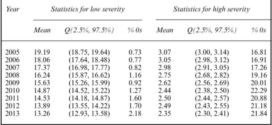
Around 199000 accidents occurred in England in the year 2005 with a decrease down to 139 000 accidents in 2013. The majority of them were of low severity—around 85% of the total number of accidents for all years. Table 1 presents the summary statistics of the accidents data at ward level, as used in the analysis.
Traffic count data for the majority of main roads in England (motorways and A-roads) were obtained from the Department for Transport (Road Traffic Statistics Branch). These are very stable across all the years that were considered in the study (2005–2013), and hence traffic counts based on the middle year, 2009, were used for the analysis. The annual average daily flow
Table 1. Summary statistics of the data at ward level by severity and year in England
Year Statistics for low severity Statistics for high severity
Mean Q(2.5%, 97.5%) % 0s Mean Q(2.5%, 97.5%) % 0s 2005 19.19 (18.75, 19.64) 0.73 3.07 (3.00, 3.14) 16.81 2006 18.06 (17.64, 18.48) 0.77 3.05 (2.98, 3.12) 16.91 2007 17.37 (16.98, 17.77) 0.82 2.98 (2.91, 3.05) 17.26 2008 16.24 (15.87, 16.62) 1.16 2.75 (2.68, 2.82) 19.16 2009 15.63 (15.26, 15.99) 0.92 2.62 (2.56, 2.69) 20.01 2010 14.87 (14.52, 15.22) 1.27 2.44 (2.38, 2.50) 22.29 2011 14.53 (14.18, 14.87) 1.60 2.50 (2.44, 2.57) 20.88 2012 13.89 (13.55, 14.22) 1.70 2.49 (2.43, 2.55) 21.18 2013 13.26 (12.93, 13.58) 2.18 2.35 (2.30, 2.41) 21.84
data, consisting of traffic counts (980 and 16 941 for respectively motorways and A-roads) for each junction-to-junction link on the major road network, were joined within a geographical information system to the Ordnance Survey Meridian road network. The traffic data were joined to the road network by associating points to the correct road links based on road names or, if not available, by associating point to the nearest road link based on distance. In the few occasions when no traffic count was provided for the road link, an estimate was made by calculating the average of the traffic counts of the bordering road segments (Eeftenset al., 2012; de Hoogh
et al., 2013; Beelenet al., 2013).
The resulting road traffic geographical information system file was subsequently intersected with the wards 2001 geography and the traffic volume (or intensity) of each individual intersected road segment was calculated by multiplying the length of the road segment by the annual average daily flow AADF. The total traffic volume at the ward level was then calculated by summing the traffic volumes of all road segments lying within the ward:
TVw=
rs∈w
TVrs
TVrs=length.rs/AADFrs
where TV is the traffic volume, w represents the ward level and rs represents the road segment.
3. Statistical framework
The analysis is carried out within a Bayesian hierarchical framework. We specified a formula-tion which includes spatial and temporal random-effect components. The spatial component consists of spatially structured random effects that allow information to be shared between areas, accounting for any potential spatial correlations, as well as spatially unstructured random effects that account for heterogeneity. The temporal component is structured across time, accounting for potential time correlations. We do not include a heterogeneity term in the temporal component, as the number of time points is relatively small.
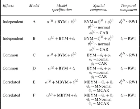
Using this formulation as a baseline, we present a series of models under various assumptions regarding the spatial and temporal dependences between low and high accident severities (Table 2). The models are classified into three main groups according to the type of spatial dependences between the two severities:independentspace effects assume independence between the spatial
Table 2. Models under different assumptions for space and time dependences between severities of accident
Effects Model Model Spatial Temporal
specification component component
Independent A α.j/+BYM+δt.j/ BYM=θ.j/i +φ.j/i δt.j/∼RW1
θ.j/i ∼normal
φ.j/i ∼CAR
Independent B α.j/+BYM+δt BYM=θ.j/i +φ.j/i δt∼RW1
θ.j/i ∼normal
φ.j/i ∼CAR
Common C α.j/+BYM+δt.j/ BYM=θi+φi δt.j/∼RW1
θi∼normal
φi∼CAR
Common D α.j/+BYM +δt BYM=θi+φi δt∼RW1
θi∼normal
φi∼CAR
Correlated E α.j/+MBYM+δt.j/ MBYM=Θi+Φi δt.j/∼RW1
Θi∼MNormal
Φi∼MCAR
Correlated F α.j/+MBYM+δt MBYM=Θi+Φi δt∼RW1
Θi∼MNormal
Φi∼MCAR
Table 3. Hierarchy of the models
Model Spatially structured Spatially unstructured Temporal
effects effects effects
θ.j/i θi Θi φi.j/ φi Φi δ.j/t δt A B C D E F
structure of low and high severities,commonspace effects assume the same spatial structure for the two severities andcorrelatedspace effects assume a certain degree of dependence in the spatial random effects. In all groups we include a temporal dependence via a random walk either common or specific for the levels of severity.
Table 3 shows how the effects are introduced, to help to understand the hierarchy. We describe the groups in detail in the rest of this section.
3.1. Independent space effects
two levels of accident severities (model A in Table 2), as each parameter in the model is severity specific (low and high).
In the first level of the hierarchy, the observed counts of accidentsYit.j/are modelled as
Yit.j/∼Poisson.λ.j/it Offi/, .1/ for wardi, time pointtand severityj. There areN=7932 wards andT=9 time points which correspond to the years 2005, 2006,: : :, 2013. The level of severity is low or high ifj=1 orj=2 respectively. The accident rate is denoted byλ.j/it and the offset variable by Offi, which here is taken as the traffic volume described in Section 2.
The second level of the hierarchy models the accident rateλ.j/it . It is a function of a spatially unstructured componentθ.j/i , a spatially structured componentφ.j/i and a temporally structured componentδt.j/. It also includes a severity-specific interceptα.j/:
log.λ.j/it /=α.j/+θ.j/i +φ.j/i
BYM.j/
+δt.j/: .2/
In the third level, an exchangeable prior is assigned to the spatially unstructured random effects: θ.j/i ∼N.0,σθ2.j// .3/ whereσ2θ.j/is the corresponding variance.
The spatially structured random effectsφ.j/i are assigned a CAR prior (Besag, 1974): φ.j/i |φ.j/.−i/∼N ¯ φ.j/i ,σ 2.j/ φ ni , φ¯.j/i = k∈Diφ .j/ k ni : .4/
Here,σ2φ.j/is the variance for the spatially structured random effects, andφ.j/.−i/denotes all the elements of the vectorφ.j/except for the areai.Direpresents the set of areas that are adjacent to areai(neighbours) andniis the total number of those areas. Hence, the spatially structured random effects follow a normal distribution with a conditional mean given by the average of the neighbouring random effects and conditional variance inversely proportional to the number of neighbouring areas. This results in a spatial smoothing, as information is borrowed across neighbouring areas. The convolution prior for the spatial random effects (BYM =θi+φi) was intially introduced by Besaget al. (1991).
For the temporal component δt.j/ a normal random-walk prior of order 1, RW1, is used. To implement this, we use the temporal analogue of the CAR prior which defines temporal neighbouring points oftast−1 andt+1. Similar to the spatial CAR prior, the underlying as-sumption is a structure where the neighbouring time points are assumed to be similar (Fahrmeir and Lang, 2001; Liet al., 2012).
This prior is defined as
δt.j/|δ.j/.−t/∼ ⎧ ⎪ ⎪ ⎪ ⎨ ⎪ ⎪ ⎪ ⎩ N.δ.j/t+1,σδ2.j//, fort=1, N δt−.j/1+δt+.j/1 2 , σ2.j/ δ 2 , fort=2, 3,: : :, 8, N.δ.j/t−1,σδ2.j//, fort=9, .5/
whereδ.−t/.j/ denotes all elements ofδ.j/except for the time pointtandσδ2.j/denotes the variance in the temporal effects for accidents of severityj.
Kelsall and Wakefield (1999) and used by Wakefieldet al. (2000). Simulation studies showed that this is more appropriate for epidemiological studies when compared with the widely used gamma(0.001, 0.001) and gamma(0.2, 0.0001) priors. This prior distribution plays a minimal role in the posterior distribution and can be described as vague, flat or non-informative (Gelman
et al., 2003). This hyperparameter controls for the extra Poisson variation due to heterogeneity between areas.
Similarly, a gamma(0.5, 0.0005) prior is also assigned to the precisionsτ2.j/
φ = 1=σφ2.j/andτδ2=
1=σδ2.j/, controlling for the variations conditionally on the neighbouring spatial and temporal points respectively. To ensure identifiability of the model, we imposed sum to 0 constraints on the vectorsφandδand a flat prior for the interceptα.
In the group of independent space effects, we also include model B, which differs from model A only in the temporal effectsδt∼RW1, which in this case are taken to be common between the two severities.
3.2. Common space effects
Following the Poisson log-normal specification that is described in equations (1)–(5), we present two additional models that assume the same spatial effect for accidents of low and high level of severity. This is included in the model in the form of a common distribution (not severity spe-cific). The spatially unstructured effectsθiare assigned a common normal distribution and the spatially structured effectsφi are assigned a common CAR distribution. This means dropping thej-superscript in equations (3) and (4). The temporal random effects are specified either as in-dependent (model C) or common (model D). The prior specification is the same as in Section 3.1.
3.3. Correlated space effects
Finally, we extend the BYM specification to the multivariate BYM (MBYM) model which con-siders a multivariate setting across severities for both spatially structuredφi- and unstructured θi-effects quantifying their correlation.
The spatially structured effectsφifollow a multivariate CAR (MCAR) prior. Assuming that we have a two-dimensional vector of spatially structured random effectsΦi=.Φi1,Φi2) for each
areai=1,: : :,N, where the subscripts 1 and 2 represent low and high severity respectively, then we extend the CAR specification as follows:
Φi|Φ.−i/∼N.Φ¯i,ΣΦ=ni/, Φ¯i=.Φ¯i1,Φ¯i2/, Φ¯ip=
k∈DiΦkp
ni , p=1, 2: .6/ Φ.−i/=.Φ1.−i/,Φ2.−i// denotes the elements of the matrixΦexcluding the area i. As in the
univariate CAR case, Di and ni are the set of areas adjacent to areai and the number of those areas respectively.ΣΦis the 2×2 covariance matrix with diagonal elementsσ2.1/
φ andσ2.
2/
φ
representing the conditional variances for each level of severity. The within-area conditional correlation of random effects of low and high severity ρφ is modelled via the off-diagonal terms ΣΦ= σ2.1/ φ ρφσ.φ1/σ.φ2/ ρφσφ.1/σφ.2/ σφ2.2/ :
Hence, the MCAR model not only takes into account the spatial correlation between areas for each severity but also allows for correlation between severities in each spatial unit.
Also, for each areai=1,: : :,N we have a two-dimensional vector of spatially unstructured random effectsΘi=.Θi1,Θi2) where again the subscripts 1 and 2 represent low and high severity
respectively. On these, a multivariate normal distribution is defined as
Θi∼MVN.0,ΣΘ/ .7/
where0is a 1×2 vector andΣΘis a 2×2 covariance matrix ΣΘ= σ2.1/ θ ρθσθ.1/σθ.2/ ρθσ.θ1/σ.θ2/ σ2. 2/ θ
with diagonal elementsσ2θ.1/ andσθ2.2/ representing the conditional variances for each severity, whereas the off-diagonal elementsρθmodel the within-area conditional correlation of random effects of low and high severity. In addition toρφandρθ, we also estimateρtotwhich is the
within-area conditional correlation for the total random effect (i.e. the sum of spatially structured and unstructured components).
The precision matrixΩΦ=Σ−Φ1is assigned a Wishart.A,k/prior whereAandkdenote the inverse scale matrix and the degrees of freedom respectively. We setk=2 for a weakly infor-mative specification. For the inverse scale matrixA, typically a prior belief of the value of the covariance matrix is used. We set the entries on the diagonals to 500 and the off-diagonal entries to 0.0005, following Kass and Natarajan (2006), who suggested considering the data on the prior specification in the multivariate case, and Gelman (2006), who recommended taking con-siderable care with the prior specification on unobserved parameters and assigning reasonable values in advance. Although such external information does not usually bias the main estimates, it may have some influence on the precision of the estimates, and it is important to explore this through sensitivity analysis.
Similarly to the spatially structured case, a Wishart.A,k/prior is assigned to the precision matrixRΘ=Σ−Θ1, with the same parameterskandA. The prior specifications for the remaining components are as defined in Section 3.1.
The MBYM specification that is described in this section, where MBYM=Φi+Θi, is then coupled with independent time effectsδ.j/t in model E and common time effectsδtin model F.
3.4. Spatial fraction
For all the models, we are interested in estimating the relative contribution of structured and unstructured effects to the overall variability. We quantify this through the fraction of the marginal variability of the structured random effects σφ2, over the total marginal variability σ2
θ+σ2φ. The parameterσφ2is not directly available since, from their definition, the spatial effects
ofφiare conditional on the neighbouring effects. We thus use the conditional variance which is available, to estimate the empirical marginal variance ˆσ2φ=Σi.φi− ¯φ/2=.n−1/. The spatial fraction of interest is given by
fracφ= σˆ 2 φ σ2 θ+σˆ2φ :
When the spatial fraction is close to 1, structured effects explain most of the variability of the model, whereas when this is close to 0 the unstructured random effects dominate.
3.5. Model comparison and checking
In this work we use the deviance information criterion (DIC) (Spiegelhalteret al., 2002) to carry out comparisons between the various models that we develop, but we stress that this is solely
used for building the models to find the most suitable for the data at hand, and it is not intended as an absolute measure.
The DIC has been extensively used for comparisons between hierarchical models in which the number of parameters is not clearly defined. This is a generalization of Akaike’s informa-tion criterion, as it trades off model fit against a measure of complexity. Similarly to Akaike’s information criterion, lower values indicate better performance.
Although the DIC is a useful tool for comparisons between different models, it does not give any information about whether a specific model is adequate. To assess this, we use posterior predictive checks and Bayesianp-values, as suggested by Lunnet al. (2012). We generate a predictive distribution of accident countsYrep for each level of severity, year and area under each model specified in Table 2 and then compare these predictions with the observed data. If the model fits the data adequately, the replicated data should look similar to the observed data. In addition to this graphical check, we also calculate a Bayesianp-value which gives the predictive probability of obtaining an extreme result:
pBayes=Pr{T.Yrep,λ/ > T.Y,λ/|Y}:
T.Y,λ/is a test statistic, and here we use the common choice ofT.Y,λ/=YandT.Yrep,λ/=Yrep to check for individual outliers. ApBayes-value close to 0.5 suggests that the generated data are
compatible with the model, whereas values close to 0 and 1 are considered extreme and hence suggest poor fit.
Finally, a sensitivity analysis is conducted to evaluate how robust the posterior estimates are under the probability model that is specified by using different priors. In the models with a CAR distribution in the spatially structured effects (independent and common space effects), the prior distribution for the precisionsτφ was changed to a half-Cauchy distribution on the natural scale of standard deviation as recommended by Gelman (2006):σφ∼z=√γ, whereσφ is Cauchy distributed with location 0 and scaleB, which in turn is assigned a non-informative uniform distribution. In the models with an MCAR distribution (correlated space effects), the diagonals of the Wishart distribution on the multivariate normal and MCAR priors are changed to 1 and 1000, whereas the off-diagonals remain 0.0005.
3.6. Posterior distribution of accident rates
Typically in disease mapping, the results of the analysis are presented in the form of maps that display posterior mean relative risks (or accident rates in the context of road traffic accidents) across areas. This allows us to visualize spatial patterns of risk, and also to assess the degree of smoothing by comparing those against maps of crude rates.
Since the posterior mean rates do not make full use of the output of Bayesian analysis, several researchers have proposed to map the probability that a rate exceeds a specified threshold (Clayton and Bernardinelli, 1992; Richardsonet al., 2004). This is a more powerful tool, which takes into account the uncertainty in the posterior estimates, thus highlighting areas that are characterized by strong evidence of an increased risk.
In this paper, besides mapping the posterior accident ratesλ.j/it , we want to highlight dangerous areas; thus we adapt the posterior probability maps to fit this purpose. We borrow ideas from the concept of ranking, which is extensively used in road traffic accidents analysis (Christiansen
et al., 1992; Schl ¨uteret al., 1997; Miranda-Morenoet al., 2005; Aguero-Valverde and Jovanis, 2007) and calculate the posterior probability that the spatial component of the accident rates (exp(θi+φi)) is ranked among the top 800, accounting for roughly 10% of the total number of areas (7932), for each severity levelj. This is given by
Pr[rank{exp.θi+φi/.j/}<800]:
In addition, we compare the rank order of areas based on crude rates (averaged across years), against the rank order of areas under the model to highlight potential differences and evaluate the effect of the modelling approach. To estimate the latter, we use the posterior mean of the rank (Miaou and Song, 2005; Tunaru, 2002) of the spatial component (exp.θi+φi//.
4. Results
All models are implemented in OpenBUGS. Two chains are run for each parameter for each model with different initial values for around 50000 iterations depending on the complexity of the model, from which 5000–10000 are discarded as a burn-in, and estimates are based on the remaining samples. The simulations took between 20 and 27 h per model on an Intel Core processor at 3.40 GHz with 8 Gbytes of random-access memory. The convergence diagnostics that we used include a visual check of trace plots, the Brooks–Gelman–Rubin statistic, auto-correlation plots and Monte Carlo error which should be less than 5% of the posterior standard deviation.
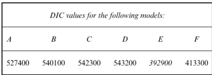
Analysing the DIC values of the models in Table 4 allows us to make several observations regarding their fit to the road traffic accidents data. In general, comparing models within groups, it is clear that those with independent temporal effects are favoured over those with common temporal effects (model A better than model B, model C better than model D, and model E better than model F).
Regarding the spatial effects, which are of primary interest in this paper, it is shown that common space effects provide the worst fit, with high relative differences in the DIC than independent space effects that follow.
The benefit of including a multivariate structure in the spatial effects (the MBYM specifica-tion) can be seen in the correlated space effects, where the DIC decreased greatly. This indicates that there is a non-negligible correlation between low and high severities, in both spatially structured and unstructured effects, which needs to be considered in the model. We have also developed a model with a multivariate structure either inφior inθi alone, followed by an in-dependent structure in the other parameter, to investigate the complex structure of the data further. However, these models did not provide any important improvement, indicating that it is the synergy of the multivariate structure onφiandθithat best supports the data. In addition, the fact that model E is favoured over model F suggests that there are differences in the temporal trends between low and high severities over the period 2005–2013.
Table 5 reports the parameter estimates of all the models that are considered in this study. In general, we observe that most of the estimates are consistent among the different models.
Table 4. DIC values for competing models† DIC values for the following models:
A B C D E F
527400 540100 542300 543200 392900 413300
†A, B, independent effects models; C, D, common effects models; E, F, correlated effects models. The best model is shown in italics.
Ta b le 5 . Mean estimates fo r par ameters of all models de v eloped in the study † Estimates fo r the follo wing models: ABCD E F Lo w High Lo w High Lo w High Lo w High Lo w High Lo w High se verity se verity se verity se verity se verity se verity se verity se verity se verity se verity se verity se verity Inter cept exp( α ) 0.192 0.032 0.192 0.032 0.196 0.033 0.196 0.033 0.192 0.033 0.192 0.033 ( < 0.001) ( < 0.001) ( < 0.001) ( < 0.001) ( < 0.001) ( < 0.001) ( < 0.001) ( < 0.001) ( < 0.001) ( < 0.001) ( < 0.001) ( < 0.001) V ariances 2σθ 0.089 0.159 0.095 0.157 0.105 0.316 0.414 0.415 0.411 0.413 (0.011) (0.014) (0.012) (0.013) (0.012) (0.018) (0.011) (0.011) (0.011) (0.011) ˆ σ 2 φ 0.854 0.630 0.850 0.630 0.790 0.795 0.641 0.534 0.647 0.537 (0.014) (0.017) (0.014) (0.016) (0.013) (0.013) (0.013) (0.013) (0.014) (0.014) σ 2 σ 0.0028 0.0028 0.0026 0.0027 0.0028 0.0027 0.0028 0.0028 0.0027 (0.002) (0.002) (0.002) (0.002) (0.002) (0.002) (0.002) (0.002) (0.002) Corr elations ρφ ———— 0.769 0.772 (0.009) (0.009) ρθ ———— 0.643 0.641 (0.010) (0.010) ρtot ———— 0.740 0.0741 (0.007) (0.0007) Spatial fr action fr acφ 0.906 0.797 0.900 0.801 0.883 0.716 0.646 0.602 0.650 0.606 (0.012) (0.017) (0.013) (0.017) (0.013) (0.014) (0.009) (0.010) (0.009) (0.010) †A, B , independent ef fects models; C , D , common ef fects models; E, F , corr ela ted ef fects models . Standar d d evia tions ar e in par entheses .
The overall mean accident rate is around 0.19 for low severity and 0.03 for high severity. As expected, some differences in the variances for the spatially structured and unstructured effects exist between the models of different groups. More specifically, the independent space effects give an average of 0.85 and 0.63 for the variability inφi for low and high severity respectively, whereas this is somewhere between the two values under the common space effects models. The same stands for the variability inθi. Under the correlated space effects models, the variability inφi decreases by around 0.8 for low severity and 0.3 for high severity, whereas, at the same time, the variability inθi increases by around 0.3 for both severities, which is important if we consider the small standard deviations associated with these estimates. Potentially, this is because part of the unstructured variabilityσ2θ in the data can only be captured under a multivariate specification. The effect of including a multivariate setting for bothφiandθiis also notable in the reduction in uncertainty associated with the variance estimates due to the information that is borrowed between the two severities. The larger uncertainty in the independent case is due to the correlation between severities which is not taken into account in the model. The spatial fraction changes across groups of models as this is calculated on the basis of the variances, with the estimates becoming slightly more precise under correlated space effects.
Within the correlated effects group of models, and by looking at the temporal effectsσδ, we observe that their magnitude seems to be the same for low and high severities; however, as model E is favoured over model F, different patterns in the temporal trend between the two severities are suggested.
Focusing on the preferred model (model E) in Table 5, we draw conclusions regarding the sources of variability in road traffic accidents data. A comparison of ˆσ2φandσ2
θ indicates that
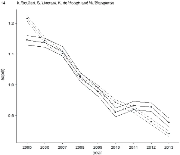
the spatially structured effects are somewhat stronger than the spatially unstructured effects for both low and high severities. This can also be seen by the values of the spatial fraction fracφ. This is distributed around 0.646 for accidents of low severity, and 0.602 for accidents of high severity, indicating that, although the effect of spatially structured effects is stronger in both categories, the unstructured effects are also non-negligible. The conditional within-area correlations forφi andθi are 0.77 and 0.64 respectively, whereas the corresponding correlation due to the total random effects is 0.74. Fig. 1 presents the temporal effects on the exponential scale, showing an overall decrease in the posterior rates across years. Although for low severity an almost linear pattern is observed, for high severity the downward trend becomes flatter after 2010. What we learn from these findings is that the present data have a complex structure as the variation is due to several sources of variability; spatially structured, spatially unstructured and temporal random effects, as well as the correlation between severities are needed to explain this.
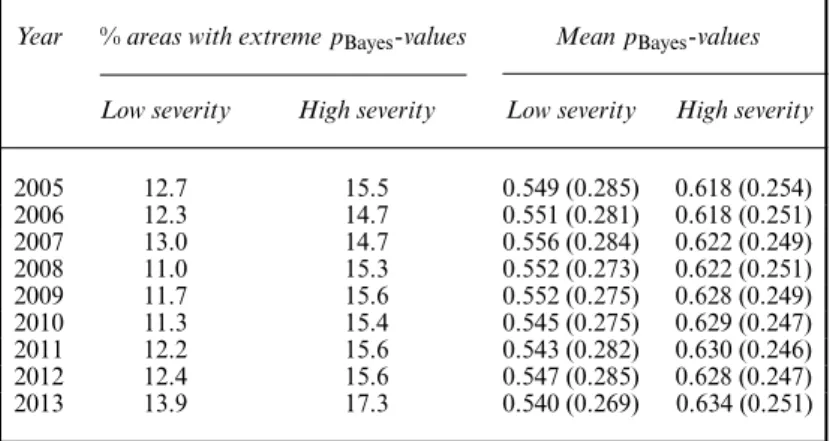
Table 6 shows the proportion of areas with extreme pBayes-values for each year and level
of severity, and the mean values under model E. An adequate model fit is suggested, as only 13–17% of areas are assigned extremepBayes-values, and these are close to 0.5, varying from
0.55 to 0.63. This is also confirmed by maps ofpBayes-values which can be found in Fig. 3 of the
on-line supporting material.
Sensitivity analyses performed did not highlight noticeable differences on the spatial compo-nentθi+φias well as on the temporal component, as seen in Figs 4 –7 in the on-line supporting material, suggesting that our results are robust to the model specification.
We produce maps which help to visualize how the risk of road traffic accidents is distributed across space. Figs 2(a) and 2(b) show crude rates calculated for a specific year (2005), for low and high severity, together with the corresponding posterior rates under model E (Figs 2(c) and 2(d)).
First, comparing crude and posterior mean rates for high severity, we observe that these are greatly smoothed out under the model. The map of crude rates in Fig. 2(b) does not indicate
Fig. 1. Median values and 25th and 75th percentiles for the temporal effects under model E:
, high severity; , low severitya particular pattern of risk, showing fairly similar effects across the south-west, central and central-east of England. The corresponding map of posterior rates in Fig. 2(d) uncovers a clear pattern; the effects in the south-west are eliminated, whereas these become stronger towards the eastern part of England and even stronger in the north, mainly in the area that includes Liverpool, Manchester, Leeds and Sheffield, as well as along the southern coast. Clusters of dangerous areas are now detected in the region of Southend-on-Sea, and around Hull and Bridlington. This is in line with common knowledge, as the road connecting those (the A165 road) is believed to be the most dangerous in the East Riding. Interestingly, motorways across England can also be clearly distinguished in Fig. 2(d). To illustrate this, we have linked the map in Fig. 2(d) with the motorway network within the geographical information system and the resulting map can be seen in the on-line supporting material. It appears that the wards including motorways, e.g. the M24, M1, M4 and M11 motorways, show low posterior rates compared with the surrounding regions. This is obvious even in central London, where the inner part suffers most and, moving outside, the wards including motorways become less risky. The high accident rates within London and other big cities can be explained by the high numbers of pedestrians and cyclists who are involved in those, whereas the high rates in areas between big cities can be explained by the excess speed of vehicles and road conditions that lead to severe
Table 6. Proportion of areas with extremepBayes-values and the mean
pBayes-values for low and high severity under model E†
Year %areas with extremepBayes-values MeanpBayes-values
Low severity High severity Low severity High severity
2005 12.7 15.5 0.549 (0.285) 0.618 (0.254) 2006 12.3 14.7 0.551 (0.281) 0.618 (0.251) 2007 13.0 14.7 0.556 (0.284) 0.622 (0.249) 2008 11.0 15.3 0.552 (0.273) 0.622 (0.251) 2009 11.7 15.6 0.552 (0.275) 0.628 (0.249) 2010 11.3 15.4 0.545 (0.275) 0.629 (0.247) 2011 12.2 15.6 0.543 (0.282) 0.630 (0.246) 2012 12.4 15.6 0.547 (0.285) 0.628 (0.247) 2013 13.9 17.3 0.540 (0.269) 0.634 (0.251)
†Standard deviations are in parentheses.
and fatal accidents. Other areas that are shown to be prone to accidents of high severity are countryside areas, such as Northumberland and the North York, Peak District and Yorkshire Dales national parks, where road conditions and characteristics (narrow roads, bends, slopes, etc.) might be an exlanation for this.
Second, looking at the posterior mean rates for low severity in Fig. 2(c), we can see that urban areas in England appear to be more dangerous. The risk for accident incidence is focused mainly within big cities, with central London showing a significantly increased risk. Other big cities, such as Newcastle, Birmingham, Liverpool, Leeds, Sheffield and Manchester, are also shown to be dangerous. This could be again due to the high numbers of pedestrians and cyclists, and the presence of bus and cycle lanes.
In contrast with high severity, there are no obvious differences between maps of crude and posterior rates when comparing Figs 2(a) and 2(c). The fact that the model does not affect the rates for low severity importantly is reasonable if we consider that these consist of high counts in general, and the model is designed to provide smoothing to low counts that suffer from great variability. The information of low severity in the model yet contributes to stable estimates for high severity, and this is one of the main aspects of this paper; strength is borrowed, not only between areas, but also between levels of severity.
Moreover, the probability maps in Fig. 3 help to discriminate specific areas of excess risk in England and focus on those which show strong evidence of increased risk, after accounting for the uncertainty in the posterior estimates. The west, east and north-east parts of England are no longer shown as dangerous, and clusters of areas that consistently belong to the top 800 ranked areas are observed in central London, and in the area around Southend-on-Sea. This gives a clearer picture of the most dangerous areas at a national level, and therefore provides evidence for prioritizing interventions to reduce rates.
Finally, by comparing ranks that are generated under the model against ranks under crude rates for the top 100 areas (Fig. 4), we observe that for low severity these are quite consistent, whereas, for high severity, they differ importantly. Among the top 100 ranked areas the pro-portion of those that have a difference of more than 15 places between the two ranking criteria is 0.02% for low severity and 0.26% for high severity; when we consider the top 800 ranked areas these numbers increase to 0.27% and 0.75% respectively, suggesting that the features of the model have an important influence on the results.
< 0. London London London London 1 0. 1 - 0.25 0. 25 - 0 .5 > 0. 5 < 0.01 0. 01 - 0. 03 0. 03 - 0. 07 > 0.07 < 0. 1 0. 1 - 0.25 0. 25 - 0 .5 > 0. 5 < 0.01 0. 01 - 0. 03 0. 03 - 0. 07 > 0.07 (a) (c) (b) (d)
Fig. 2. (a), (b) Crude and (c), (d) posterior accident rates for a specific year for (a), (c) low and (b), (d) high severity
(a) (b)
London
London
Fig. 3. Probability that residual accident rates belong to the top 800 ranked areas for (a) low and (b) high severity: , less than 0.2; , 0.2–0.8; , greater than 0.8
(a) (b)
Fig. 4. Area ranks based on crude ratesversusposterior ranks for the top 100 areas: (a) low severity; (b) high severiy
5. Discussion
In this paper we have compared models for road traffic accidents data under various assumptions on the spatial and temporal dependences between severities. These models combine ideas from
a Bayesian hierarchical framework with space–time effects and multivariate analysis to produce a flexible framework for the analysis of road traffic accidents by level of severity.
We have identified the MBYM model as the most appropriate in this context. This model consists of both multivariate spatially structured and unstructured effects that assume a degree of correlation in the respective components between severities, allowing at the same time the quantification of this correlation. The results suggest a high correlation between severities in both spatially structured and unstructured effects, whereas the time effects are better modelled via separate components indicating fairly different trends for the two severities.
From the point of view of policy making, probability maps and rankings are used to aid the detection of areas that are characterized by excess risk. One of the strengths of our model is that it not only provides top ranked areas based on the mean rates of accidents, but in ad-dition it takes into account the uncertainty associated, providing policy makers with a high level of information to draw priority plans for actions. We have shown that this could greatly influence high severity accidents, owing to the small numbers. For example, the results of our analysis can be used centrally to decide where to allocate funding to decrease the number of injuries and fatalities due to road accidents. Among the policies that can be implemented to prevent road traffic accidents in the most high-risk areas, there are environmental changes (such as the introduction of speed cameras, or marked pathways for cyclists) and safety ed-ucation and skills training (such as road safety media campaigns or providing free safety equipment). Different policies can be used for high-risk areas for high and low severity ac-cidents.
The paper has shown that the MBYM specification offers a great improvement over other model specifications that consider joint modelling of accidents by level of severity; however, as always the case with disease mapping models we should treat this as an explorative analysis, aiming solely at investigating the spatial and temporal pattern of accidents and at identifying areas that are characterized by particularly high risks. We stress that we are not placing our-selves in the context of hot spot analysis, which involves a deep investigation from identifying the dangerous locations, ranking these locations according to various criteria and providing explanations of why certain locations are hot spots, and which usually consider information on the cost of the accidents (Miaou and Song, 2005; Brijs et al., 2007). Instead, our mod-elling approach can serve as a first step for policy making, which should be followed by further investigation.
The next step of this research would be to assess risk factors formally, including these in the model as explanatory variables. For instance socio-economic and demographic factors and adverse weather conditions could be good candidates to explain the pattern that is seen for slight and severe accidents. It would be important to consider also the type of road (i.e. major or minor) and other characteristics, and particularly whether a ward includes a motorway or not, to investigate formally the findings that were suggested by the current analysis. In addition, information on the classification of an area as rural, suburban or urban can be incorporated in the model.
Aiming at identifying clusters of areas with an unusual road accidents pattern (e.g. increasing in time whereas the general temporal trend shows a decrease) more complex models including an interaction term could be considered, which would provide information on area changes across space and time jointly as presented in Liet al. (2012). However, this type of models entails a considerable computational burden for large study regions such as the whole of England; thus we decided against it in the present paper as we were interested in investigating the spatiotemporal trend of accidents for the entire study region. A natural extension of this paper would be to focus on some specific regions, e.g. around the big cities showing evidence of increased risk, and
to go more deeply into these by means of a more complex model which considers for instance a mixture specification on the interactions.
Acknowledgements
Areti Boulieri acknowledges support from the National Institute for Health Research and the Medical Research Council Doctoral Training Partnership. Marta Blangiardo acknowledges sup-port from the National Institute for Health Research and the Medical Research Council–Public Health England Centre for Environment and Health. Silvia Liverani acknowledges support from the Leverhulme Trust (grant ECF-2011-576).
References
Ackaah, W. and Salifu, M. (2011) Crash prediction model for two-lane rural highways in the Ashanti region of
Ghana.IATSS Res.,35, 34–40.
Aguero-Valverde, J. (2011) Direct spatial correlation in crash frequency models.3rd Int. Conf. Road Safety and
Simulation, Indianapolis.
Aguero-Valverde, J. and Jovanis, P. (2006) Spatial analysis of fatal and injury crashes in Pennsylvania.Accidnt
Anal. Prevn,38, 618–625.
Aguero-Valverde, J. and Jovanis, P. P. (2007) Identifying road segments with high risk of weather-related crashes
using full Bayesian hierarchical models.86th A. Meet. Transportation Research Board, Washington DC.
Aguero-Valverde, J. and Jovanis, P. (2009) Bayesian multivariate Poisson lognormal models for crash severity
modeling and site ranking.J. Transportn Res. Bd,2136, 82–91.
Al-Osh, M. A. and Alzaid, A. A. (1987) First-order integer-valued autoregressive (INAR(1)) process.J. Time Ser.
Anal.,8, 261–275.
Beelen, R., Hoek, G., Vienneau, D., Eeftens, M., Dimakopoulou, K., Pedeli, X., Tsay, M.-Y., K ¨unzli, N., Schikowski, T., Marcon, A., Eriksen, K. T., Raaschou-Nielsen, O., Stephanou, E., Patelarou, E., Lanki, T., Yli-Tuomi, T., Declercq, C., Falq, G., Stempfelet, M., Birk, M., Cyrys, J., von Klot, S., N´ador, G., Varr, M. J., D´edel´e, A., Grauleviien, R., M ¨olter, A., Lindley, S., Madsen, C., Cesaroni, G., Ranzi, A., Badaloni, C., Hoff-mann, B., Nonnemacher, M., Kr¨amer, U., Kuhlbusch, T., Cirach, M., de Nazelle, A., Nieuwenhuijsen, M., Bellander, T., Korek, M., Olsson, D., Str ¨omgren, M., Dons, E., Jerrett, M., Fischer, P., Wang, M., Brunekreef, B. and de Hoogh, K. (2013) Development of NO2 and NOx land use regression models for estimating air
pollution exposure in 36 study areas in Europe—the ESCAPE project.Atmosph. Environ.,72, 10–23.
Bernardinelli, L., Clayton, D., Pascutto, C., Montomoli, C., Ghislandi, M. and Songini, M. (1995) Bayesian
analysis of space-time variation in disease risk.Statist. Med.,14, 2433–2443.
Besag, J. (1974) Spatial interaction and the statistical analysis of lattice systems (with discussion).J. R. Statist.
Soc.B,36, 192–236.
Besag, J., York, J. and Molli´e, A. (1991) Bayesian image restoration, with two applications in spatial statistics. Ann. Inst. Statist. Math.,43, 1–20.
Best, N., Richardson, S. and Thomson, A. (2005) A comparison of Bayesian spatial models for disease mapping. Statist. Meth. Med. Res.,14, 35–59.
Bijleveld, F. D. (2005) The covariance between the number of accidents and the number of victims in multivariate
analysis of accident related outcomes.Accidnt Anal. Prevn,37, 591–600.
Bijleveld, F., Commandeur, J., Koopman, S. J. and van Montfort, K. (2010) Multivariate non-linear time series
modelling of exposure and risk in road safety research.Appl. Statist.,59, 145–161.
Box, G. E. and Jenkins, G. M. (1976)Time Series Analysis: Forecasting and Control, revised edn. San Francisco:
Holden-Day.
Brijs, T., Karlis, D., Van den Bossche, F. and Wets, G. (2007) A Bayesian model for ranking hazardous road sites. J. R. Statist. Soc.A,170, 1001–1017.
Christiansen, C., Morris, C. and Pendleton, O. (1992) A hierarchical Poisson model with beta adjustments for
traffic accident analysis.Technical Report 103. Center for Statistical Sciences, University of Texas at Austin,
Austin.
Clayton, D. and Bernardinelli, L. (1992) Bayesian methods for mapping disease risk. InGeographical and
Envi-ronmental Epidemiology: Methods for Small Area Studies(eds P. Elliott, J. Cuzick, D. English and R. Stern).
Oxford: Oxford University Press.
Department for Transport (2010) Road Accident Statistics Branch, road accident data, 2009.Technical Report.
UK Data Archive, Colchester.
Durbin, J. and Koopman, S. J. (2012)Time Series Analysis by State Space Methods. Oxford: Oxford University
Eeftens, M., Tsai, M.-Y., Ampe, C., Anwander, B., Beelen, R., Bellander, T., Cesaroni, G., Cirach, M., Cyrys, J., de Hoogh, K., Nazelle, A. D., de Vocht, F., Declercq, C., D´edel´e, A., Eriksen, K., Galassi, C., Graˇzuleviˇcien´e, R., Grivas, G., Heinrich, J., Hoffmann, B., Iakovides, M., Ineichen, A., Katsouyanni, K., Korek, M., Kr¨amer, U., Kuhlbusch, T., Lanki, T., Madsen, C., Meliefste, K., M ¨olter, A., Mosler, G., Nieuwenhuijsen, M., Oldenwening, M., Pennanen, A., Probst-Hensch, N., Quass, U., Raaschou-Nielsen, O., Ranzi, A., Stephanou, E., Sugiri, D., Udvardy, O., Vask ¨ovi, E., Weinmayr, G., Brunekreef, B. and Hoek, G. (2012) Spatial variation of PM2.5, PM10, PM2.5 absorbance and PMcoarse concentrations between and within 20 European study areas and the
relationship with NO2—results of the ESCAPE project.Atmosph. Environ.,62, 303–317.
Eksler, V., Lassarre, S. and Thomas, I. (2008) Belgian regions: Federated or divided in road fatality risk evolution?
(Available from http://www.ekf.vsb.cz/export/sites/ekf/projekty/cs/weby/esf-0116/
databaze-prispevku/clanky ERSA 2008/139.pdf.)
Fahrmeir, L. and Lang, S. (2001) Bayesian inference for generalized additive mixed models based on Markov
random field priors.Appl. Statist.,50, 201–220.
Fridstrom, L., Ifver, J., Ingebrigtsen, S., Kulmala, R. and Thomsen, L. K. (1995) Measuring the contribution of
randomness, exposure, weather, and daylight to the variation in road accident counts.Accidnt Anal. Prevn,27,
1–20.
Gaudry, G., Long, R. and Qian, T. (1993) A martingale proof of L2 boundedness of Clifford-valued singular
integrals.Ann. Mat. Pura Appl.,165, 369–394.
Gelman, A. (2006) Prior distributions for variance parameters in hierarchical models (comment on article by
Browne and Draper).Baysn Anal.,1, 515–534.
Gelman, A., Carlin, J. B., Stern, H. S. and Rubin, D. B. (2003)Bayesian Data Analysis. Boca Raton: Chapman
and Hall–CRC.
Ghosh, M., Natarajan, K., Stroud, T. W. F. and Carlin, B. P. (1998) Generalized linear models for small-area
estimation.J. Am. Statist. Ass.,93, 273–282.
Ghosh, M. and Rao, J. N. K. (1994) Small area estimation: an appraisal.Statist. Sci.,9, 55–76.
Goh, B. H. (2005) The dynamic effects of the Asian financial crisis on construction demand and tender price levels
in Singapore.Build. Environ.,40, 267–276.
Graham, D. J. and Glaister, S. (2003) Spatial variation in road pedestrian casualties: the role of urban scale,
density and land-use mix.Urb. Stud.,40, 1591–1607.
de Hoogh, K., Wang, M., Adam, M., Badaloni, C., Beelen, R., Birk, M., Cesaroni, G., Cirach, M., Declercq, C., D´edel´e, A., Dons, E., de Nazelle, A., Eeftens, M., Eriksen, K., Eriksson, C., Fischer, P., Grauleviien, R., Gryparis, A., Hoffmann, B., Jerrett, M., Katsouyanni, K., Iakovides, M., Lanki, T., Lindley, S., Madsen, C., M ¨olter, A., Mosler, G., Ndor, G., Nieuwenhuijsen, M., Pershagen, G., Peters, A., Phuleria, H., Probst-Hensch, N., Raaschou-Nielsen, O., Quass, U., Ranzi, A., Stephanou, E., Sugiri, D., Schwarze, P., Tsai, M.-Y., Yli-Tuomi, T., Varr, M. J., Vienneau, D., Weinmayr, G., Brunekreef, B. and Hoek, G. (2013) Development of
land use regression models for particle composition in twenty study areas in Europe.Environ. Sci. Technol.,47,
5778–5786.
Houston, D. J. and Richardson, L. E. (2002) Traffic safety and the switch to a primary seat belt law: the California
experience.Accidnt Anal. Prevn,34, 743–751.
Jones, A. P., Haynes, R., Kennedy, V., Harvey, I. M., Jewell, T. and Lea, D. (2008) Geographical variations in
mortality and morbidity from road traffic accidents in England and Wales.Hlth Place,14, 519–535.
Jovanis, P. P. and Chang, H.-L. (1986) Modeling the relationship of accidents to miles traveled.J. Transportn Res.
Bd,1068, 42–51.
Kass, R. E. and Natarajan, R. (2006) A default conjugate prior for variance components in generalized linear
mixed models (comment on article by Browne and Draper).Baysn Anal.,3, 535–542.
Kelsall, J. and Wakefield, J. (1999) Discussion of Bayesian models for spatially correlated disease and exposure
data, by Bestet al.Baysn Statist.,6, 151.
Kim, K. and Yamashita, E. (2002) Motor vehicle crashes and land use: empirical analysis from Hawaii.J.
Trans-portn Res. Bd,1784, 73–79.
Knorr-Held, L. (2000) Bayesian modelling of inseparable space-time variation in disease risk.Statist. Med.,19,
2555–2567.
Knorr-Held, L. and Besag, J. (1998) Modelling risk from a disease in time and space.Statist. Med.,17, 2045–2060.
Li, G., Best, N., Hansell, A. L., Ahmed, I. and Richardson, S. (2012) BaySTDetect: detecting unusual temporal
patterns in small area data via Bayesian model choice.Biostatistics,13, 695–710.
Lunn, D., Jackson, C., Best, N., Thomas, A. and Spiegelhalter, D. (2012)The BUGS Book: a Practical Introduction
to Bayesian Analysis. Boca Raton: Chapman and Hall–CRC.
Ma, J. and Kockelman, K. (2006) Bayesian multivariate Poisson regression for models of injury count, by severity. J. Transportn Res. Bd,1950, 24–34.
Ma, J., Kockelman, K. M. and Damien, P. (2008) A multivariate Poisson-lognormal regression model for prediction
of crash counts by severity, using Bayesian methods.Accid. Anal. Prevn,40, 964–975.
MacNab, Y. C. (2004) Bayesian spatial and ecological models for small-area accident and injury analysis.Accid.
Anal. Prevn,36, 1019–1028.
MacNab, Y. C. and Dean, C. B. (2001) Autoregressive spatial smoothing and temporal spline smoothing for
MacNab, Y. C. and Dean, C. B. (2002) Spatio-temporal modelling of rates for the construction of disease maps. Statist. Med.,21, 347–358.
Maiti, T. (1998) Hierarchical Bayes estimation of mortality rates for disease mapping.J. Statist. Planng Inf.,69,
339–348.
Mardia, K. V. (1988) Multi-dimensional multivariate Gaussian Markov random fields with application to image
processing.J. Multiv. Anal.,24, 265–284.
McKenzie, E. (1985) Some simple models for discrete variable time series.Wat. Resour. Bull.,21, 645–650.
Miaou, S. P. (1994) The relationship between truck accidents and geometric design of road sections: Poisson versus
Negative Binomial regressions.Accidnt Anal. Prevn,26, 471–482.
Miaou, S. P. and Lum, H. (1993) Modeling vehicle accidents and highway geometric design relationships.Accidnt
Anal. Prevn,25, 689–709.
Miaou, S. P. and Song, J. J. (2005) Bayesian ranking of sites for engineering safety improvements: decision
pa-rameter, treatability concept, statistical criterion, and spatial dependence.Accidnt Anal. Prevn,37, 699–720.
Miaou, S. P., Song, J. J. and Mallick, B. K. (2003) Roadway traffic crash mapping: a space-time modeling approach. J. Transportn Statist.,6, no. 1.
Miranda-Moreno, L. F., Fu, L., Saccomanno, F. F. and Labbe, A. (2005) Alternative risk models for ranking
locations for safety improvement.J. Transportn Res. Bd,1908, 1–8.
Noland, R. B. and Quddus, M. A. (2004) A spatially disaggregate analysis of road casualties in England.Accidnt
Anal. Prevn,36, 973–984.
Park, E. S. and Lord, D. (2007) Multivariate Poisson lognormal models for jointly modeling crash frequency by
severity.J. Transportn Res. Bd,2019, 1–6.
Qin, X., Ivan, J. N. and Ravishanker, N. (2004) Selecting exposure measures in crash rate prediction for two-lane
highway segments.Accidnt Anal. Prevn,36, 183–191.
Quddus, M. A. (2008a) Modelling area-wide count outcomes with spatial correlation and heterogeneity: an
analysis of London crash data.Accidnt Anal. Prevn,40, 1486–1497.
Quddus, M. A. (2008b) Time series count data models: an empirical application to traffic accidents.Accid. Anal.
Prevn,40, 1732–1741.
Richardson, S., Abellan, J. J. and Best, N. (2006) Bayesian spatio-temporal analysis of joint patterns of male and
female lung cancer risks in Yorkshire (UK).Statist. Meth. Med. Res.,15, 385–407.
Richardson, S., Thomson, A., Best, N. and Elliott, P. (2004) Interpreting posterior relative risk estimates in
disease-mapping studies.Environ. Hlth Perspect.,112, 1016–1025.
Schl ¨uter, P. J., Deely, J. J. and Nicholson, A. J. (1997) Ranking and selecting motor vehicle accident sites by using
a hierarchical Bayesian model.Statistician,46, 293–316.
Shankar, V., Mannering, F. and Barfield, W. (1995) Effect of roadway geometrics and environmental factors on
rural freeway accident frequencies.Accidnt Anal. Prevn,27, 371–389.
Song, J. J., Ghosh, M., Miaou, S. and Mallick, B. (2006) Bayesian multivariate spatial models for roadway traffic
crash mapping.J. Multiv. Anal.,97, 246–273.
Spiegelhalter, D. J., Best, N. G., Carlin, B. P. and van der Linde, A. (2002) Bayesian measures of model complexity
and fit (with discussion).J. R. Statist. Soc.B,64, 583–639.
Tegn´er, G. and Loncar-Lucassi, V. (1997) Demand for road use, accidents and their gravity in Stockholm: mea-surement and analysis of the Dennis package. Transek, Stockholm.
Torre, G. L., Beeck, E. V., Quaranta, G., Mannocci, A. and Ricciardi, W. (2007) Determinants of within-country
variation in traffic accident mortality in Italy: a geographical analysis.Int. J. Hlth Geog.,23, no. 6, article 49.
Tunaru, R. (2002) Hierarchical Bayesian models for multiple count data.Austrian J. Statist.,31, 221–229.
Van den Bossche, F., Wets, G. and Brijs, T. (2006) Predicting road crashes using calendar data.Transportation
Research Board 85th A. Meet., no. 06-2016.
Wakefield, J., Best, N. and Waller, L. (2000) Bayesian approaches to disease mapping. InSpatial Epidemiology
(eds P. Elliott, J. Wakefield, N. Best and D. Briggs), pp. 104–127. Oxford: Oxford University Press.
Waller, L. A., Carlin, B. P., Xia, H. and Gelfand, A. E. (1997) Hierarchical spatio-temporal mapping of disease
rates.J. Am. Statist. Ass.,92, 607–617.
Wang, Y. and Kockelman, K. M. (2013) A Poisson-lognormal conditional autoregressive model for multivariate
spatial analysis of pedestrian crash counts across neighborhoods.Accidnt Anal. Prevn,60, 71–84.
Wang, C., Quddus, M. A. and Ison, S. G. (2011) Predicting accident frequency at their severity levels and its
application in site ranking using a two-stage mixed multivariate model.Accidnt Anal. Prevn,43, 1979–1990.
Wolfe, A. C. (1982) The concept of exposure to the risk of a road traffic accident and an overview of exposure
data collection methods.Accidnt Anal. Prevn,14, 337–340.
Supporting information
Additional ‘supporting information’ may be found in the on-line version of this article: ‘Web-based supporting materials’.