An Automated Adaptive Mobile Learning System Using Optimal Shortest Path Algorithms

(1)

i

AN AUTOMATED ADAPTIVE MOBILE LEARNING

SYSTEM USING OPTIMAL SHORTEST PATH

ALGORITHMS

Ibrahim Alkore Alshalabi

Under the Supervision of: Dr. Khaled Elleithy

DISSERTATION

SUBMITTED IN PARTIAL FULFILMENT OF THE REQUIREMENTS FOR THE DEGREE OF DOCTOR OFPHILOSOPHY IN COMPUTER SCIENCE

AND ENGINEERING THE SCHOOL OF ENGINEERING

UNIVERSITY OF BRIDGEPORT CONNECTICUT

(2)

ii

AN AUTOMATED ADAPTIVE MOBILE LEARNING

SYSTEM USING OPTIMAL SHORTEST PATH

ALGORITHMS

Ibrahim Alkore Alshalabi

Under the Supervision of: Dr. Khaled Elleithy

(3)

iii

AN AUTOMATED ADAPTIVE MOBILE LEARNING SYSTEM

USING OPTIMAL SHORTEST PATH ALGORITHMS

(4)

iv

AN AUTOMATED ADAPTIVE MOBILE LEARNING SYSTEM

USING OPTIMAL SHORTEST PATH ALGORITHMS

ABSTRACT

Technological innovation opens the door to create a personal learning experience for any student. In this research, we discuss adaptive learning techniques and the style of learning that integrates existing learning techniques combined with new ideas.

To create an effective user friendly learning environment, adaptive learning techniques should be used in order to identify the personal needs of students and reduce their individual knowledge gaps. The result will produce learning path containing relevant content that will provide a better learning direction for each student.

This dissertation explores the opportunity of using adaptive learning techniques to identify the personal needs of each student by combining different learning styles, student profiles and individualized course content.

By using a directed graph, we are able to represent an accurate picture of the course descriptions for online courses through computer-based implementation of various educational systems. E-learning (electronic learning) and m-learning (mobile learning) systems are modeled as a weighted directed graph where each node represents a course unit. The Learning Path Graph represents and describes the structure of the domain

(5)

v

knowledge, including the learning goals, and all other available learning paths. In this research, we propose a system prototype that implements optimal adaptive learning path algorithms using students’ information from their profiles and their learning style. Our goal is to improve students’ learning performances through the m-learning system in order to provide suitable course contents sequenced in a dynamic form for each student.

(6)

vi

ACKNOWLEDGEMENTS

My thanks are wholly devoted to Allah the Most Gracious, the Most Merciful who has helped me all the way to complete this work successfully. I would like to gratefully acknowledge my lovely wife, Lana, for her love and support throughout this entire process. Also, I would like recognize my father-in-law, Majed Aldahshan, for his encouragement. To my lovely children, Dara, Yara, Eyas, and Ahmad, in the darkest of days, you are my light. Many thanks to my supervisor, Professor Khaled Elleithy, for his insight and guidance. I would like to thank my thesis committee: Dr. Ausif Mahmood, Dr. Navarun Gupta, Dr. Prabir Patra, Dr. Joanna Badara, and Dr. Saeid Moslehpour, for their insightful comments and encouragement, but also for the hard question which incented me to widen my research from various perspectives.

I would also like to give a heartfelt, special thanks to my best friend Samir Hamada. His patience, flexibility, genuine caring and concern.

I would like to thank the Department of Computer Science and Engineering at University of Bridgeport for relentless support, research laboratories, centers and other students’ facilities. Thank you Camy Deck, from the Graduate Academic Resource Center, for your help and patience.

(7)

vii

LIST OF TABLES

Table 2.1 Node Probability Table 16 Table 3.1 Graph from Figure 3.1 represented by W(N,N) matrix, where

N is the number of course units = 5

29

Table 3.2 Initialized shortest path traveling matrix by 0 between any CUs: P(I,J) = 0

29

Table 3.3 Shortest path traveling cost matrix W(I,J) between any CUs 30 Table 3.4 Shortest path traveling matrix P(I,J) for CUs 30 Table 3.5 W(I,J) is the shortest path traveling cost, for each I = J cost

matrix W(I,J) = ∞

30

Table 3.6 Shortest path traveling matrix P(I, J) for each W(I,J) =∞, then P(I,J) = ∞

31

Table 3.7 Four Dimensions of Learning Style 36 Table 4.1 AML experimental group and Control group Pre-test scores 49 Table 4.2 t-test results of the Pre-test 50 Table 4.3 AML experimental group and Control group Post-test scores 52 Table 4.4 t-test results of the Post-test 53 Table 4.5 Cohen's d and the effect-size correlation, rY 54 Table 4.6 One-way ANOVA test results of the Post-test 55

(11)

xi

LIST OF FIGURES

Figure 2.1 JAVA Programming Course Concept Map 7 Figure 2.2 Educational Hypermedia Sequence Layers and Personalized

Learning Path Graph

9

Figure 2.3 Ontology-Based Learning Activity Sequencing in Personalized Education System

10

Figure 2.4 The reasoning procedure of CBR system 12 Figure 2.5 Interconnection between Pack agent in WebTeacher system 14 Figure 2.6 Bayesian network with probability value for each knowledge

unit

17

Figure 3.1 Weighted graph represents course unit (CU) structure 25 Figure 3.2 AML System Contents according to Learning Style 34 Figure 3.3 Adaptive M-learning system architecture 41 Figure 4.1 AML experimental group and Control group Pre-test

comparison graph

49

Figure 4.2 Pre-test confidence intervals and estimated difference 50 Figure 4.3 Post-test confidence intervals and estimated difference 53 Figure 4.4 AML group and Control group exams results comparison

graph

56

Figure 4.5 Pre-test and Post-test for AML experimental group and Control group student’s comparison graph

(12)

1

CHAPTER 1: INTRODUCTION

E-learning and m-learning systems have become essential components of learning in higher educational. Currently, e-learning research has shown that the individual personality of online student extensively impacts learning systems with respect to prior educational knowledge, preferences, skills, and learning goals [1-4]. Thus, adaptive courses require personalized course content by offering students variations of the course content and different learning path sequences. During the adaptive course learning process, a student’s optimal learning path is determined based on changes that may occur throughout the learning process.

1.1 Research Problem and Scope

With the increase of students entering higher education, adaptive online learning systems may offer a potential opportunity to reach more students and to offer them personalized learning [5]. Since the development of adaptive learning systems in higher education has been slow [6], our algorithms and our prototype are attempts to improve online learning systems.

During the learning process the idea of using navigation path in an adaptive course is to prevent the student from following navigation paths that are inappropriate to the learning objective or loosing direction in a massive learning cyberspace [7-9].

(13)

2

Many existing learning systems confuse students by allowing them to follow inappropriate navigational paths. The objective of this research in adaptive courses is to create an optimal path that adjusts to the students learning profile, and students learning styles in order to benefit students learning performances.

Our research objectives aim to:

 Construct the shortest path algorithms to find the optimal learning path from a starting source node to a goal node while passing by intermediate course units according to the student’s profile and course objectives.

 Provide students with the right content according to their learning styles.

 Present and discuss the results of our optimal shortest path algorithms.

 Develop an adaptive M-learning prototype using the optimal shortest path algorithms.

1.2 Research Rationale

Using the student’s profile, the adaptive learning system provides an alternative approach to the traditional e-learning approach. In an adaptive learning system, a student’s profile is based on the learning preferences, the students background knowledge and experiences, and the student’s learning progress. The main technique of this system is that it generates an adaptive learning path. In addition, an optimal adaptive learning path technique can reduce the cognitive overload as well as confusion for the students [10].

One of the most important issues of an adaptive system is the development of new techniques that provide personalized course materials. Even though several techniques or methods have been proposed, it remains a challenging issue to design an innovative

(14)

3

approach for developing adaptive learning systems that benefit the student’s learning ability. The optimal shortest path algorithms construct the optimal path to study the content of the course units, and thus can adjust accordingly to the student’s profile.

1.3 Potential Contributions of the Proposed Research

A graph may represent a course description of a particular domain by using a Domain Concept Module. Therefore, course units can be described by a graph or hierarchical structure of course units linked with the course materials and relationships between them. We have used a directed acyclic graph to describe the course structure where course units are nodes and the edges of the graph represent the prerequisite relationships that exist between the course units. In this dissertation, we propose optimal adaptive learning path algorithms that use the students’ information from a student profile in order to improve e-learning and m-learning systems and provide suitable course content sequence in a dynamic form for each student.

In this research, we have developed an adaptive m-learning prototype by using our optimal shortest path algorithms. To demonstrate the efficiency of the developed algorithms, we have used a computer science course in our prototype.

(15)

4

CHAPTER 2: LITERATURE SURVEY

2.1 Introduction

In order to explore adaptive learning, we need to differentiate between traditional e-learning and adaptive learning. Some e-learning system designers are already using adaptive learning based on a student’s profile. However, e-learning system designers are primarily using the Based Learning Scenario. Both the Based Learning Scenario and Adaptive Learning are applying the course to an individual student’s profile. The variations between the Based Learning Scenario and Adaptive Learning are explained in the following subsections.

2.1.1 Based Learning Scenario

Under the Based Learning Scenario, a particular path will be identified in accordance with the student’s answers. Depending on the student’s answers, the system decides which learning materials to offer and the level of the student’s progress throughout the course. Every choice that a student makes will impact the course’s progress.

This scenario provides a good form of learning for the student because it is personal. Further, modifications are performed by the system allowing the students to skip parts of the course when a student masters these parts. The major objective of the Based

(16)

5

Learning Scenario is to predetermine all possible routes or paths. The scenario is labor intensive for the designer because it consists of an extensive tree structure of predefined paths [11-13].

2.1.2 Adaptive Learning

Adaptive Learning like the Based Learning Scenario develops a personal learning path that will be developed for each student. The main difference between Adaptive Learning and the Based Learning Scenario is that the Based Learning Scenario has predefined paths. Whereas, in Adaptive Learning, within each response and each action in the system the system is allowed to choose the next optimal learning path. Adaptive Learning uses optimal adaptive algorithms to find the optimal learning paths for a specific student based on data analysis and a student’s profile. During the learning process in an adaptive learning system, the optimal learning path algorithms determine any changes that take place or new situations that may occur in the learning process. Thus, the optimal learning path is dynamically generated [13-15].

2.2 Various Approaches of Adaptive Learning Paths

Adaptive Learning makes the learning process easier, faster, and more effective by personalizing the course content for students based on students’ profiles. Since adaptive learning systems are still being developed, many techniques and approaches are being introduced. Eventually, these systems will greatly improve the future of adaptive learning systems. They will adjust more rapidly to students’ goals and preferences. Many different approaches were proposed to generate the adaptive learning paths. In the next section, these

(17)

6

approaches are categorized based on the techniques used to generate optimal learning paths.

2.2.1 Domain Modeling Techniques

A Domain Concept, also known as Domain Modeling, is a representation of our knowledge from our experiences and studies. Further analysis must provide detailed data descriptions of the domain concepts within the existing learning objects in order to enable their effective retrieval [16, 17]. By using Domain Modeling, e-learning and m-learning approaches are able to apply flexible and adaptive techniques to create innovative learning systems. In the following subsection, we describe some techniques that used Domain Modeling [18-20].

2.2.1.1 Concept Map Technique

The graphical ontology represents the domain knowledge referred as Concept Maps. The whole course structure and core knowledge about a subject domain can be clearly revealed by using a graphical representation of ontology. In order to construct a graphical ontology based on a Concept Map, we need to cluster the courses and find the concept correlation matrix [21].

Fuzzy clustering analysis schemes are used to group courses with high correlation into the same cluster. For courses in the same cluster, the concept correlation is expected to be as high as possible [22].

(18)

7

As shown in Figure 2.1 [23], the main advantage of a Concept Map is to provide detailed and meaningful information that describes the course structure. It allows the student to understand the relationship of the pre and post learning concepts through the course. Furthermore, it provides students with efficient scaffolds and guidance through the learning process.

The Adaptive Concept Map provides students with systematic and complete course structure information. In courses with a high concept relation due to the clustering algorithm relation, the student groups can be merged together [24].

(19)

8

2.2.1.2 Learning Path Graph Technique

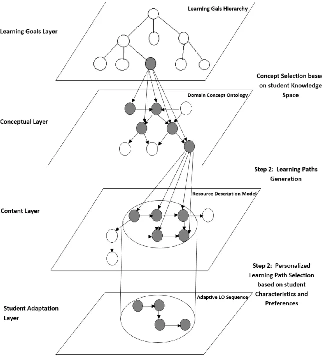
The Learning Path Graph represents and describes the structure of domain knowledge, learning goals, and all available learning paths as shown in Figure 2.2 [25, 26]. The Learning Path Graph, in e-learning systems has been modeled as a directed graph where each node represents a course unit and the directed edges describe the preceding relationship between the course units (nodes) [27]. The edge weight presents the difficulty level from one node to the next node [28]. Each node in the Learning Path Graph represents one or more concepts in order to build the Learning Path Graph and each concept of the Concept Path Graph associated with learning resources.

The Learning Path Graph can be used to determine the student’s movements between the course units according to the learning goals. An important concept that requires further research is how the optimal learning path arranges course units (nodes) according to student’s profile and needs [29].

(20)

9

Figure 2.2: Educational Hypermedia Sequence Layers and Personalized Learning Path Graph.

(21)

10

2.2.1.3 Course Learning Activity Technique

The Learning Activity Graph, as shown in Figure 2.3, is a directed graph with pre-conditions and post-pre-conditions in each node. The Learning Activity Graph is used to organize the learning resources according to a student’s learning activities [30].

The nodes of the graph can be a main learning activity or sub-learning activity. The graph contains several related learning resources for main learning activities and sub-learning activities. The Learning Activity Sequencing Algorithm integrates the use of a student’s model and Learning Activity Graph for Learning Activity Sequencing based on a student’s preference and level of expertise. This approach can generate efficient corresponding Learning Activity Sequences for various students by recording a student’s learning ability and achievements in order to update the student model.

Figure 2.3: Ontology-Based Learning Activity Sequencing in Personalized Education System.

(22)

11

2.2.1.4 Domain Ontology Technique

The related learning materials that generate the core course are grouped together and are described by the Domain Ontology to form a course. The Domain Ontology has the capability of providing adaptive e-learning environments and reusable educational resources.

Domain Ontology uses the class concept to represent the ontology through a set of abstract concepts, topics, and the semantic links between them. In this way, the knowledge of the treated domain is collected within the class concept [31].

Each class concept contains data type property and the class concept name. In order to identify the class concept and other object concept properties, a function is used to establish the different relationship between domain class concepts. The e-learning system compares the user’s learning style with various resource learning styles. Then, the proper learning materials that best fit the student’s individual request are developed.

2.2.2 Case Based Reasoning (CBR) and Genetic Algorithm

Technique

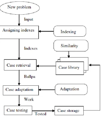
Case Based Reasoning as shown in Figure 2.4, adapts old solutions to meet new demands or interprets a new situation by reasoning from preceding situations [32]. The Case Based Reasoning planner is a learning system that has the ability to reuse its own experiences. Furthermore, through Case Based Reasoning, knowledge based learning makes the planner understands what should be learned and when it should be learned [32].

(23)

12

Figure 2.4: The reasoning procedure of CBR system.

In CBR, a new case occurs when the student fails to reach the mastery level in the current unit. This case triggers the CBR system to start a search for the case that is most comparable to the new case in order to support the corrective activity and predict the probabilities of that specific case. Within the CBR system, a Genetic algorithm is utilized. Here, the Genetic algorithm is based on different learning units and their difficult parameters for each unit in order to generate a learning path. The Genetic algorithm contains the following operations: the reproduction operations, the cross over operations, and the mutation operations. When this Genetic algorithm and the designed fitness function, within the Genetic algorithm based module, were applied to the course units, a personalized learning path was created [32].

(24)

13

2.2.3 Intelligence Techniques

These techniques use an artificial intelligence approach to generate an adaptive learning path.

2.2.3.1 Artificial Neural Network Technique

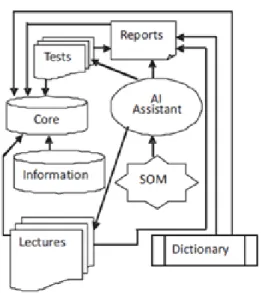
In order to generate an adaptive learning path by using this technique, an Artificial Intelligent Learning Assistant is applied. The Learning Assistant’s responsibility is to define the individual’s learning path for students in e-learning environments.

A Learning Assistant utilizes the two packages[33]. The first package trains the neural network by classifying every student into different student clusters based on their level of knowledge. The second package creates the learning path that is proper for the cluster into which the student has been classified.

Within the neural network exists the Self Organizing Map (SOM) shown in Figure 2.5, which is used for grouping similar students. SOM has two processes:

A. Training

In Training, the map is built by using input elements (examples). It is a competitive process also called vector quantization.

B. Mapping

In Mapping, SOM automatically classifies a new input vector, which means it classifies a new student into one of the student clusters. The learning path for this student is generated based on the learning path that is proper for the

(25)

14

cluster in which the student has been classified by the trained Self Organizing Map [33].

Figure 2.5: Interconnection between Pack agent in WebTeacher system.

2.2.3.2 Swarm Intelligence Technique

Swarm Intelligence is one of the techniques used in artificial intelligence. In this technique, the domain knowledge is classified as different learning units (objects). These objects include course level such as basic, itinerary, compulsory, and elective courses [34]. In addition, competencies with Swarm Intelligence are multidimensional, comprise of knowledge, skills, and psychological factors that are brought together in complex behavioral responses to environmental cues [35].

(26)

15

The Reusable Competency Definition (RCD) or competency records are used inside Swarm Intelligence in order to define the learning objects restrictions, prerequisites reflected from learning object metadata records, and the learning outcomes.

The Particle Swarm Optimization (PSO) Algorithm is an evolutionary computing optimization algorithm that determines the optimal learning path according to students’ needs.

2.2.4 Extended Ant Colony Technique

This technique combines the previous user’s learning and an Ant Colony system approach in order to generate an adaptive learning path [36].

The Ant Colony Optimization (ACO) technique predicts the best path based on the students’ profile and the previous learning paths that have been followed by the previous students.

The Extended Ant Colony technique is used in an Attribute based Ant Colony System (AACS) [36] which is an extension of the Ant Colony system. Its implementation is to locate the learning objects that would be suitable for student based on the most frequent learning paths followed by the previous students.

From different knowledge levels and different styles of students, the system updates the trails pheromones to create a powerful and dynamic learning object search mechanism [37].

In order to accomplish the learning object search mechanism, the following three prerequisites must be met:

(27)

16

C. The learning system has the student’s personal information that includes the student’s knowledge level and learning style;

D. Student’s personal information and learning units which have been provided by the teacher or the content designer; and

E. The learning system has a relationship that matchup between students and learning unit.

2.2.5 Bayesian Network Technique

The Bayesian probability theory also known as the Bayesian Network Technique uses statistical theories to generate adaptive learning paths [38]. The Bayesian Network Technique follows a two-step process to generate an adaptive learning path.

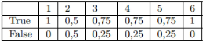
First, step 1 is based on Bayesian Probability Theory. In this approach, a node probability table is created as shown in Table2.1. This table has the node probability based on the candidate’s learning path, also referred to different consequent nodes, which could be traversed from the current node [38].

Table 2.1: Node Probability Table.

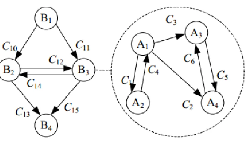
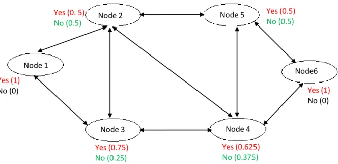
Then, in step 2 the Bayesian Network is created to calculate the probability value which represents each knowledge unit in the learning path as shown in Figure 2.6. To create

(28)

17

the candidate’s learning paths, the shortest path is selected to provide the appropriate learning path for students[38].

Figure 2.6: Bayesian network with probability value for each knowledge unit.

2.2.6 Adaptive Teaching Materials Generation Technique

The Adaptive Teaching Materials Generation Technique uses the Learning Path Algorithm to construct an adaptive course by personalizing the contents and teaching materials of the course [39]. This technique provides students with an adaptive learning environment based on the personalization of a student’s profile such as the level of their expertise, a student’s preference, and a student’s knowledge. The course content is dynamically adjusted during the learning and teaching process. This algorithm provides the ability to create online courses.

Node 2 Node 5 Node 1 Node 3 Node6 2 Node 4 Yes (0. 5) No (0.5) Yes (1) No (0) Yes (0.75) No (0.25) Yes (0.5) No (0.5) Yes (0.625) No (0.375) Yes (1) No (0)

(29)

18

Each user logs into the system specifying membership in a given user class. Then, the student searches for a specific topic, and consequently, all of the related learning paths are generated based on the student’s needs. The student chooses one of these paths and attends the course, which also includes exercises and tests.

2.2.7 Weighted Learning Object Technique

In this technique, three phases are implemented to generate an adaptive course [40]: Phase 1: Evaluate the learning process of the student;

Phase 2: For each student related to the student model; the student selects an appropriate course based on the weights of the learning object. The course’s materials such as text, images, and video are stored in the learning object database and some attributes for each learning object (difficulty level of learning object, total time needed for studying etc). Each attribute is assigned a value between 0 and 1 as a weight value of the learning object. Based on the student’s level of expertise, learning preferences, and student knowledge, the adaptive course contents are generated.

Phase 3: Select the view model of the course for each student.

2.2.8 Petri Nets Based Technique

To create an adaptive learning path through Petri Nets Based Technique, a two-step process is followed. The first step is to create a P-timed Petri Net based model for the hypertext learning state space. Then, the second step maps the learning state into places where a place receives tokens within the mapping learning state. Once this occurs, then the

(30)

19

knowledge node becomes accessible to students. The students are required to concentrate on their current learning state and freely select the knowledge node inside the current state. To describe the time function of the learning system, time can be associated with attributes: Places (called P-timed), Tokens (called age), and Transitions (called T-timed). In P-timed Petri nets, when an attribute is associated with Place, the firing rules will take a fixed and finite amount of time delay. Then, the system enables the transition for students. Within the learning environment, the learning activities consist of a series of discrete events, such as reading hypertext, typing words, and clicking hyperlinks. These activities help the students move through hyperspace [41, 42].

2.3 Summary

The current challenge in designing adaptive systems is to provide personalized courses to different students with different learning techniques closer to practical use and to be efficient [43, 44].

Many adaptive algorithms become available, based on these verities, adaptive algorithms have different capabilities in manipulating the learning systems and none of these algorithms are suitable for all tasks and situations.

The Learning Path Graph represents and describes the structure of domain knowledge, the learning goals and all available learning paths.

Based on the student’s learning paths and learning goals, the student’s attributes like the level of knowledge, learning style and preferences are used to select a personalize learning path from the Learning Path Graph. Concept Map represents the entire course

(31)

20

structure and the knowledge of the course domain. The role of Ontology is to describe the learning materials that are grouped together to form a course.

The students are grouped by using the clustering technique based on their learning styles. The technique using Bayesian Networks to generate adaptive learning path based on learning styles, level of expertise, etc.

Based on Bayesian Probability Theory, a node probability table is created. This table has the node probability based on candidate learning paths, which are the different consequent nodes and could be traversed from the current node. Then the Bayesian network is constructed to calculate the probability value, which represents each knowledge unit in the learning path. To create candidate learning paths, the shortest path is selected to provide the appropriate learning path for students.

This research focuses on optimal adaptive learning paths and students with different educational background, expertise, learning styles and learning preferences. Although all students will have the same learning goals, every student’s needs are adjusted in order to provide a suitable learning path to each individual and with suitable learning materials.

It is a complex task for teachers to design the learning material, the learning activities, and offer with different educational techniques tailored for individual students.

We need to emphasize on additional adaptation features, adaptive learning materials and smart techniques that can be used to identify the learning style, different educational experiences, skills, learning and learning preferences based on student’s interactions and different types of learning mode that lead to better learning abilities.

(32)

21

The aim of our research is to develop new adaptive algorithms tailored to individual needs. We will combine these new algorithms with a new adaptive system prototype, which provides students with all paths according to each student’s needs to satisfy the learning objectives.

(33)

22

res ea rch ers

CHAPTER 3: RESEARCH PLAN

3.1 Introduction

Adaptive e-learning researchers explore and develop adaptive techniques that provide a better educational experience for students. Researchers offer accurate and personalized content to students in an intelligent way [45], that may allow for adjustments in course content based on students most recent performance. This technique allows the student to skip unnecessary learning activities by providing automated and personalized support for the student [46]. Students with different educational backgrounds are the main challenge of the e-learning and m-learning systems. These systems provide personalized course units that meet the different students’ educational needs.

A directed graph represents an accurate picture of course descriptions for online courses through computer-based implementation of various educational systems [47]. E-learning and m-E-learning systems are modeled as a weighted directed graph where each node represents a course unit (CU). The Learning Path Graph represents and describes the structure of domain knowledge, including the learning goals, and all other available learning paths. This research proposes optimal adaptive learning path algorithms that use the student’s information from their profile in order to improve students’ learning

(34)

23

performance through e-learning and m-learning systems that provide suitable course content sequence in a dynamic form for each student.

3.2 Learning Path Graph

In general, the Learning Path Graph illustrates the structure of domain knowledge and the learning goals and all available learning paths.

In order to create and generate a Domain Concept Module, a two-step procedure is implemented.

The first part consists of designing Learning Goals Hierarchy and Concepts Hierarchy of the Domain Concept Module.

Concepts Path Graph is a directed acyclic graph which represents the structure of the Concept Domain Module which is generated from the connection between the Learning Goals Hierarchy and the Domain Concept.

The Learning Path Graph is a directed acyclic graph which represents all possible learning paths that match the targeted learning goal. In order to build the Learning Path Graph, within each concept of the Concept Path Graph, associated learning resources are selected from the media database. The media database describes the educational characteristics of the learning resources.

The second part of Domain Concept Module includes a personalized learning path. A personalized learning path is selected from the graph that contains all the available learning paths according to the characteristics of the student module. The student module

(35)

24

identifies a level of student expertise (student knowledge space), learning style (cognitive characteristics) and preferences. The suitability function is applied in order to find the weight of each connection of the learning path graph to provide a suitability factor for the learning resources.

By applying the shortest path algorithms to the weighted graph, the system will generate the optimal learning path for a specific student.

3.3 User Profile

The main challenge of the e-learning and m-learning systems is to create an appropriate adaptive course sequence to provide different students with different educational backgrounds.

One of the most important aspects of these systems which has not been thoroughly examined, is the capability of the learning system to adapt to the students’ profile. Optimal adaptive learning path algorithms use the student’s information from their profile to improve the e-learning and m-learning systems and to provide suitable course content sequence in a dynamic form for each student [48].

3.4 Graph Represents Course Units

Graphs are considered as an efficient representation of online courses and were used in the implementation of e-learning and m-learning systems. The course content is divided into portions called learning atoms that could be implemented at all levels and learning modes [48]. Each course unit could be represented as a graph that includes the

(36)

25

learning objectives located on the nodes and after the partition of the nodes. The graph will contain course concepts (Slide, Text, Examples, and Video) [49].

3.5 Learning Shortest Path

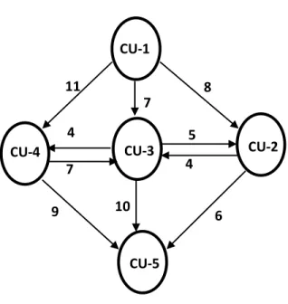
Figure 3.1, represents the course units that consist of n units whereas G is a graph with n vertices where N >= 0. Let V (G) = {v1, v2, …..,vn}. W is a two dimensional N x N

matrix such as:

W

(

i

,

j

)

=

{

𝑊𝑖𝑗 𝑖𝑓 (𝑣𝑖, 𝑣𝑗)𝑖𝑠 𝑎𝑛 𝑒𝑑𝑔𝑒 𝑖𝑛 𝐺 𝑎𝑛𝑑 𝑊𝑖𝑗 𝑖𝑠 𝑡ℎ𝑒 𝑤𝑒𝑖𝑔ℎ𝑡 𝑜𝑓 𝑒𝑑𝑔𝑒 (𝑣𝑖, 𝑣𝑗)

∞ 𝑖𝑓 𝑡ℎ𝑒𝑟𝑒 𝑖𝑠 𝑛𝑜 𝑒𝑑𝑔𝑒 𝑓𝑟𝑜𝑚 𝑣𝑖 𝑡𝑜 𝑣𝑗

Figure 3.1: Weighted graph represents course unit (CU) structure.

CU-3 CU-4 CU-2 CU-5 CU-1 6 11 8 9 7 4 5 10 4 7

(37)

26

The Adaptive Shortest Path consists of two stages: In stage 1, Algorithm 3.1 identifies the minimum cost matrix between each pair of course learning units. In stage 2, Algorithm 3.2 constructs an optimal learning path for each student. The Adaptive Shortest Learning Paths design an adaptive environment for individual students based on the minimum cost between each pair of the course learning units and their relevant personal information.

In stage 1, in order to locate the minimum cost matrix between each pair of the course learning units, we applied Algorithm 3.1. Algorithm 3.1 was implemented through the following steps:

(38)

27

Algorithm 3.1

Step 1: Input matrix W which represents the weighted graph course units’(CU) structure;

Step 2: For X = 1 to X < N repeat step 3 to step 7 where N is equal to number of CUs;

Step 3: For I = 1 and I <= N repeat step 4;

Step 4: For J = 2 and J <= N repeat step 5, step 6 and step 7;

Step 5: Compare If WIJ > (WIX + WXJ), if true then [50]

{

WIJ = (WIX + WXJ);

Compare If PIX = 0, if true then

PIJ = X+1;

Else PIJ = PIX;

}

Step 6: Compare If WIJ < (WIX + WXJ), if true then

No change;

Step 7: Compare If WIJ = (WIX + WXJ), if true then

{

WIJ = (WIX + WXJ);

Compare If PIX = 0, if true then

PIJ = X+1;

Else

PIJ = PIX;

}

Create new PcmID+1(I,J) = CU (Alternative path for IJ);

Create new W+1(I,J) = CU (Alternative minimum cost for IJ) where

(39)

28

Step 9: End

We assumed that there is no path between the same node, so for each I = J then WIJ

= ∞ and where each WIJ = ∞ then PIJ = ∞ was modified.

In stage 2; in order to identify the shortest path movement between each pair of the course learning units we, applied Algorithm 3.2.

Algorithm 3.2

Algorithm 3.2 represents the shortest path movement between CUI and CUJ. We

followed the steps listed below:

Step 1: CUI start node and CUJ end node (Target node);

Step 2: if PIJ = ∞ then no path between CUI and CUJ go to Step 7;

Step 3: If PIJ = 0, if true then

{

PIJ is end node (Target node in shortest path);

Go to Step 7;

}

Step 4: Repeat Step 5, Step 6 and Step 3;

Step 5: PIJ is next node in shortest path;

Step 6: I = PIJ;

(40)

29

3.6 Mathematical view

To explain how the algorithms work, first, we created an initial weighted matrix W=WIJ, where WIJ is the arrowhead weight from CUI to CUJ.

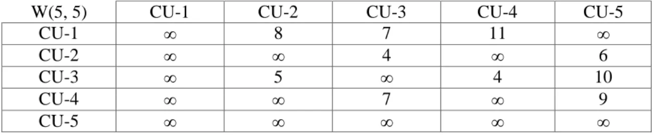
Then, we initialized the weighted matrix W from graph in Figure 3.1 as shown in Table 3.1 as follows:

 If no arrowhead exists between the two CUs, then the WIJ = ∞.

 For each I = J, then WIJ = ∞.

W(5, 5) CU-1 CU-2 CU-3 CU-4 CU-5

CU-1 ∞ 8 7 11 ∞

CU-2 ∞ ∞ 4 ∞ 6

CU-3 ∞ 5 ∞ 4 10

CU-4 ∞ ∞ 7 ∞ 9

CU-5 ∞ ∞ ∞ ∞ ∞

Table 3.1: Graph from Figure 3.1 represented by W(N,N) matrix, where N is the number of course units = 5.

Then, we created Table 3.2, where P is path matrix: P is a two dimensional N x N matrix such that for each P(I,J) = { p11 = p12 = p13 …. pnn = 0}:

P(5,5) CU-1 CU-2 CU-3 CU-4 CU-5

CU-1 0 0 0 0 0

CU-2 0 0 0 0 0

CU-3 0 0 0 0 0

CU-4 0 0 0 0 0

CU-5 0 0 0 0 0

(41)

30

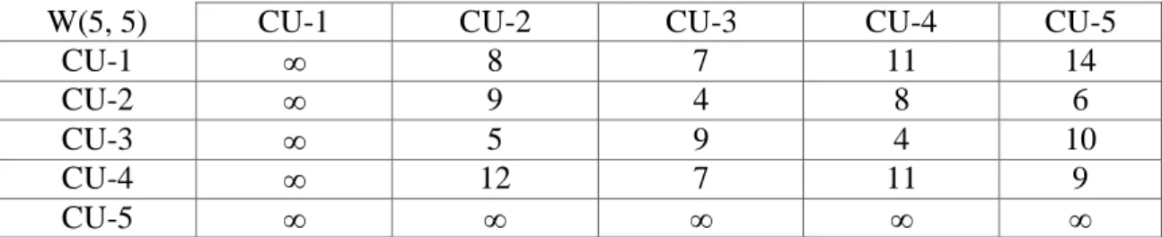
After applying Algorithm 3.1, in stage 1, we generated Table 3.3 and Table 3.4:

W(5, 5) CU-1 CU-2 CU-3 CU-4 CU-5

CU-1 ∞ 8 7 11 14

CU-2 ∞ 9 4 8 6

CU-3 ∞ 5 9 4 10

CU-4 ∞ 12 7 11 9

CU-5 ∞ ∞ ∞ ∞ ∞

Table 3.3: Shortest path traveling cost matrix W(I,J) between any CUs.

P(5,5) CU-1 CU-2 CU-3 CU-4 CU-5

CU-1 0 0 0 3 2

CU-2 0 3 0 3 0

CU-3 0 0 2 0 0

CU-4 0 3 0 3 0

CU-5 ∞ ∞ ∞ ∞ ∞

Table 3.4: Shortest path traveling matrix P(I,J) for CUs.

After applying to each I = J for cost matrix, then W(I,J) = ∞ as shown in Table 3.5: W(5,5) CU-1 CU-2 CU-3 CU-4 CU-5

CU-1 ∞ 8 7 11 14

CU-2 ∞ ∞ 4 8 6

CU-3 ∞ 5 ∞ 4 10

CU-4 ∞ 12 7 ∞ 9

CU-5 ∞ ∞ ∞ ∞ ∞

(42)

31

After applying to each, W(I,J) = ∞ then P(I,J) = ∞ as shown in Table 3.6: P(5,5) CU-1 CU-2 CU-3 CU-4 CU-5

CU-1 ∞ 0 0 3 2

CU-2 ∞ ∞ 0 3 0

CU-3 ∞ 0 ∞ 0 0

CU-4 ∞ 3 0 ∞ 0

CU-5 ∞ ∞ ∞ ∞ ∞

Table 3.6: Shortest path traveling matrix P(I,J) for each W(I,J) = ∞, then P(I,J) = ∞. In stage 2, Algorithm 3.2 was applied in order to find the shortest path movement between the learning CUs according to the results shown in Table 3.6.

Now we need to find the shortest path cost CU1CU5. The solution is reflected in Table 3.5 where W (1,5) = 14. Then, we determine the path movement between CU1 and CU5. In order to complete this task, we use Table 3.6 to locate the path movement between CU1 and CU5 as follows:

From Table 3.6 the path beginning with CU1CU5 = 2, then CU2CU5 = 0 (end nod), then the path is CU1CU2CU5.

3.7 Adaptation of the Learning Shortest Path Algorithms to the Relevant

Personal Student Information

In our first scenario, we assume the student is at the initial stage and logs into the system, and the student begins the coursework with the CU1. After the student successfully finishes and wants to continue onto CU2, the system will direct the student towards the shortest path CU1CU2 which is equal to 8.

(43)

32

In the second scenario, assume the student has completed the coursework in CU1 and CU2 and has logged out of the system. The student, then, decides to log back into the system to complete CU3, the system automatically directs the student from CU1CU3 which is equal to 7. The system does not take CU2 into consideration and ultimately affects the student learning path based on student’s personal information.

To make the Algorithm 3.2 more adaptive to the student’s profile, the flow of Algorithm 3.3 must be accordingly. Once the student completes a new CU, the system will update the student’s personal profile with the new information. Therefore, if the student decides to learn the new CU, the system will identify the shortest path between each CU in the student’s profile as well as any new CUs that the student plans to study.

Algorithm 3.3

Step 1: For each CU learned in the student’s profile complete Step 2;

Step 2: Find the shortest path between CUs in the student’s profile and new target CU by using the result from Table 3.5;

Step 3: Find the minimum cost from all of the shortest paths to the new target CU between CUs in the student’s profile and the new CU target;

Step 4: Then determine the shortest path according to the student’s profile that reflects the CUI (min cost) to the new target CU;

Step 5: Use Algorithm 3.2 and Table 3.6 to find the shortest path movement between learning CUI (min cost) and new target CU;

(44)

33

Step 6: If student complete the newly targeted CU, then the student’s personal profile

will automatically be updated by the system;

Step 7: End.

Once Algorithm 3.2 has been modified, then in following scenario assumes the student is at the initial stage and logs into the system, the student completes CU1. After CU1 is completed, the student moves onto CU2 and the system will direct the student to the shortest path CU1CU2 which is equal to 8. This information is stored in the student’s profile.

However, the next time the student logs onto the system to study CU3, by applying Algorithm 3.3 according to the student’s profile, the system will compare CU1CU3 = 7 with CU2CU3 = 4 and then, the system will direct the student to the path CU2CU3 which is equal to 4.

The personalization of a student’s learning path is the core feature of the e-learning and m-learning systems processes. Our current algorithms will be used to construct an adaptive m-learning prototype for Computer Science courses.

(45)

34

3.8 Automatic Detection of Learning Style

Figure 3.2: AML System Contents according to Learning Style.

Our AML system presents course instruction for students by using the shortest path algorithm in order to find the most efficient learning path between the learning course units (CUs), according to students’ profiles. In order to discover the most effective path, we need to implement and use learning style methods in the designing stage of course content.

(46)

35

According to a student’s learning style, we can introduce the same course content through different presentation methods as shown in Figure 3.2. In our AML system design, we used the Data Driven Method based on the Index of learning style questionnaires created by Felder and Soloman [51]. In addition, we used the Literature Based Method [52] that uses the students’ behavior in order to determine a student’s learning style. Both the Data Driven Method and the Literature Based Method were used as base tools for analyzing students’ learning styles.

The Index of Learning Styles is used for identifying learning style preferences in the Felder and Soloman model. The Index of Learning Styles has 44 questions. The Felder and Soloman model has four dimensions where each dimension defines two differing learning styles. Each dimension has 11 questions containing two options). Also, each dimension uses scaling values between -11 to +11.

The student’s results indicate which learning style the student like better, for example if a student’s scaling result is between -3 to +3, then the student prefer the two learning styles of the dimension equally. Otherwise, the student prefers one learning style more than the other of the dimension [53].

The reason for the Index of Learning Style questionnaire is that it provides us with important information to determine the type of content necessary for the students according to their learning styles. The Index of Learning Style questionnaire can be easily implemented to analyze the students’ learning styles [54].

(47)

36

According to the model introduced by Felder and Soloman and [55-57], the learning contents in our AML system are categorized as shown in Table 3.7.

Table 3.7: Four Dimensions of Learning Style.

Our AML system can select appropriate learning styles with attention to the behavior and appropriate needs of the student. The AML system adapts to the student’s learning style by implementing a learning style assessment and the Literature Based Method. Both were used in our AML system to identify the student’s learning style. According to the Student Learning Style Module, this process can be completed in the following ways:

A. Initial Learning Style Adaptation: If the student decides not to take the learning style assessment based on the Felder and Soloman Index of Learning Styles, by default, the students learning styles are categorized as active, sensing, sequential, and visual. The AML system will provide

(48)

37

students with the appropriate learning content according to the Initial Learning Style [58, 59].

B. Student Learning Style Adaptation: At the beginning of the course, the AML system provides the student with the learning style assessment. If the student decides to take the learning style assessment, then the AML system will analyze the learning style assessment results and provide students with the right learning content according to the student’s learning style [60]. C. Literature Based Method Adaptation: The Literature Based Method is used

in our AML system to automatically identify students learning styles based on the features of Learning Style Module that describe students’ behaviors. The features and the behavior patterns in our Learning Style Module refer to the Felder and Soloman model that have been used in our system’s design. In our system, we adapt the following behavior patterns:

1. Active Learning Style: Can be identified by the number of exercises that a student completed, the number of questions that a student answered, and the number of questions that a student fails to answer twice or more.

2. Reflective Learning Style: Can be identified by the number of reviewed learning materials, and the time spent on this learning material.

3. Sensing Learning Style: Can be identified by the number of correct answers about facts, the number of correct answers after

(49)

38

reviewing the examples, and the number of correct answers after seeing practical material.

4. Intuitive Learning Style: Can be identified by the number of correct answers given after a theoretical explanation, the number of correctly answers about concepts, the number of correct answers about creating new solutions.

5. Visual Learning Style: Can be identified by the number of correct answers given after seeing graphs, charts, images and video, and time spent watching videos.

6. Verbal Learning Style: Can be identified by the number of correct answers given after reading text, and the number of correct answers given after listening to audio.

7. Sequential Learning Style: Can be identified by the number of times the student prefers to the step by step problem solving, and the number of correct answers about details.

8. Global Learning Style: Can be identified by the number of times the student decides to solve a problem directly, the number of reviewed outlines, and the time spent on outlines.

According to [61], the behavior patterns as described above and the students’ information based on these behavior are used to obtain the hints in order to calculate the student’s learning style. Hints are described as (hdim, i), where hints are collected for every

(50)

39

After we determine the relevant features (patterns) of students’ behavior, based on Felder and Soloman learning style model, we need to use a threshold value to classify the occurrence of behavioral patterns. The threshold value identifies the presence of behavioral patterns and categorized them based on the hint of 0 to 3, where, 0 = no information about students’ learning style, 1 = low (e.g., reflective), 2 = moderate does not provide a specific hint, and 3 = high (e.g., active). To find the student’s learning style, we apply the following [61]:

1. Sum up all hints and divide them by the number of patterns that include available information (Pdim).

2. Use formula 1 to measure the individual learning style (lsdim).

3. Use formula 2 to find (nlsdim), by normalizing the measure result from formula 1 on a range from 0 to 1.

(1)

(2)

Where 1 indicates a strong positive preference and 0 indicates a strong negative preference for the respective learning style. If no pattern includes existing information, no information about the learning style can be found.

𝑙𝑠dim = ∑ ℎdim, 𝑖

𝑃dim

𝑖=1

𝑛𝑙𝑠dim =𝑙𝑠dim − 1

(51)

40

The AML system will update the Learning Style Module with new information. Once a Learning Style Module is updated, the AML system will deliver only the learning content that is suitable to the student’s learning style.

3.9 Adaptive M-Learning System Prototype

The main characteristic of our AML (Adaptive Mobile Learning) system is that it can predict the student’s optimal learning process based on the student’s relevant background information, prior knowledge, learning preferences and student’s learning style. Through the implantation of our algorithms, the AML system identifies a student’s optimal shortest learning path.

This AML system was designed using System Interface, an Adaptive Engine Module, a Student Profile Module, a Learning Style Module, a Course Content Module, a Student Assessment Module, a Domain Concepts Module, and a Learning Path Generation Module. Figure 3.3 illustrates our AML systems architecture.

(52)

41

Figure 3.3: Adaptive M-learning system architecture.

3.9.1 System interface (SI)

System Interface includes Admin Interface Module (AIM), Instructor Interface Module (IIM) and Student Interface Module (SIM).

3.9.1.1 Admin Interface Module (AIM)

The Admin Interface Module enables the system administrator to access the Course Content Module, Student Profile Module, Learning Style Module, Course Content Module, Student Assessment Module, and the Domain Concepts Module.

AIM provides the services for the system administrator to define access control rules, access privileges [62, 63], maintain student enrollments, user profiles, course schedules [63], student examination, create course concept units, course material and

(53)

42

archives. AIM, also, provides the services for the system administrator to monitor the learning progress [64, 65].

The system administrator can also perform a number of system maintenance operations through various modules. In the Student Profile Module, the system can create, edit and delete a student profile [65, 66]. The system administrator can create, edit, and delete course material. In Student Assessment Module, the administrator manages exams [67].

3.9.1.2 Instructor Interface Module (IIM)

The Instructor Interface Module allows instructors to manage and control course subject pages [68], create and modify course material, manage and control online learning activities, and monitor students’ performance based on all types of exams and grading.

Through the Instructor Interface Module an instructor controls the active period that a student can access each lesson’s or exam. This Module prevents students from advancing to new lesson contents. A student must finish any test or exercises related to the student current course content [69].

3.9.1.3 Student Interface Module (SIM)

The Student Interface Module presents the educational material to the student in the most effective way. Through the SIM, students enter their personal information that is then saved to their profile database. As a first time user, SIM prompts the student to take Pre-test. This Pre-test evaluates the student’s knowledge, and the results are stored in the student’s profile.

(54)

43

Then, the system prompts the Adaptive Engine Module to create and provide personalized learning paths, according to a Student’s Profile Module and Learning Style Module results.

Based on these results, the student has an option to enroll in the available course units or search for a specific unit.

3.9.2 Student Profile Module (SPM)

A Student Profile Module is the key resource for facilitating our AML system process that represents essential information about each student. The Student Profile Module quantifies the student’s relevant background information, prior knowledge, learning preferences, learning style linked to Learning Style Module and a student’s personal information. Each student has his own profile which enables the system to deliver a personalized course learning path with customized course materials, based on the student’s learning style [70].

3.9.3 Learning Style Module (LSM)

It is observable that different students have different preferences, needs, and different ways to learn [71]. According to these differences the learning style indicates how a student learns and likes to learn [72] or gives perception that individuals differ in regard with what type of instruction or study is the most effective for them [73].

Our Learning Style Module predicts the student’s behavior through the Felder and Silverman module created for engineering students to classify them according to where they fit on a number of scales belonging to the ways in which they receive and process

(55)

44

information, the dimensions of the learning styles in this module, such as namely perception, input, processing, and understanding [74, 75].

When students are registered in the system, their learning styles need to be tested. The student needs to answer a short assessment that is used to determine student’s preferred learning style [76]. This style indicates a preference for some media type over others. The assessment results are stored in the Learning Style Module, which will be used for the initial adaptation in our system.

3.9.4 Domain Concept Module (DCM)

The Domain Concept Module is divided into two interconnected sub models: 1) Concept sub-Module contains information about the domain and the course

structure. Our Domain Concept Module was built based on a weighted directed graph, where each node represents a course unit while arcs represented relationships between course units as introduced in Section 3.2.

2) The Media Resources Sub-Module traces media preference where each concept in the Concept sub-Module composite contains with different media types such as audio, video, text, and pdf. From this information, we provide students with the best media that represent the course units according the students’ learning styles [77].

(56)

45

3.9.5 Course Content Module (CCM)

The entire course unit’ materials are stored in databases contained in the Course Content Module. In this module, it is easy to extend the database by adding new topics to any course unit.

The idea behind the separation of the Domain Concept Module and Course Content Module is to make it possible to reuse a part of or all of the course unit materials if we need to use these materials to build a different course with similar related materials.

3.9.6 Learning Path Generation Module (LPGM)

The graph in the Domain Concept Module contains all the possible learning paths. The Learning Path Generation Module has all the available personalized learning paths generated from the Adaptive Engine Module according to the student’s profile and his learning style.

3.9.7 Student Assessment Module (SAM)

In our Adaptive Mobile Learning system prototype, the Student Assessment Module is used to adapt the needs and traits of the students [78]. According to student performance assessment, we can dynamically generate suitable learning content to fit the student needs.

An online assessment can be designed to begin with a Pre-test, which is an assessment of a student’s pre knowledge of each learning unit before taking the course. Based on the Pre-test results, the system only presents course units necessary to the student

(57)

46

based on the learning objectives of the course. Also, there is Post-test for each unit that the student must pass in order to receive credit for each unit.

3.9.8 Adaptive Engine Module (AEM)

The Adaptive Engine Module uses the algorithms that integrate information from the preceding modules in order to select an appropriate learning path to present the course to the students [79].

The process of adaptive modeling starts with selecting representative nodes by analyzing the student’s needs from the Student Profile Module, Learning Style Module, and Assessment Module [80].

The Adaptive Engine Module performs two tasks. The first task is to find all the personal learning paths using adaptive algorithms detailed in section 3.5 which incorporates the Student Profile Module and Assessment Module, in order for the student to select one of these provided paths and attend the optimal learning path to study his course. The second task retrieves the related teaching material according to a student’s learning style.

(58)

47

CHAPTER 4: EXPERIMENTS AND RESULTS

In order to verify the analytical research results, experimental results are introduced in this section. For this experiment, we have used the Network Security course CPEG 561. CPEG 561 is a graduate course offered as an elective course for Computer Science and Computer Engineering students.

4.1 Statistical Power Analysis

This work proposes that our AML system improves the student’s performance more than control system. This section summarizes the statistical power analysis performed with the aim to test of the alternative hypothesis.

Let Mxdenote the mean for the AML group and Mydenote the mean for the Control group. The statistical Hypotheses for this work are as follows:

Ho: Mx − My = 0 Ha: Mx − My > 0

The difference significance is determined by the used Level of Significance (α). Significance level: α = 0.05.

(59)

48

4.1.1 T-test

The Student's t-test is used to assesses whether the mean (average) of two groups are statistically different from each other.

4.1.1.1 Pre-test

The Pre-test was designed to ensure that both the Control group and the Experimental group had the equivalent computer knowledge required for taking the Network Security course. The examination questions of the Pre-test included 25 multiple choice questions and true-false questions covering the content of tested units of Network Security course.

 Question: What was the average Pre-test score for the two groups: AML

experimental group and Control group?

As shown in Table 4.1 and Figure 4.1, we have examined the Pre-test results of the AML experimental group (N=15) and the Control group (N=15). For the AML experimental group, the average score was 57.87. For Control group the average score was 67.20.

(60)

49

Pre-test scores

AML experimental group Control group

48.00 64.00 56.00 84.00 52.00 72.00 60.00 84.00 56.00 52.00 60.00 40.00 84.00 76.00 56.00 64.00 64.00 80.00 36.00 48.00 60.00 72.00 80.00 56.00 48.00 60.00 56.00 84.00 52.00 72.00 Mx = 57.87 My = 67.20

Table 4.1: AML experimental group and Control group Pre-test scores.

Figure 4.1: AML experimental group and Control group Pre-test comparison graph.

0 10 20 30 40 50 60 70 80 90 100

Pre-test Results Chart

AML group Control group

(61)

50

 Question: When comparing the Pre-test results of the two groups, was there a

significant difference in scores (either positive or negative)?

Figure 4.2: Pre-test confidence intervals and estimated difference.

AML group Control group

Mean 57.8667 67.20 Variance 141.4095 192.4571 Stand. Dev. 11.8916 13.8729 N 15 15 T -1.9783 degrees of freedom 28 critical value 2.048

Table 4.2: t-test results of the Pre-test.

AML experimental group

Control group

Mean = 57.867 ± 6.585

(62)

51

Table 4.2 and Figure 4.2 present the t-test results of the Pre-test for both groups. As shown in Table 4.2, the mean of the Pre-test was 57.8667 and the standard deviation was 11.8916 for the AML experimental group. Whereas, the mean was 67.20 and the standard deviation was 13.8729 for the Control group. The p-value result indicates that the two groups do not significantly differ from each other at p < 0.05. Clearly, it is evident that the two groups of students have statistically equivalent abilities in learning of the Network Security course.

4.1.1.2 Post-test

The Post-test was proposed to compare the learning achievements of two groups of students after taking the Network Security course. The Post-test contained three essays and 90 multiple choice/ true-false questions that covered all of the units of the Network Security course.

Question: What was the average Post-test student’s score for AML experimental group

and Control group?

We examined the Post-test of the AML experimental group (N=15) and the Control group (N=15). As shown in Table 4.3, the average score was 66.56 for the AML experimental group. The average score was 45.97 for Control group.

(63)

52

Post-test scores

AML experimental group Control group

74.76 44.54 61.47 47.98 77.92 52.40 85.35 42.78 55.10 47.40 65.98 37.72 57.11 65.38 70.47 44.37 67.27 42.82 69.13 41.33 50.12 55.58 63.91 43.90 74.44 71.84 71.45 49.96 53.89 1.56 Mx = 66.56 My = 45.97