Weijie Zhong
Submitted in partial fulfillment of the requirements for the degree of
Doctor of Philosophy
in the Graduate School of Arts and Sciences
COLUMBIA UNIVERSITY 2019
Weijie Zhong All rights reserved
Essays on information acquisition
Weijie ZhongThis dissertation studies information acquisition when the choice of information is fully flexible. Throughout the dissertation, I consider a theoretical framework where a decision maker (DM) acquires costly information (signal process) about the payoffs of different al-ternatives before making a choice. In Chapter 1., I solve a general model where the DM
pays a cost that depends on the rate of uncertainty reduction and discounts delayed pay-offs. The main finding is that the optimal signal process resembles a Poisson signal — the signal arrives occasionally according to a Poisson process, and it drives the inferred posterior belief to jump discretely. The optimal signal is chosen to confirm the DM’s prior belief of the most promising state. Once seeing the signal, the decision maker is discretely surer about the state and stops learning immediately. When the signal is oth-erwise absent, the decision maker becomes gradually less sure about the state, and con-tinues learning by seeking more precise but less frequently arriving signals. In Chapter 2.,
I study the sequential implementation of a target information structure. I characterize the set of decision time distributions induced by all signal processes that satisfy a per-period learning capacity constraint on the rate of uncertainty reduction. I find that all decision time distributions have the same mean, and the maximal and minimal elements by mean-preserving spread order are exponential distribution and deterministic distri-bution. The result implies that when the time preference is risk loving (e.g. standard or hyperbolic discounting), Poisson signal is optimal since it induces the riskiest exponential decision time distribution. When time preference is risk neutral (e.g. constant delay cost), all signal processes are equally optimal. In Chapter 3., I relax the assumption on
ported by sequential minimization iff it satisfies: 1) monotonicity in Blackwell order, 2) sub-additivity in compound experiments and 3) linearity in mixing with no information. Then I study a dynamic information acquisition problem where the cost of information depends on an indirect information measure and the delay cost is fixed (the DM is time-risk neutral). The optimal strategy is to acquire Poisson type signals. The result implies that when the cost of information is measured by an indirect measure, Poisson signals are intrinsically cheaper than other signal processes. Chapter 4.introduces a set of useful
technical results on constrained information design that is used to derive the main results in the first three chapters.
List of Figures. v
Acknowledgments. viii
Dedication. x
Introduction. 1
1 Optimal dynamic information acquisition. 6
1.1 Introduction. . . 7
1.2 Related literature. . . 13
1.2.1 Dynamic information acquisition. . . 13
1.2.2 Rational inattention. . . 14
1.2.3 Information design. . . 16
1.2.4 Stochastic control. . . 16
1.3 Model setup. . . 17
1.3.1 Motivation for a flexible model. . . 23
1.4 Dynamic programming and HJB equation. . . 24
1.5 The auxiliary discrete-time problem. . . 28
1.5.1 Discrete-time problem. . . 28
1.5.2 Discrete-time Bellman equation. . . 30
1.5.3 Convergence and verification theorem. . . 31
1.6 Optimal information acquisition. . . 32
1.6.1 Main characterization theorem. . . 33
1.7.1 Linear delay cost. . . 51
1.7.2 General information measure. . . 53
1.7.3 Linear flow cost. . . 57
1.8 Applications. . . 59
1.8.1 Choice accuracy and response time. . . 59
1.8.2 Radical innovation. . . 62
1.9 Conclusion. . . 65
2 Time preference and information acquisition. 66 2.1 Introduction. . . 67
2.2 Setup of model. . . 75
2.3 Solution. . . 77
2.3.1 An auxiliary problem. . . 77
2.3.2 Optimal learning dynamics. . . 78
2.3.3 Gradual learning v.s. decisive evidence. . . 80
2.4 Continuous time model. . . 82
2.4.1 Implementation. . . 84
2.5 Discussion. . . 86
2.5.1 Optimal target signal structure. . . 86
2.6 Conclusion. . . 88
3 Indirect information measure and dynamic learning. 89 3.1 Introduction. . . 90
3.2 Indirect information measure. . . 93
3.2.1 Information structure and the measure of informativeness. . . 93
3.3.1 Model. . . 100
3.3.2 Solution. . . 103
3.3.3 Existence and uniqueness. . . 108
3.4 Conclusion. . . 110
4 Information design possibility set. 111 4.1 Introduction. . . 112
4.2 Information possibility set. . . 113
4.3 Main theorem. . . 118
4.3.1 Existence and finite support. . . 118
4.3.2 Necessary condition for the maximizer. . . 119
4.3.3 Convex optimization. . . 120
4.3.4 Maximum theorem. . . 122
4.4 Applications. . . 123
4.4.1 Costly Information acquisition. . . 123
4.4.2 Dynamic information design. . . 124
4.4.3 Persuade voters with outside options. . . 126
4.4.4 Screening with information. . . 128
4.5 Conclusion. . . 130
4.6 Theorems used in proof. . . 130
References. 131 A Appendix for Chapter 1. 138 A.1 Further discussions. . . 139
A.1.3 General state space. . . 143
A.1.4 Discrete-time information acquisition. . . 146
A.2 Omitted proofs. . . 150
A.2.1 Roadmap for proofs. . . 150
A.2.2 Proof of Theorem 1.1. . . 151
A.2.3 Proof of Theorem 1.2. . . 167
B Supplemental materials for Chapter 1. 184 B.1 Proofs in Section 1.5.. . . 185
B.1.1 Useful lemmas. . . 185
B.1.2 Proof of Lemma 1.2. . . 201
B.1.3 Convergence. . . 208
B.2 Proofs in Section 1.6. . . 219
B.2.1 Proof and lemmas of Theorem 1.2. . . 219
B.2.2 Proof of Theorem 1.3. . . 239
B.3 Proofs in Section 1.7.. . . 265
B.3.1 Linear delay cost. . . 265
B.3.2 General information measure. . . 266
B.3.3 Linear cost function. . . 271
B.4 Proofs in Section 1.8.. . . 276
B.4.1 Choice accuracy and response time: proof of Proposition 1.1. . . 276
B.4.2 Radical innovation: proof of Propositions 1.2 and 1.3. . . 278
B.5 Proofs in Appendix A.1.. . . 282
B.5.1 Convergence of policy. . . 282
B.5.4 Axiom for posterior separability. . . 304
C Appendix for Chapter 2. 305 C.1 Omitted proofs. . . 306 C.1.1 Proof of Lemma 2.1. . . 306 C.1.2 Proof of Theorem 2.1. . . 308 C.1.3 Proof of Lemma 2.2. . . 312 C.1.4 Proof of Lemma 2.3. . . 313 C.1.5 proof of Theorem 2.3. . . 314 C.1.6 Proof of Lemma 2.4. . . 318
D Appendix for Chapter 3. 319 D.1 Proof in Section 1.3. . . 320 D.1.1 Proof of Proposition 3.2. . . 320 D.2 Proof in Section 3.3. . . 323 D.2.1 Proof of Theorem 3.1. . . 323 D.2.2 Proof of Proposition 3.3. . . 335 D.2.3 Proof of Proposition 3.5. . . 339
1.1 Incremental information. . . 21
1.2 Breakthroughs. . . 21
1.3 Partially revealing evidence. . . 22
1.4 Comparison. . . 22
1.5 Value and policy functions. . . 37
1.6 Dynamics of optimal policy. . . 38
1.7 Example with four alternatives. . . 38
1.8 Example with one-sided search. . . 39
1.9 Concavification of the gross value function. . . 41
1.10 Precision-frequency trade-off. . . 44
1.11 Confirmatory v.s. contradictory. . . 46
1.12 Continuing vs. stopping. . . 47
1.13 LP and QP plots. . . 60
1.14 The critical beliefs of different difficulty levels. . . 61
1.15 Value function. . . 64
1.16 Policy function.. . . 64
2.1 Belief trajectory. . . 68
2.2 Belief distribution of Gaussian learning. . . 71
2.3 Belief distribution of Poisson learning. . . 72
2.4 PDFs. . . 72
2.5 Integral of CDFs. . . 72
A.1 Convergence of policy function. . . 141
A.4 Policy function with 3 states. . . 146
A.5 Roadmap for proofs.. . . 150
A.6 Construction of optimal value function.. . . 168
B.1 Phase diagram ofpµ9,ν9q.. . . 226
I would like to thank my dissertation committee members, Yeon-Koo Che, Navin Kar-tik, Qingmin Liu, Andrea Prat and Mark Dean. First of all, I would like to express my deepest gratitude to my principle advisor Yeon-Koo Che for his constant guidance and support, and for serving as my role model of a truly insightful, rigorous and diligent economist. I am indebted to my advisor Navin Kartik for his invaluable directions and comments throughout my research. He expanded my intellectual curiosity and academic interest in economic theory. I am extremely grateful to Qingmin Liu, who exerted tremen-dous effort to help me build up my skills and shape my taste for research. I am also grate-ful to Andrea Prat, for delivering an inspiring economic theory course which attracted me to explore the field, and for his excellent feedbacks at all stages of my works. I would also like to thank Mark Dean who provided insightful feedbacks to my work and deepened my understanding of economic theory.
It was my great pleasure collaborating with my coauthors Teddy Kim, Konrad Mieren-dorff and Xianwen Shi, together with Yeon-Koo Che, Navin Kartik and Qingmin Liu. I sincerely thank them not only for contributing significantly to the projects, but also for tolerating my ignorance and sluggish, and turning me into a better scholar.
The entire theory group at Columbia university has unanimously supported me through-out my doctoral study. In particular, I want to thank Marina Halac and Pietro Ortoleva for discussing the contents of this dissertation with me for numerous times and for giving all kinds of useful advice beyond just research. I received very useful feedbacks on my research and advices for my career from Xiaosheng Mu, Jacopo Perego and Evan Sadler, to whom I am also extremely grateful.
For helpful comments and discussions on this dissertation, I am also grateful to Syl-vain Chassang, Johannes Hörner, Jakub Steiner, Philipp Strack, Tomasz Strzalecki,
An-University. In particular, Benjamin Golub, Yingni Guo, Shaowei Ke, Jonathan Libgober, Heng Liu, Harry Di Pei, Daniel Rappoport, Xingye Wu, Ming Yang and Jidong Zhou helped me a lot both in my research as scholars and on a personal level as friends.
On a personal level, I want to thank my schoolmates and friends for being encourag-ing and supportive regardless of my bad personality: Narisu Bai, Dawei Dencourag-ing, Jiayin Hu, Ang Li, Xuan Li, RC Xizhi Lim, Yifeng Liu, Yifeng Luo, Bo Qin, Qiuying Qu, Shuaiwen Wang, Peifan Wu, Danyan Zha, Qing Zhang, Yi Zhu. Finally, I would like to thank my parents and other friends. It is impossible to finish this dissertation without their support.
I dedicate the dissertation to my girlfriend Mengting Gu, who has provided me unconditional love and support, who hedged my risks when I chose to pursuit a risky career,
who guided me in making the most difficult decisions, and who induced a positive Poisson jump in my life.
This dissertation considers the following question: what is the optimal way to acquire information over time to learn about the payoffs of different options? This is a very clas-sic question that has been extensively studied in the literature starting from Wald (1947.)
and Arrow, Blackwell, and Girshick (1949.). However, we still do not have a complete
answer to this question, as the conventional approaches have been searching within very limited types of information, e.g. many models consider only Brownian motion type in-formation. Typically, papers in the literature study the optimal choice of “when to stop learning” taken a specific process of information as given, or the optimal control of a specific parameter of a given parametric family of information processes.
The goal of this dissertation is to answer the question by searching among all con-ceivable types of information, and completely endogenize the information acquisition strategy.
The practical motivation for permitting such flexibility in the type of information is that in practice the process of information acquisition can often be controlled in multi-ple aspects. The rapid development in statistics, data science and computer science is making information acquisition increasingly more flexible. For example, nowadays if a tech company wants to figure out the market’s response to an internal innovation, it can launch an A-B test on an online marketing platform, fine-tune hundreds of parameters of the test design and change them adaptively when data arrives. Another example is that FDA recently published its guidance ofadaptive design for clinical trials (see FDA (2018.)).
The guidance states that clinical trial designs with adaptive sample size, adaptive dose selection and response-adaptive randomization might improve the efficiency of the trials. In these examples, there is no a priori reason why some ad hoc restrictions on the type of information, e.g. the acquired data is generated from a normal distribution, are satisfied.
which can only be fully covered in a completely flexible information acquisition model. The theoretical framework for the entire dissertation is a sequential decision making model building upon the Wald framework. I consider a decision maker who makes a one-time choice from a set of actions, whose payoffs depend on a state unknown to the decision maker. The state is initially selected by the nature and remains fixed over time. At any instant of time, the decision maker chooses whether tostoplearning and select an action or continuelearning by choosingnonparametricallyan informative signal structure for the next moment of time. Both delaying the decision and acquiring information are costly. Of course, hardly any prediction can be made in a model with such generality. I will proceed by solving this optimization problem, keeping the full generality in the decision problem and information acquisition, but imposing three different sets of more restrictive assumptions on the cost of delay and the cost of information in the following three chapters.
In Chapter 1., entitled “Optimal dynamic information acquisition”, I study the case that
(i) the decision maker discounts delayed utilities in a standard way, (ii) the cost of in-formation depends on how fast the uncertainty about the unknown state is decreasing (also known as posterior separability). The goal of Chapter 1.is to fully solve for the
op-timal dynamic information acquisition strategy in a fairly general model with standard assumptions (discounting and posterior separable cost structure).
There are two main results. The first result states that although the model is non-parametric and allows fully flexible strategies, the optimal information acquisition strat-egy modeled as the induced posterior belief process can be restricted to a simple jump-diffusion processwithout loss. The second result fully characterizes the optimal belief pro-cess, which involves only a compensated Poisson jump process almost surely. In other words, it is optimal to conduct experiments that generate skewed and fat-tailed data.
is rare but a pass is a conclusive proof that the state is very likely and a corresponding action should be adopted immediately. Otherwise, failing the test does not immediately end the test. I also show that conditional on failures, the future tests have higher difficulty — passing rate is lower but a pass is more precise.
The analysis in Chapter 1. illustrates that the optimality of Poisson type signal
pro-cesses is a joint implication of the two assumptions in the model: exponential discount-ing and the information cost structure. Discussion in Appendix A.1.4.1.suggests that the
posterior separability assumptions is essentially a neutralitycondition: learning a target information structure through all equally costly strategies takes the same amount of time on average. To further understand the roll played by the two assumptions, I generalize each of them in the following two chapters.
In Chapter 2.on “Time preference and information acquisition”, I keep the assumption on
information cost and generalize the cost of delay to general convex or concave time cost. To get tractability in the model with further generality, I impose additional restrictions that (i) the flow cost of information acquisition is fixed (ii) the target decision rule is fixed. These restrictions shut down the dynamics of target decision rule and flow cost level, and highlight the implication of information on decision time. The main result of Chapter 2.
is that for all convex time cost functions, the optimal dynamic information acquisition strategy is aPoisson signal processthat either implements the target decision rule at a Pois-son rate or generates no information with large probability. For any concave time cost, the optimal dynamic information acquisition strategy is apure accumulationstrategy that only accumulates information but makes no decision until a deterministic date. Noticing that the neutrality condition makes all information acquisition strategy equally efficient on average. So the key implication of difference strategies is that the Poisson signal pro-cess induces decision in a riskiestway on the dimension of time: decision is either taken
minimizes time-risk involved in decision making.
Chapter 2.reveals a key implication of information acquisition: it determines the risk
in the decision making time. Therefore, under the neutrality condition (posterior separa-bility assumption), all information acquisition strategies induce the same expected deci-sion time and they only differ in the risks. Then, the preference on information acquisition strategies is solely pin down by the preference on time risk.
To deepen our understanding about the cost of information, I generalize the assump-tion on informaassump-tion cost in Chapter 3. on “indirect information measure and dynamic
learn-ing”. I assume that (i) the cost of delay is linear in time (time-risk neutral) and (ii) the cost of information depends on an indirect information measure. An indirect information measure takes an arbitrary cost function of information as primitive, and for each signal structure derives the minimized expected total cost from a sequence of signal structures that replicates the original signal structure. In other words, the assumption I put on the cost of information is essentially that (i) I allow within period sequential minimization of information measure, (ii) there is increasing marginal cost to the information measure per period. The main result of Chapter 3. is that the optimal signal process is a direct
compound Poisson signal: signal arrives according to a Poisson counting process and the arrival of signal suggests the optimal action directly, where the optimal action profile can be solved in an equivalent static rational inattention problem.
The analysis in Chapter 3. suggests that Poisson type information acquisition is not
only the “riskiest” when we restrict the information cost to satisfy neutrality i.e. all learn-ing strategies to be equally fast, it is also the “fastest” when we relax such restrictions on information cost, as long as the cost can be justified by within period information measure minimization.
de-ize the set of all combinations of expected value of finite objective functions from design-ing information. I show that the set is compact, convex and can be implemented by signal structures with finite support when the state space is finite. Moreover, the set as a corre-spondence of prior belief is continuous. Based on this result, I develop a concavification method of Lagrangian that works with general constrained optimization. Other appli-cations of the results include persuasion of receivers with outside options and screening using information.
1.1
Introduction
When individuals make decisions, they often have imperfect information about the payoffs of different alternatives. Therefore, the decision maker (DM) would like to ac-quire information to learn about the payoffs prior to making a decision. For example, when comparing new technologies, a firm may not know the profitability of alternative technologies. The firm often spends a considerable amount of money and time on R&D to identify the best technology to adopt. One practically important feature of the infor-mation acquisition process is that the choice of “what to learn” often involves considering a rich set of salient aspects. In the previous example, when designing the R&D process, a firm may choose which technology to test, how much data to collect and analyze, how in-tensive the testing should be, etc. Other examples include investors designing algorithms to learn about the returns of different assets, scientists conducting research to investigate the validity of different hypotheses, etc.
To capture such richness, in this chapter, I consider a DM who can choose “what to learn” in terms ofallpossible aspects, as well as “when to stop learning”. The main goal is to obtain insight into dynamic information acquisition without restriction on what type of information can be acquired. In contrast to my approach, the classic approach is to focus on one aspect while leaving all other aspects exogenously fixed. The seminal works by Wald (1947.) and Arrow, Blackwell, and Girshick (1949.) study the choice of “when to stop”
in a stopping problem with all aspects of the learning process being exogenous. Building upon the Wald framework, Moscarini and Smith (2001.) endogenize one aspect of
learn-ing, theprecision, by allowing the DM to control a precision parameter of a Gaussian signal process. Che and Mierendorff (2016.) endogenize another aspect of learning, thedirection,
by allowing the DM to allocate limited attention to different news sources, each biased in a different direction. Here, by allowing all learning aspects to be endogenous, the current
chapter contributes by studying which learning aspect(s) is(are) endogenously relevant for the DM and how the optimal strategy is characterized in terms of these aspects.
In the model, the DM is to choose from a set of actions, whose payoffs depend on a state unknown to the DM. The state is initially selected by nature and remains fixed over time. At any instant of time, the DM chooses whether to stop learning and select an action or to continue learning bynonparametricallychoosing the evolution of the belief process. The choice of a nonparametric belief process models the choice of a dynamic information acquisition strategy with no restriction on any aspect. I introduce two main economic assumptions. (i) The DM discounts delayed payoffs. (ii) Learning incurs a flow cost, which depends convexly on how fast the uncertainty about the unknown state is decreasing. The main model is formulated as a stochastic control-stopping problem in continuous time.
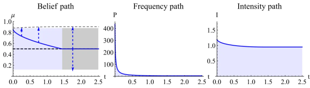
The main resultshows that the optimal strategy is contained in a simple family char-acterized by a few endogenously relevant aspects (Theorem 1.1.) and fully solves for the
optimal strategy in these aspects (Theorems 1.2.and 1.3.). Specifically, the first result states
that although the model is nonparametric and allows for fully flexible strategies, the belief process can be restricted to a simplejump-diffusion processwithout loss. In other words, a combination of aPoisson signal—a rare and substantial breakthrough that causes a jump in belief—and aGaussian signal—frequent and coarse evidence that drives belief diffusion— is endogenously optimal. A jump-diffusion belief process is characterized by four param-eters: thedirection,sizeandarrival rateof the jump, and the flow variance of the diffusion. The four parameters represent four key aspects of learning: the direction, precision and frequencyof the Poisson signal, and the precision of the Gaussian signal. The first result suggests that the DM need consider only the trade-offs among these aspects; any other aspect is irrelevant for information acquisition.
find that the Poisson signal strictly dominates the Gaussian signal almost surely, i.e. no resources should ever be invested in acquiring the Gaussian signal. The optimal Poisson signal satisfies the following qualitative properties in terms of the three aspects and the stopping time:
• Direction: The optimal direction of learning is confirmatory– the arrival of a Poisson signal induces the belief to jump toward the state that the DM currently finds to be most likely. As an implication of Bayes rule, the absence of a signal causes the belief to drift gradually towards the opposite direction, namely, the DM gradually becomes less certain about the state.
• Precision: The optimal signal precision isnegatively related to the continuation value. Therefore, when the DM is less certain about the state, the corresponding continuation value is lower, which leads the DM to seek a more precise Poisson signal.
• Frequency: The optimal signal frequency ispositively relatedto the continuation value. In contrast to precision, the optimal signal frequency decreases when the DM is less certain.
• Stopping time: The optimal time to stop learning is immediately after the arrival of the Poisson signal. Therefore, the breakthrough happens only once at the optimum. Then, the DM stops learning and chooses an optimal action based on the acquired information.
The optimal strategy is very heuristic and easy to implement. In the previous example, the firm can choose the technology to test, as well as the test precision and frequency. As a result, the optimal strategy is implementable. The optimal R&D process involves test-ing the most promistest-ing technology. The optimal test is designed to be difficult to pass, so good news comes infrequently, as in a Poisson process. A successful test confirms
the firm’s prior conjecture that the technology is indeed good and the firm immediately adopts the technology. Otherwise, the firm continues the R&D process. No good news is bad news, so the firm becomes more pessimistic about the technology and revises the choice of the most promising technology accordingly. The future tests involve higher passing thresholds and lower testing frequency. As illustrated by the example, although this chapter studies a benchmark with fully flexible information acquisition, the optimal strategy applies to more general settings where information acquisition isnotfully flexi-ble, but involves these salient aspects.
The main intuitionbehind the optimal strategy is a novelprecision-frequency trade-off. Consider a thought experiment of choosing an optimal Poisson signal with fixed direc-tion and cost level. The remaining two parameters—precision and frequency—are pinned down by the marginal rate of substitution between them. Importantly, the traoff de-pends on the continuation value. Due to discounting, when the continuation value is higher, the DM loses more from delaying the decision. Therefore, the DM finds it op-timal to acquire a signal more frequently at the cost of lowering the precision to avoid costly delay. In other words, the marginal rate of substitution of frequency for precision is increasing in the continuation value. As a result, frequency (precision) is positively (negatively) related to the continuation value.
In addition to precision and frequency, this intuition also explains other aspects. First, the Gaussian signal is equivalent to a special Poisson signal with close to zero precision and infinite frequency. The previous intuition implies that infinite frequency is generally suboptimal except when the continuation value is so high that the DM would like to sac-rifice almost all signal precision. As a result, the Gaussian signal is strictly suboptimal except for the non-generic stopping boundaries. Second, for any fixed learning direction, Bayes rule implies that the absence of a signal pushes belief away from the target direc-tion; to ensure the same level of decision quality the signal precision should increase over
time to offset the belief change. By acquiring a confirmatory signal, the DM becomes more pessimistic and, consequently, more patient over time. Therefore she can reconcile both incentives through reducing the signal frequency and increasing the signal precision. By contrast, if the DM acquires a contradictory signal, she becomes more impatient over time and prefers the frequency to be increasing. The two incentives become incongruent, thus, learning in a confirmatory way is optimal.
This intuition suggests that the crucial assumption for the optimal strategy is dis-counting — disdis-counting drives the key precision-frequency trade-off. This observation highlights the deep connection between dynamic information acquisition and the DM’s attitude toward time-risk. Discounting implies that the DM is risk loving toward payoffs with uncertain resolution time, as the exponential discounting function is convex. Intu-itively, the riskiest information acquisition strategy is a “greedy strategy” that front-loads the probability of success as much as possible, at the cost of a high probability of long delays. The confirmatory Poisson learning strategy in this chapter exactly resembles a greedy strategy. The key property of the strategy is that all resources are used in verify-ing the conjectured state directly and no intermediate step occurs before a breakthrough. By contrast, alternative strategies, such as Gaussian learning and contradictory Poisson learning, involve accumulating substantial intermediate evidence to conclude a success. The intermediate evidence in fact hedges the time risk: the DM sacrifices the possibility of immediate success to accelerate future learning.
Extensionsof the main model further illustrate the role played by each key assump-tion. The first extension replaces discounting with a fixed flow delay cost. In this spe-cial case, all dynamic learning strategies are equally optimal, as the cruspe-cial precision-frequency trade-off becomes value independent. This extension also illustrates that all learning strategies in the model are equally “fast” on average and differ only in “riski-ness”. This result further illustrates that the preference for time risk pins down the
opti-mal strategy. Second, I consider general cost structures and find that the (strict) optiopti-mality of a Poisson signal over a Gaussian signal is surprisingly robust: it requires a minimal con-tinuityassumption. Third, I study an extension where the flow cost depends linearly on the uncertain reduction speed. In this special case, learning has a constant return to signal frequency. As a result, the optimal strategy is to learn infinitely fast, that is, acquire all information at period zero.
This chapter provides rich implications by allowing learning to be flexible in all as-pects. First, the main results highlight the optimality of the Poisson signal compared to the widely adopted diffusion models. Specifically, the diffusion models are shown to be justified only under the lack of discounting. Second, the characterization of the optimal strategy unifies and clarifies insights from some existing results. In these results, although the DM is limited in her learning strategy, she actually implements the flexible optimum whenever feasible and approximates the flexible optimum when infeasible. Moscarini and Smith (2001.)’s insight that the “intensity” of experimentation increases in
continu-ation value carries over to my analysis. I further unpack the design of experiment and show that higher “intensity” contributes to faster signal arrival but lower signal precision. Che and Mierendorff (2016.) make same prediction about the learning direction as that of
my analysis when the DM is uncertain about the state. But they predict the opposite when the DM is more certain about the state– the DM looks for a signal contradicting the prior belief. I clarify that the contradictory signal is an approximation of a high-frequency confirmatory signal when the DM is constrained in increasing the signal frequency.
The rest of this chapter is structured as follows. The related literature is reviewed in Section 1.2.. The main continuous-time model and illustrative examples are introduced
in Section 1.3.. The dynamic programming principle and the corresponding
Hamilton-Jacobi-Bellman (HJB) equation are introduced in Section 1.4.. I analyze an auxiliary
the optimal strategy and illustrates the intuition behind the result. In Section 1.7.I discuss
the key assumptions used in the model. Section 1.8.explores the implications of the main
model on response time in stochastic choice and on a firm’s innovation. Further discus-sions of other assumptions are presented in Appendix A.1., and key proofs are provided
in Appendix A.2.. All the remaining proofs are relegated to Appendix B..
1.2
Related literature
1.2.1 Dynamic information acquisition
This chapter is closely related to the literature about acquiring information in a dy-namic way to facilitate decision making. The earliest works focus on the duration of learning. Wald (1947.) and Arrow, Blackwell, and Girshick (1949.) analyze astopping
prob-lemwhere the DM controls the decision time and action choice given exogenous informa-tion. Moscarini and Smith (2001.) extend the Wald model by allowing the DM to control
the precision of a Gaussian signal. A similar Gaussian learning framework is used as the learning-theoretic foundation for the drift-diffusion model (DDM) by Fudenberg, Strack, and Strzalecki (2018.). Following a different route, Che and Mierendorff (2016.), Mayskaya
(2016.) and Liang, Mu, and Syrgkanis (2017.) study the sequential choice of information
sources, each of which is prescribed exogenously.
Other frameworks of dynamic information acquisition include sequential search mod-els (Weitzman (1979.), Callander (2011.), Klabjan, Olszewski, and Wolinsky (2014.), Ke and
Villas-Boas (2016.) and Doval (2018.)) and multi-arm bandit models (Gittins (1974.), Weber
et al. (1992.), Bergemann and Välimäki (1996.) and Bolton and Harris (1999.)). These
frame-works are quite different from my information acquisition model. However, the forms of information in these models are also exogenously prescribed, and the DM has control over only whether to reveal each option.
the DM can design the information generating process nonparametrically. In a similar vein to this chapter, two concurrent papers Steiner, Stewart, and Matˇejka (2017.) and
Hébert and Woodford (2016.) model dynamic information acquisition nonparametrically;
however they focus on other implications of learning by abstracting from sequentially smoothing learning. In Steiner, Stewart, and Matˇejka (2017.) the linear flow cost
assump-tion makes it optimal to learn instantaneously, whereas in Hébert and Woodford (2016.),
the no-discounting assumption makes all dynamic learning strategies essentially equiva-lent.1. By contrast, the main focus of this chapter is on characterizing the optimal way to
smooth learning. I analyze the setups of these two papers as special cases in Sections 1.7.1.
and 1.7.3..
A main result of this chapter is the endogenous optimality of Poisson signals. Sec-tion 1.7.2.shows a more general result: a Poisson signal dominates a Gaussian signal for
generic cost functions that are continuous in the signal structure. This result justifies Pois-son learning models, which are used in a wide range of problems, e.g., Keller, Rady, and Cripps (2005.), Keller and Rady (2010.), Che and Mierendorff (2016.), and Mayskaya (2016.);
see also a survey by Hörner and Skrzypacz (2016.).
1.2.2 Rational inattention
This chapter is a dynamic extension of the static rational inattention (RI) models, which consider the flexible choice of information. The entropy-based RI framework is first introduced in Sims (2003.). Matˇejka and McKay (2014.) study the flexible information
acquisition problem using an entropy-based informativeness measure and justify a gen-eralized logit decision rule. Caplin and Dean (2015.) take an axiomatization approach and
1Steiner, Stewart, and Matˇejka (2017
.
) assume the decision problem to be history dependent. Therefore, non-trivial dynamics remain in the optimal signal process. However, the dynamics are a results of the his-tory dependence of the decision problem rather than the incentive to smooth information. In the dynamic learning foundation of Hébert and Woodford (2016.), all signal processes are equally optimal because of a
key no-discount assumption. They select a Gaussian process exogenously to justify a neighbourhood-based static information cost structure.
characterize decision rules that can be rationalized by an RI model. On the other hand, this chapter also serves as a foundation for RI models, as it characterizes, in detail, how the reduced-form decision rule is supported by acquiring information dynamically. In several limiting cases, my model completely reduces to a standard RI model.
The RI framework is widely used in models with strategic interactions (Matˇejka and McKay (2012.), Yang (2015a.), Yang (2015b.), Matˇejka (2015.), Denti (2015.), etc). My work
is different from these works as no strategic interaction is considered and the focus is on repeated learning. Despite the strategic component, Ravid (2018.) also studies a dynamic
model with repeated learning. In Ravid (2018.), an RI buyer learns sequentially about the
offers from a seller and the value of the object being traded. Similar to the DM in my model, the buyer systematically delays trading in equilibrium, and the stochastic delay resembles the arrival of a Poisson process.2. However, in Ravid (2018.), the delay is an
equilibrium property that ensures the buyer’s strategy is responsive to off-path offers. By contrast, the stochastic delay in my work is a property of an optimally smoothed learning process.
I use the reduction speed of uncertainty as a measure of the amount of information acquired per unit time. This measure captures the posterior separability from Caplin and Dean (2013.). The posterior separable measure nests mutual information (introduced in
Shannon (1948.)) as a special case and is widely used in Gentzkow and Kamenica (2014.),
Clark (2016.), Matyskova (2018.), Rappoport and Somma (2017.), etc. I provide an
axiom-atization for posterior separability based on the chain rule in Appendix A.1.4.1.. Caplin,
Dean, and Leahy (2017.) axiomatize (uniform) posterior separability based on behavior
data. Morris and Strack (2017.) provide a dynamic foundation for posterior separability
based on implementing an information structure with Gaussian learning. In addition to
2Precisely speaking, in the analysis of Proposition 2, Ravid (2018
.
) shows that when quality is determin-istic, the delay time distribution is exponential, which is the same as the stopping time induced by a Poisson signal process.
axiomatizing posterior separability, Frankel and Kamenica (2018.) relates to my work in
another interesting way. Thevalid measure of information defined in their paper coincides with the uncertainty reduction speed per unit arrival rate of a Poisson signal derived in this chapter.
1.2.3 Information design
In this chapter, I use a belief-based approach to model the choice of information. This approach is widely used for studying Bayesian persuasion models (Kamenica and Gentzkow (2011.), Ely (2017.), Mathevet, Perego, and Taneva (2017.), etc.). An
impor-tant methodology in this literature is the concavification method developed in Aumann, Maschler, and Stearns (1995.) (based on Carathéodory’s theorem). An alternative
ap-proach to model information is the direct signal apap-proach 3. used in both information
design problems, such as Bergemann and Morris (2017.), and rational inattention
prob-lems. However, neither of the two methods applies to my dynamic information acqui-sition problem. I take the belief-based approach as in Bayesian persuasion models, but utilize a generalized concavification method developed in Chapter 4..
1.2.4 Stochastic control
Methodologically, this chapter is closely related to the theory of continuous-time stochas-tic control. The early theories study control processes measurable to the natural filtration of Brownian motion (see Fleming (1969.) for a survey). The application of Bellman (1957.)’s
dynamic programming principle leads to the HJB equation characterization of the value function. On the contrary, the main stochastic control problem of this chapter has general martingale control process, which is a variant of the (semi)martingale models of stochastic control studied in Davis (1979.), Boel and Kohlmann (1980.), Striebel (1984.), etc. However,
3This approach applies to settings where without loss of generality we can restrict the problem to
none of the existing theories are sufficiently general to nest the stochastic control problem studied in this chapter. I introduce an indirect method that proves a verification theorem for a tractable HJB equation.
1.3
Model setup
The main model is a continuous-time stochastic control problem. A DM chooses an irreversible action at an endogenous decision time. The DM can control the information received before the decision time in a flexible manner, bearing a cost on information.
Decision problem: Timet P r0,`8q. The DM discounts the delayed utility with rate
ρą0. The DM is a vNM expected utility maximizer with Bernoulli utility associated with action-state pairpa,xq P AˆXat timetbeinge´ρtupa,xq. Both the action spaceAand the
state space X are finite. The DM holds a prior belief µ P ∆pXq about the state. Define FpνqfimaxaPAEνrupa,xqsgiven beliefνP ∆pXq.
Information: I model information using a belief-based approach. A distribution of posterior beliefs is induced by an information structure according to Bayes rule iff the expectation of posterior beliefs is equal to the prior. Hence, in a static environment the choice of information can be equivalently formulated as the choice of a distribution of posterior beliefs (see Kamenica and Gentzkow (2011.) for example). Extending this
for-mulation to the dynamic environment studied here, I assume that the DM chooses the entire posterior belief process xµty in a nonparametric way. Now Bayes’ rule should be
satisfied at every instant of time—@s ą t, the expectation ofµs isµt. Thus, I restrictxµty
to be a martingale, withxFtyas its natural filtration. A formal justification that choosing
a belief martingale is equivalent to choosing a dynamic information structure is provided in Appendix A.1.4..
It is useful to define the following operatorLt for anyxµtyand f : ∆pXq Ñ R: Ltfpµtq “ E „ dfpµtq dt ˇ ˇ ˇ ˇFt ȷ fi lim t1Ñt`E „ fpµt1q ´ fpµtq t1´t ˇ ˇ ˇ ˇFt ȷ
By definition, Ltf captures the expectedspeedat which fpµtq increases. LetDpfqbe the
domain ofxµtyon whichLtfpµtqis well defined.4. For well-behaved Markov processxµty
andCp2q smooth f,Lf is the standardinfinitesimal generator(subscripttomitted).
Cost of information: I assume that the flow cost of information depends on how fast the information reduces uncertainty. The flow cost of information isCpItq, where:
Assumption 1.1. It “ ´LtHpµtq, where H: ∆pXq ÑRis concave and continuous.
I call Han uncertainty measure—because H is concaveiff ErHpµqscaptures the Black-well order on the belief distribution. By Assumption 1.1., It is the speed at which
un-certainty falls when the belief updates. I call It the (flow) informativeness measure. One
example of H is the entropy function Hpµq “ ´řµxlogpµxq. Revelation of information
reduces entropy; hence, the entropy reduction speed is a natural measure of the amount information. Assumption 1.1.is the main technical assumption in my analysis. I
general-ize this assumption in Section 1.7.2.. For further discussions, see Appendix A.1.4., where
I show that it is the continuous-time analog of “posterior separability” and provide an axiom for posterior separability.
Stochastic control: The DM solves the following stochastic control problem:
Vpµq “ sup xµtyPM,τ E „ e´ρτFpµτq ´ żτ 0 e´ρtCpItqdt ȷ (1.1) 4Formally, xµ
ty P Dpfq if the uniform limit (w.r.tt) exists almost surely. LetD “ ŞfPCp∆XqDpfq. D
contains all Feller processes, whose transition kernels are stochastically continuousw.r.t. t andcontinuous
w.r.t. stateµ. However,Dis much more general than Feller processes as it allows the transition kernel to be discontinuous in stateµ.
whereMis the set of all martingalesxµtyinDpHqwith cadlag5.path and satisfyingµ0“µ,
andτ is axFty-measurable stopping time.6.
The objective function in Equation (1.1).is fairly standard in canonical information
ac-quisition problems. The DM acquires information that affectsxµty and chooses stopping
timeτ to maximize the expected stopping payoff E“
e´ρτFpµ
τq‰ less the total information costE“şτ
0e´ρtCpItqdt
‰
. The novel feature is that the DM is allowed to fully controlxµty, in
contrast to canonical models, where the DM controls only a few parameters determining xµty. The nonparametric control of the belief process exactly captures the flexible design
of information by the DM.
I make the following assumption on the cost function CpIq to generate incentive to smooth learning over time.
Assumption 1.2. C: R` ÑR`is weakly increasing, convex and continuous. lim
IÑ8C
1pIq “ 8.
The increasing and continuous cost function assumption is standard. The convex-ity of CpIq and the condition limC1pIq “ 8 give the DM strict incentive to smooth the acquisition of information. Given Assumption 1.2., if the DM acquires all information
im-mediately then uncertainty falls at infinite speed and the marginal cost C1pIqis infinite, hence suboptimal.7. I solve a special case violating Assumption 1.2.in Section 1.7.3., where
I assume Cto be linear. In this case the optimal strategy is to acquire all information at t“0 (a static strategy).
5cadlag: µ
t : t ÞÑ ∆pXqis right continuous with left limits. Note that assuming martingalexµtybeing
cadlag can be weakened to assumingxFtybeing right continuous (see the martingale modification theorem
in Lowther (2009.)).
6I postpone the formal definition of integrability in Equation (1.1)
.to Section 1.5.1.. For now, assume that
the integral is well defined for all admissible strategies. Further discussions in Remark A.2.provide a formal
justification that ignoring the integrability is innocuous.
7A weaker sufficient condition can guarantee information smoothing: sup
I λI´CpIq ąρsupF, where
λ “limIÑ8CpIqI . This condition explicitly states that when Iis sufficiently large,Cis sufficiently convex that the utility gain from smoothing information dominates the loss from waiting longer. All the following theorems in this chapter are proved under this weaker condition.
In Example 1.1., I present a few examples of canonical Wald-type sequential learning
models, each of which is a variant of Equation (1.1).with additional constraints on the set
of admissible belief processes. Example 1.1. first illustrates how different learning
tech-nologies can be systematically compared under the same framework with an entropy-based cost function. The comparison also illustrates why a fully flexible learning frame-work is useful.
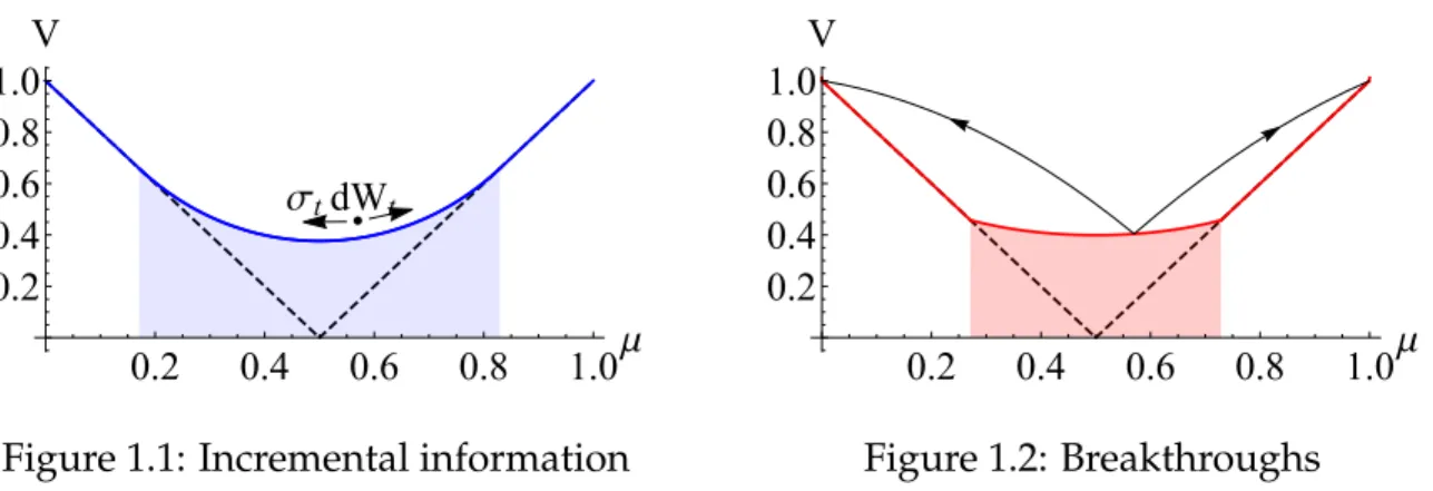
Example 1.1. Let the state be binaryX“ tl,ru. The prior belief of statex“risµ P p0, 1q. A “ tL,Ru. The DM wants to choose an action that matches the state:upL,lq “upR,rq “ 1; upL,rq “ upR,lq “ ´1. The discount rate ρ “ 1, H is the standard entropy function: Hpµq “ ´µlogpµq ´ p1´µqlogp1´µq, and the information costCpIq “ 12I2.
I consider three simple heuristic learning technologies: Gaussian learning, perfectly revealing breakthroughs and partially revealing evidence. A DM who uses a specific learning technology is modeled by restricting the admissible control set M to include only the corresponding family of processes. In each case, the DM controls a parameter that represents one aspect of learning.
1. Gaussian learning: The signal follows a Brownian motion whose drift is the true state, and whose variance is controlled by the DM. Therefore, the posterior belief follows a diffusion process (Bolton and Harris (1999.)), so the set of admissible controls are:
MD “ txµty|dµt “σtdWtu
The DM controls the signal precisionxσty. According to Ito’s lemma,It “ ´21σt2H2pµtq “
σ2
t
2µtp1´µtq. This problem is studied in Moscarini and Smith (2001.)
8
.
, where the value
tion is characterized by HJB: ρVDpµq “sup σą0 1 2σ 2V2 Dpµq ´ 1 2 ˆ σ2 2µp1´µq ˙2
The solutionVDpµqis plotted as the blue curve in Figure 1.1.. The shaded region is the
experimentation region and the non-shaded region is the stopping region.
σtdWt 0.2 0.4 0.6 0.8 1.0μ 0.2 0.4 0.6 0.8 1.0 V
Figure 1.1: Incremental information
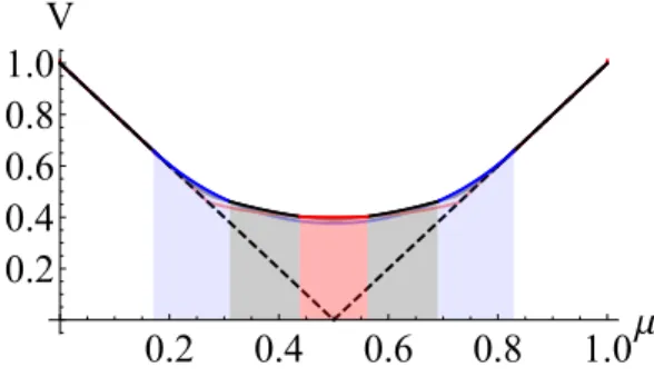
0.2 0.4 0.6 0.8 1.0μ 0.2 0.4 0.6 0.8 1.0 V Figure 1.2: Breakthroughs
2. Breakthroughs: The DM observes breakthroughs that perfectly reveal the true state with arrival rateλt. Then, belief follows a Poisson process that jumps to 1 if the state isrand
to 0 if the state isl. The set of admissible control is:
MB “
!
xµty|dµt “ p1´µtqdJ1tpλtµtq ` p0´µtqdJt0pλtp1´µtqq
)
xJtip¨qyare independent Poisson counting processes with Poisson ratep¨q. The DM con-trols the signal frequencyxλty. The Entropy reduction speed isλtHpµq. The HJB
equa-tion is as follows: ρVBpµq “sup λą0 λpµFp1q ` p1´µqFp0q ´VBpµqq ´1 2pλHpµqq 2
The solutionVBis plotted as the red curve in Figure 1.2.. The two arrows show the belief
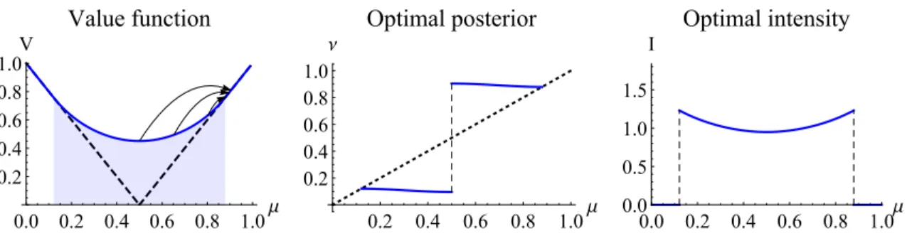
3. Partially revealing evidence: The DM allocates one unit of total attention to two news sources, each revealing one state with arrival rateγ“2. Then belief follows a compen-sated Poisson process, and the set of admissible belief processes is:
MP “ $ ’ & ’ % xµty ˇ ˇ ˇ ˇ dµt “p1´µtqpdJt1pαtγµtq ´αtγµtdtq `p0´µtqpdJt0pp1´αtqγp1´µtqq ´ p1´αtqγp1´µtqdtq , / . /
-xJtip¨qyare independent Poisson counting processes with Poisson ratep¨q. The DM con-trolsxαty, the attention allocated to the signal revealing stater. This control process is
identical to that in Che and Mierendorff (2016.). Applying their analysis, optimalαt is a
bang-bang solution, and the HJB equation is:
ρVPpµq“max!γµ` Fp1q´VPpµq´VP1pµqp1´µq˘´1 2 ` γµpHpµq`H1pµqp1´µqq˘2, γp1´µq`Fp0q´VPpµq´VP1pµqp0´µq ˘ ´1 2 ` γp1´µqpHpµq`H1pµqp0´µqq˘2 )
The solutionVPis plotted as the black curve in Figure 1.3.. The optimal strategy is
qual-itatively the same as in Che and Mierendorff (2016.). In the deep gray region, optimal
learning direction is confirmatory: the arrival of news reveals the a priori more likely state (represented by solid arrows). In the light gray region, optimal learning direction iscontradictory: the arrival of news reveals the a priori less likely state (dashed arrows).
0.2 0.4 0.6 0.8 1.0μ 0.2 0.4 0.6 0.8 1.0 V
Figure 1.3: Partially revealing evidence
0.2 0.4 0.6 0.8 1.0μ 0.2 0.4 0.6 0.8 1.0 V Figure 1.4: Comparison
In this example, the three learning technologies are analyzed for the same underlying decision problem and the same entropy cost function. Therefore, the utilities are directly comparable. I plot all three value functions in Figure 1.4.and use differently colored
re-gions to illustrate the order of utility. Each color corresponds to a learning strategy be-ing optimal: blue—Gaussian learnbe-ing, red—breakthroughs, and gray—confirmatory evi-dence.9. As shown in Figure 1.4., allowing the DM to use a rich set of strategies improves
the decision-making quality.
More interestingly, there appears to be a pattern when optimizing in different aspects. When the prior belief is highly uncertain, a fully revealing Poisson signal that can bring the DM directly to a conclusion is optimal. When the prior belief is quite uncertain but asymmetrically in favor of one state, allocating attention to the more promising direction becomes optimal. When the prior belief is very certain, an imprecise but frequent Gaus-sian signal becomes optimal. The formal analysis for fully flexible information acquisition in Section 1.6. illustrates that this pattern is systematic: the optimal direction, precision
and frequency of learning are exactly the relevant aspects and are closely related to the location of the prior belief.
1.3.1 Motivation for a flexible model
Example 1.1.implies that single-aspect models are insufficient for modeling a dynamic
information acquisition problem with a rich strategy set. For instance, the model consid-ering only partially revealing evidence predicts that seeking contradictory evidence is generally optimal when the belief is uncertain. However, further analysis shows that this prediction is misleading when Gaussian signals are also feasible. Studying a model where information acquisition is flexible inallaspects enables us to obtain insights about information acquisition without interference from any ad hoc restriction. Such insights
9In this example, whenever contradictory learning dominates confirmatory learning, contradictory
include which aspect(s) is(are) endogenously salient for information acquisition and how each of these aspects is determined by the DM’s incentives.
Although the results are derived in a fully flexible model, they apply to much more general settings where information acquisition isnot flexible in all aspects. First, all re-sults directly apply to all settings where information acquisition is flexible in those en-dogenously salient aspects, as all other aspects are redundant for implementing the un-constrained optimum. Second, even for settings where some of the relevant aspects are constrained, the intuitions from the flexible model identify the DM’s most important in-centive and how the hypothetically ideal strategy might be approximated by adjusting other aspects. In fact, the analysis of the flexible model in Sections 1.4.and 1.6.shows that
the set of endogenously salient aspects is quite small, and the optimal strategy satisfies very simple qualitative properties in these aspects. Therefore, the findings of this chapter are useful in a very wide range of settings.
1.4
Dynamic programming and HJB equation
Solving Equation (1.1). is not an easy task due to the abstract strategy space. To the
best of my knowledge, no general theory applicable to this stochastic control problem exists. The most closely related problems are studied in a set of remarkable papers on the martingale method in stochastic control (Davis (1979.),Boel and Kohlmann (1980.),Striebel
(1984.)). These papers introduce abstract formulations of stochastic control problems with
general (semi)martingale control processes. The problems have finite horizon and specific objective functions; hence, they do not nest Equation (1.1)..
Nevertheless, it is useful to introduce the general dynamic programming principle and HJB characterization. On the basis of the intuition of dynamic programming, the
conjecture thatVpµtqsatisfies the following HJB is reasonable: max␣ Fpµtq ´Vpµtq looooooomooooooon stopping value , ´ρVpµtq looomooon discount `sup dµt ␣ LtVpµtq looomooon continuation value ´Cp´LtHpµtqq looooooomooooooon control cost (( “0 (1.2)
HJB Equation (1.2).is conceptually the same as the standard HJB equation. Recall the
def-inition for operatorLt, LtVpµtqis the flow utility gain from continuing. The exact form
ofLtV and LtH depends on the probability space, the filtration and the control process
in the neighbourhood of t(which are summarized by the symbol dµt). Therefore,
Equa-tion (1.2).essentially states the dynamic programming principle: at any instance when the
control is chosen optimally, either stopping is optimal (the first term is 0) or continuing is optimal and the net continuation gain equals the loss from discounting (the second term is 0).
For a simple example, letM be a family of Markov jump-diffusion belief processes, characterized by the following SDE:
dµt “ pνpµtq ´µtqpdJtpppµtqq ´ppµtqdtq
looooooooooooooooooooomooooooooooooooooooooon
compensated Poisson part
` σpµtqdWt
loooomoooon
Gaussian diffusion
(1.3)
where pp,ν,σq : µt ÞÑ R`b∆pSupppµqq bR|Supppµq|´1 are control parameters, Jtp¨q is a
Poisson counting process with Poisson rate p¨q, and Wt is a standard one-dimensional
Wiener process. Note that this example also nests all three families of strategies in Ex-ample 1.1. as special cases
10
.
. Itô’s lemma implies an explicit form for the infinitesimal generator:
10The admissible control sets in the second and third cases in Example 1.1
. are not exactly nested in
Equation (1.3).. However, they can be viewed as mixed strategies of pure Poisson-jump processes defined
LVpµq “ ppVpνq ´Vpµq ´∇Vpµqpν´µqq
loooooooooooooooooooomoooooooooooooooooooon
flow value of Poisson jump & drift
` 1
2σ
THVpµqσ
loooooomoooooon
flow value of diffusion
where ∇and H are the gradient and Hessian operators, respectively. By replacing Lin Equation (1.2).with its explicit expression, we obtain a parametrized HJB Equation (1.4).:
ρVpµq“max " ρFpµq, sup p,ν,σ ppVpνq´Vpµq´∇Vpµqpν´µqq`1 2σ THVpµqσ (1.4) ´C ˆ ppHpµq´Hpνq`∇Hpµqpν´µqq´1 2σ THHpµqσ ˙*
On the other hand, when M is the jump-diffusion family, the jump-diffusion control theory (see textbooks, e.g., Hanson (2007.)) provides averification theoremthat proves that
the value function for Equation (1.1).is exactly characterized by HJB Equation (1.4)..
This simple example illustrates how a specific stochastic control problem relates to an HJB equation. Now, consider the general problem Equation (1.2).without any restriction
on the admissible belief process. First, we require a verification theorem stating that the HJB Equation (1.2).characterizes the solution of Equation (1.1).. Second, a representation
theorem for the abstract operator Lt is also necessary to make Equation (1.2). practically
tractable. The existing theories on martingale methods have little power for both tasks.11.
In Theorem 1.1., I achieve both goals by showing that the solution of Equation (1.1). is
characterized by a simple parametric HJB equation:
Theorem 1.1. Assume H is strictly concave and Cp2q smooth on interior beliefs in ∆pXq, As-sumptions 1.1.and 1.2.are satisfied. Let Vpµq P C
p1q∆pXqbe a solution12
.to HJB Equation(1.4).;
11First, the existing martingale methods verify the HJB equation for different sets of problems that do not
cover this specific problem. Moreover, the martingale method only states the existence of such LtV (for
example theorem 4.3.1 of Boel and Kohlmann (1980.)) and does not provide an explicit representation. This
issue is considered to be the main drawback of the martingale method (see discussions in Davis (1979.)).
12TheCp1qsolution to the second-order ODE is not well defined. To be precise,Vis a viscosity solution
(see Crandall, Ishii, and Lions (1992.)). In the viscosity solution,σ
then Vpµqsolves Equation(1.1)..
Theorem 1.1. first states that Vpµq is characterized by a HJB equation. More
surpris-ingly, Theorem 1.1.also states that the HJB is exactly Equation (1.4).. As a direct corollary,
Equation (1.1). can be solved by considering only the family of Markov jump-diffusion
processes characterized by SDE (1.3.). The compensated Poisson jump part and Gaussian
diffusion part in SDE (1.3.) each represents a simple learning strategy.
• Poisson learning: The DM usesPoisson learningor acquires aPoisson signalwhen a compensated Poisson part exists in the belief process. A Poisson jump in the belief process can be induced by observing non-conclusive news whose arrival follows a Poisson process. The compensating belief drift is induced by observing no news arriving. The control variables for Poisson learning arepp,νq, which represent three endogenously relevant aspects of Poisson learning. The arrival rate p represents the frequency of learning. The direction of belief jump represents the direction of learning. The magnitude of belief jump represents theprecisionof learning.
• Gaussian learning: The DM uses Gaussian learning or acquires a Gaussian signal when a diffusion part exists in the belief process. Gaussian diffusion in the be-lief process can be induced by observing the realization of a Gaussian process, with statexbeing the unobservable drift. The flow varianceσrepresents the signal pre-cision.
Equation (1.4).suggests that to determine the optimal strategy in all relevant aspects,
the DM considers four types of offs : (i) the standard continuing-stopping trade-off in optimal stopping problems, captured by the outer-layer maximization; (ii) the in-formation cost-utility gain trade-off, which determines the total cost spent on learning; whereD2Vpµ,σq “lim
δÑ02
Vpµ`δσq´Vpµq´∇Vpµqδσ δ∥σ∥2 .
(iii) the Poisson-Gaussian trade-off, which determines the proportion of cost allocated to the Poisson signal pp,νq and the Gaussian signal σ; (iv) the precision-frequency trade-off, which determines the marginal rate of substitution of signal frequency for precision. These trade-offs, especially the precision-frequency trade-off, will be discussed in detail to characterize the solution to Equation (1.4).in Section 1.6..
The proof of Theorem 1.1. uses an indirect method. I characterize Equation (1.1). as
the limit of a series of auxiliary discrete-time problems. The discrete-time analyses are presented in Section 1.5.. Readers interested in the solution of HJB Equation (1.4). can
jump to Section 1.6..
1.5
The auxiliary discrete-time problem
In this section, I introduce the steps for proving Theorem 1.1.using an auxiliary
discrete-time problem. First, in Section 1.5.1.I introduce a discrete-time stochastic control problem
that converges to the continuous-time problem. Then I characterize the Bellman equation for the discrete-time problem in Section 1.5.2.. In Section 1.5.3., I introduce a key lemma
that links all the discrete-time analyses and proves Theorem 1.1..
1.5.1 Discrete-time problem
I consider a stochastic control problem that is a discrete-time analog of Equation (1.1)..
Then I illustrate the discretization of the original problem. The discretization serves as a useful intermediary showing that the discrete-time problem converges to the continuous-time problem.
Decision problem: The primitives pA,X,u,µ,ρq are the same as those in Section 1.3..
Time is discrete t P N, and the period lengthdt ą 0. The payoff delayed by tperiods is discounted bye´ρdt¨t.
Information: The DM chooses the posterior belief process xµpty in a nonparametric
Cost of information: DefineCdtpIq fi C` I
dt
˘
dt. The per-period cost of information is assumed to beCdtpErHpµptq ´Hpµpt`1q|Fptsq. Note that this is exactly the finite-difference
analog of the flow costCp´LtHpµtqqin the continuous-time problem.
Optimization problem: The DM solves the following stochastic control problem:
Vdtpµq “ sup xµtpyPMx,pτ E « e´ρdt¨τpFp p µpτq ´ p τ´1 ÿ t“0 e´ρdt¨tCdt ´ E”Hpµptq ´Hpµpt`1q|Fpt ı¯ ff (1.5)
whereMxis the set of discrete-time martingales satisfyingµp0“µ, andτis axFpty´measurable
stopping time. Note that in this section, all discrete-time stochastic processes and random variables are labeled with “hat” to differentiate them from continuous-time processes.
The purpose of analyzing the discrete-time problem is to characterize the continuous-time value function Vpµq. Therefore, the first step is to show thatVdtpµq approximates Vpµq. To study the relation betweenVdtpµqand Vpµq, let us discretize the objective func-tion in Equafunc-tion (1.1).. For any admissible strategypxµty,τq, consider the Riemann sum:
Wdtpµt,τq “
8
ÿ
i“1
Probpτ P rpi´1qdt,idtsqE
„ e´iρdtFpµidtq ´ i´1 ÿ j“0 e´jρdtC` Ijdt˘ dt ȷ where Ijdt “ E”Hpµjdtq´Hpµpj`1qdtq dt ˇ ˇFjdt ı
. The objective function in Equation (1.1).is defined
in the notion of the Riemann-Stieltjes integral as limdtÑ0Wdtpµt,τq. I call the martingale
xµty integrable if the limit limdtÑ0Wdtpµt,τq exists.13. Unless otherwise stated, M is
re-stricted to contain integrable processes, an innocuous restriction that enables me to avoid technical discussions of integrability.14.Then it follows thatVpµq “ sup
xµtyPM,τlimdtÑ0Wdtpµt,τq.
13The standard definition for integrability also requires the limit to exist uniformly for all alternative
nonuniform discretizations of the time horizon and all alternative measurable stopping times. Here I use the weaker integrability requirement for notational simplicity. The optimal strategy actually satisfies the stronger integrability requirements, so the current definition can be used without loss. The discretization ofxItyis WLOG given the uniform convergence in the definition ofDpHq.
14The detailed discussion of why restricting belief to be integrable is innocuous is in Remark A.2
.
Now, consider the relation betweenWdt and Vdt. I argue that the objective function in Equation (1.5).is equivalent toWdtpµt,τq. This result can ben verified by noting that if
pxµty,τqandpxµpty,τpqjointly satisfyµpt “µt¨dtandτp“rτ{dts, then:
Wdtpµt,τq “ E « e´ρdtpτFp p µpτq ´ p τ´1 ÿ t“0 e´ρdt¨tCdt ´ E”Hpµptq ´Hpµpt`1q|Fpt ı¯ ff
Given feasible strategy pxµty,τq, such pxµpty,τpq can be constructed by simply
discretiz-ing the continuous-time strategy. Given feasible strategy pxµpty,τpq, such pxµty,τq can be
constructed by the Kolmogorov extension theorem. Therefore, it follows that Vdtpµq “ supxµtyPM,τWdtpµt,τq. Now that bothV and Vdt are characterized usingWdt,Wdt can be
used as an intermediary to linkV andVdt:
$ ’ ’ ’ & ’ ’ ’ % Vpµq “